Does EELS haunt your photoemission measurements?

Abstract

It has been argued in a recent paper by R. Joynt (R. Joynt, Science 284, 777 (1999)) that in the case of poorly conducting solids the photoemission spectrum close to the Fermi Energy may be strongly influenced by extrinsic loss processes similar to those occurring in High Resolution Electron Energy Loss Spectroscopy (HR-EELS), thereby obscuring information concerning the density of states or one electron Green’s function sought for. In this paper we present a number of arguments, both theoretical and experimental, that demonstrate that energy loss processes occurring once the electron is outside the solid, contribute only weakly to the spectrum and can in most cases be either neglected or treated as a weak structureless background.

]

I INTRODUCTION

Photoemission has been used for years as a reliable technique for probing the the electronic structure of the occupied states in solids ranging from insulators through semiconductors and metals to superconductors. In his article Joynt provided very convincing and interesting arguments that especially for badly conducting samples (roughly $\rho_{0}\geq 0.1m\Omega cm$, the Mott value) the photoelectron spectrum may be affected by energy loss structures resulting from the interaction with the time dependent fields set up by the photoelectron receding from the surface of the solid. He argued that the influence of these loss processes can be so strong that the spectrum is dominated by them and that therefore the intrinsic information regarding the electronic structure of the solid all but disappears. Since photoemission is playing such a prominent role in the discussion of strongly correlated materials like the High Tc’s, or more generally the transition metal oxides, as well as in Kondo and Heavy Fermion systems, it is of quite some importance to further investigate Joynt’s assertions. In this paper we study Joynt’s arguments and provide both experimental and theoretical findings that show that the effects due the losses discussed by Joynt are only a small contribution to the total spectrum and the zero energy loss probability for the photoelectrons dominates for samples of either good or bad conductivity.

II INTRINSIC AND PSEUDO-INTRINSIC EFFECTS

Compared to other techniques, photoemission provides the most easy and direct measurement of the one electron Green’s function and the directly related occupied density of states of a solid, if one keeps in mind the possible influence on the photoelectron of a number of ‘pseudo-intrinsic’ effects[2]. By this we mean first of all the matrix element needed for the description of the amplitude of the optical transition probability from an occupied state to a high energy unoccupied state in the solid, followed by energy loss processes occurring on the electron’s path to the surface and finally the description of the escape of the electron through the surface region into the vacuum. Where we emphasize that in the so called ‘sudden approximation’ we neglect all interactions and interference effects between the high energy excited electron and the hole left behind.
Also one has to contemplate the truly intrinsic effects: in a one electron approximation the associated one hole Green’s function is a delta peak at an energy determined by the band dispersion of the occupied states. In reality the electrons in the solid are usually not simple free electrons but they interact with other electrons, phonons, magnons etc., resulting in one electron Green’s functions now including a frequency and momentum dependent self-energy. For weakly interacting systems the initial delta function spectrum for such an electron broadens (asymmetrically) and attains a frequency distribution for each momentum vector, which basically provides information not only of the quasi-particle dispersion and lifetime, but also of the way the electron is dressed inside the solid, due to the response of its environment to its presence or absence. In strongly interacting systems this self-energy causes a rather large spreading out of the initial delta peaks describing the one hole Green’s function, and the description in terms of a quasi-particle with a certain lifetime may break down completely. In these cases it is indeed difficult to separate the intrinsic properties of the one hole Green’s function from the pseudo-intrinsic effects due to the energy losses suffered by the excited electron on its way out of the solid. These losses are basically dominated by the self-energy of the excited electron. It is extremely important therefore to have good estimates of the contributions due to energy loss processes to the spectrum so that these can be identified, and possibly corrected for, if they are substantial.

Experimentally there are several ways of checking the expected influence of these energy loss processes. The most obvious is to study the energy loss spectrum of electrons incident on the solid with an initial kinetic energy equal to that of the escaping photoelectron. These loss spectra provide one with direct information about the self-energy of an excited electron in the unoccupied states of the solid. For high energy electrons (E${}_{k}\geq$ 60 keV) a transmission EELS measurement is possible in which the obtained energy loss information is mostly due to bulk processes. However, to achieve high energy resolution, photoemission measurements are usually performed at low photon energies (E${}_{Ph}<100$ eV) such as HeI radiation (21.22 eV) or even less. At these low energies electron energy loss processes can be studied with reflection High Resolution EELS but one must then realize that the incident electron hardly penetrates the solid surface and that therefore the surface loss function is measured rather than the bulk losses experienced by a photoelectron originating from inside the solid as in photoemission. The surface and bulk loss function are linked to each other however and thus information about the intrinsic processes can be retrieved also from a reflection experiment, although the relative intensities of certain bulk losses compared to their surface analogs may differ. We note here that Joynt concentrates on losses occurring after the photoelectron has left the solid and so these should be directly related to the reflection ELS losses.

Another way of getting the self-energy information of the excited electron is to study the spectral function in a photoemission measurement of a narrow atomic core level of the solid at a photon energy such that the excited electron will have the required (low) kinetic energy. Although this loss spectrum will be intertwined with the satellite structure due to the self-energy effects involved in the sudden creation of the core hole itself, they will nonetheless provide us with an upper limit on the importance of the materials energy loss contributions to a photoemission spectrum. This was in fact suggested and used in Ref. [2] to argue that the broad and intense energy distribution seen in angular resolved photoelectron spectroscopy of the high Tc’s was not a result of energy loss processes but mainly a direct result of the strongly energy dependent self-energies in these strongly correlated materials. A more detailed study of this effect in the High Tc’s has recently been published[3].

Thus, in the interpretation of spectra, it is generally assumed that the photoelectron intensity distribution is a true reflection of the single particle spectral function, and that the aforementioned pseudo-intrinsic losses can be identified and reckoned with if necessary.

III EXTRINSIC EFFECTS

We now will focus on extrinsic broadening of photoemission structures such as the Fermi edge. Within photoemission this up to now meant just the finite instrumental resolution, but using the picture that Joynt put forward in his recent article, we now also have to consider losses suffered by the photoelectron after it has left the solid and is on its way to the detector. These losses are directly comparable to the loss spectrum of a reflection EELS measurement. Joynt argues that these losses more than anything will severely distort any sharp feature, such as the Fermi edge, especially in the case of badly conducting solids and anisotropic materials. He claims, depending on the properties of the material under study, that this extrinsic distortion can be so dramatic that instead of observing a sharp Fermi cutoff in the spectrum, the observed spectral distribution will look like that expected for a material with a so called pseudogap at E_F. If correct this would make photoemission unsuitable for the study of the one electron Green’s function of badly conducting solids such as many of the colossal magnetoresistance materials and the High Tc’s, among many others, are.
Joynt substantiates his statement by deriving an expression for the energy loss probability of an electron once the electron has emerged from the surface. He calculates, in a classical picture, the average energy lost due to the interaction of the electron’s time dependent electric field acting on the polarizable metal left behind. The response of the metal is approximated by a Drudelike behaviour. He then distributes this average energy lost over an energy loss spectrum using a probability distribution as a weighting function. The basic assumption is that the Born approximation is valid so that each electron suffers at most a single scattering event. This results in:

$$P(\omega)=\frac{2e^{2}CL(\omega)}{\pi\hbar v\omega^{2}}$$ (1)

in which $P(\omega)$ stands for the probability that the electron loses an energy $\omega$, $C$ is a constant for which Joynt gives a value of $\approx 2.57$, and $L(\omega)$ represents the loss function

$$L(\omega)=\frac{\omega}{4\pi}{\rm Im}\left(\frac{-1}{1+\epsilon(\omega)}\right).$$ (2)

We agree to a large extend with this derivation except perhaps for the constant C on which we will focus our attention later on in this paper. Let us for the moment assume that the Born approximation and Joynt’s derivation is correct. We see that the material related properties enter the equation for the energy loss distribution via the frequency dependent dielectric constant of the material. Which is not unexpected since this describes the response of the material to the time dependent field produced by the outgoing electron. Let us, as Joynt did, take as an example the dielectric function $\epsilon(\omega)$ given by the Drude model:

$$\epsilon(\omega)=\frac{4\pi i}{\omega}\sigma(\omega)=\frac{4\pi i\sigma_{0}}{\omega(1-i\omega\tau)}$$ (3)

and plot $P(\omega)$ for different values of the resistivity $\rho_{0}=1/\sigma_{0}$ and scattering time $\tau$ (Fig. 1) one sees immediately that although the weight of $P(\omega)$ is distributed differently in each curve, the integral $\int_{0}^{\infty}P(\omega)d\omega$ reaches the same value in the end. There is indeed a well known general sum rule[4] connected to this formula which is independent of material parameters:

$$\lim_{k\rightarrow 0}\frac{e^{2}C}{2\pi^{2}\hbar v}\int_{0}^{\infty}\frac{d\omega}{\omega}{\rm Im}\left(\frac{-1}{1+\epsilon(\omega)}\right)=\frac{e^{2}C}{2\pi^{2}\hbar v}\frac{\pi}{2}\frac{1}{1+\epsilon_{\infty}}$$ (4)

This is a general sum rule that holds for any model of $\epsilon(\omega)$ provided that it’s a causal function. It depends only on the velocity of the outgoing photoelectron which is presumed constant in the process, consistent with the Born approximation valid for weak scattering. So, for an electron with a kinetic energy of 20 eV, as used in Joynt’s examples, the integral from zero to infinity gives $\approx 0.0843$ for the total of the losses.
There is of course another sum rule which conserves the integrated intensity of the spectrum. In this sum rule we must include the finite probability $P_{0}$ that an electron suffers no loss at all, so that

$$1=P_{0}+\int_{0}^{\infty}P(\omega)d\omega.$$ (5)

Using the results above we find that $P_{0}\approx 0.957$, and therefore the normal single particle DOS will dominate the photoemission spectrum.
Up to now we’ve just been concentrating on the free electron part of the response function, of course there are more contributions (such as phonons, and interband transitions) that are contained in the total dielectric function of a real material. Therefore the calculations presented by us and by Joynt, using only the Drude model, will always overestimate the influence of the free electron contribution.
If we take a simple example to illustrate this: our first sum rule pins down the total amount of losses from zero to infinite frequency, this means that other processes such as phonons, not contained in the Drude model will just steal away some of the weight carried by the free electron losses that we have considered so far. This implies that in a good metal, where the phonon part will be nearly fully screened by the free electron excitations, the (low energy) loss spectrum is in first approximation indeed well described by the Drude model. If the material is then changed into a bad conductor the phonon part of the loss spectrum will gain more and more strength in the low energy region of the spectrum at the expense of the Drude part because of the sum rule. In both cases however, P₀ will have a fixed value. Furthermore, any phonon contribution will not influence the PES spectrum in a smooth way on the low energy scale around the Fermi energy, but rather produce a step in the convoluted photoemission-EELS spectrum, since these phonon losses are peaked at the phonon frequency, and are never overdamped. The same holds for a good metal where there is a clearly defined loss peak at the plasma frequency.
Thus, we can conclude that at 20 eV, $\int_{0}^{\infty}P(\omega)d\omega\approx 0.0843$ is an upper limit for the losses due to only the Drude part. This very general result is in direct conflict with the assumptions made by Joynt that $P_{0}$ could, within the approximations made by him, be very small, as he hints at the fact that processes other than the free electron losses will further reduce $P_{0}$, and therefore he takes $P_{0}$ to be a fit parameter. In our opinion it is not possible to make an independent choice for the value of $P_{0}$ as Joynt did since it is in essence determined by the sum rules and is independent of material constants.
From an experimental point of view, we know from reflection EELS experiments (see e.g., Fig. 4) at incoming energies of around 20 eV, that the elastic peak (which represents $P_{0}$) is by no means close to zero for any material. Only for very low incoming energies (below $\approx$ 10 eV) or when special surface waveguidelike conditions are met[5] can the zero loss peak be strongly suppressed. Besides this, in reflection EELS $P(\omega)$ is twice as strong as the loss probability in this photoemission scenario, since the electron can lose energy both on the incomming and on the outgoing trajectory. In fact, one can use the same method as that used in calculating the reflection EELS loss probability (see Ibach & Mills[6]) for this photoemission problem. It is interesting to note that one gets the same result except for a different numerical factor.[7]. This presumably stems from a difference in Fourier transform convention and in Mills’s case, avoiding integrals such as equation (1) in Joynt’s paper, which is not readily solvable analytically. Using the prefactor obtained by the procedure described by Mills the equation for the losses reads:

$$P(\omega)=\frac{e^{2}}{\hbar\omega v}{\rm Im}\left(\frac{-1}{1+\epsilon(\omega)}\right)$$ (6)

Which then for the sum rule means that the losses are in fact much more severe than with Joynt’s original prefactor: we now have $\int_{0}^{\infty}P(\omega)d\omega\approx 0.65$ again at a kinetic energy of the electron of 20 eV, leaving $P_{0}$ at 0.35. Even here, the zero loss part will still be large enough to dominate the Fermi cutoff, if one thinks in terms of the complete dielectric function being involved.
This result does imply however that working in the Born approximation is no longer valid, and a strong interaction picture containing also multiple losses needs to be applied, which is less straightforward to derive for a continuous spectrum of excitations. In the case of discrete, welldefined plasmon losses due to core level excitations, the loss spectrum has in fact been calculated by Langreth[8] with the result that multiple plasmon losses are seen distributing the energy loss over a wider energy range at the expense of the low energy losses. On the basis of this calculation we argue that multiple scattering corrections will not strongly influence the sum rules but instead they will just redistribute the losses over a wider energy range thereby reducing their influence in the low energy loss region.
If we for the moment stick to the single scattering scenario and take for the losses only the Drude contribution, we can calculate the photoemission spectrum for the same parameters as Joynt used, except now taking $P_{0}=0.35$. This is depicted in Fig. 2, the lower panel also contains the original calculation from Joynt, using $P_{0}=0.01$. From this we see, that although the lineshape of the photoemission spectrum is affected by the losses in the case of the bad metal (where the Drude contribution is overestimated!), there is still finite weight at the Fermi Energy and therefore the effect does not create a clear pseudogap structure.

IV EXPERIMENT

As a last discussion point, we will present the case of La_1.2Sr_1.8Mn₂O₇, a double layered colossal magnetoresistance oxide with a ferromagnetic metal (at low temperature) to paramagnetic insulator transition at 125 K grown by the traveling solvent floating zone method[9]. This material is a good candidate for testing Joynt’s assumption that materials with high resistivity will be more prone to the influence of losses on the Fermi region in photoemission spectra than those with low resistivity, as the resistivity changes by roughly two orders of magnitude from below to just above the phase transition (see Fig.3)[9]. We performed both reflection EELS at 20.5 eV incoming electron energy and angle integrated PES using a HeI source. For both measurements the sample was cleaved in situ at a temperature of 60K, and at a base pressure of $8\times 10^{-11}$ in the case of EELS and $4\times 10^{-11}$ in the case of PES. As these samples deteriorate even at these pressures in a matter of hours, we ensured that measurements were performed within 2 hours after the cleave, before the peak at 9 eV binding energy in the PES spectra started appearing, which is associated with a change in oxygen stoichiometry at the surface[11].
The satellite and background corrected regions around E_F of the photoemission spectra are shown in Fig. 5 for T=60K (solid), 140K (dashed) and T=180K (dotted). The inset depicts the full spectra, taken at 60K before and after the temperature cycle.
Since we performed EELS at a finite incoming angle with respect to the surface normal ($\theta_{in}=35\deg$) we have to apply a correction factor as described by Ibach and Mills[6] to extract the surface loss function ${\rm Im}\left(-1/1+\epsilon(\omega)\right)$, and then multiply this by $e^{2}/\hbar\omega v$ to get $P(\omega)$ as described in equation (6) in order to use it to simulate a PES spectrum. Therefore, in Fig. 4, top panel are depict the EELS spectra as taken at 50K (solid) and 150K (dashed) including the zero loss line, and in the lower panel $P(\omega)$ calculated from the data after subtraction of the zero loss line.

We then use this $P(\omega)$ to calculate its influence on a PES spectrum assuming a constant density of states, and using various values of $P_{0}$. This is depicted in the lower panel of Fig. 5. It can be seen from this figure, that unless $P_{0}=0$ the picture of Joynt doesn’t reproduce the photoemission spectrum at all. For any finite value of $P_{0}$ combined with a finite DOS at the Fermi energy, one will get a finite Fermi cutoff. To get a rough estimate of $P_{0}$ from experiment, we can integrate the zero loss peak separately and compare it to half the integral of the entire loss region up to 10 eV as measured in our EELS spectra, provided of course that we keep in mind that we used our detector in a mode which selects electrons within an opening angle of $2^{\circ}$ around the specular reflection and is therefore not fully angle integrated, which makes us underestimate the losses relative to the zero loss probability. However, if we proceed in this way, we get for both the 50 and 150K a ratio of $P_{0}:P(\omega)=0.82:0.18$ which shows at least that $P_{0}$ is not close to zero, and neither does $P_{0}$ in our experiments depend on temperature (or resistivity) of the sample. Our findings agree with ARPES measurements by Dessau and Saitoh et al.[10, 11] in which they use Joynt’s argument that he expects the loss effect to be angle independent to show that therefore the angle at which the smallest change is observed in going from above to below Tc is indicative of the maximum magnitude of the effect, and in their experiments turns out to be negligible.

V CONCLUSIONS

In conclusion, we have argued that Joynt indeed raises an important question regarding the influences of extrinsic losses on low energy photoelectrons, but we disagree with the statement that the losses will take the upper hand in determining the shape of the spectrum around the Fermi energy as there is a sum rule that renders the zero loss probability substantially finite. This at least holds down to photon energies such as the often used HeI line (21.22 eV), but may become a point of concern when really low photon energies are used. Of course, since the losses are by no means a small perturbation in this classical, single scattering approach a full quantum mechanical treatment including multiple scattering is called for. Furthermore, we are not able to reproduce Joynt’s formula exactly as far as the pre-factor is concerned, we believe however that the treatment by Mills [7] is self-consistent and avoids integrals with questionable convergence. We also have shown in the case of $La_{1.2}Sr_{1.8}Mn_{2}O_{7}$ that we cannot reproduce the photoemission spectrum using a finite density of states up to the Fermi energy together with a finite value for $P_{0}$, so that we must conclude that there is a true pseudogap in this material both below and above the phase transition.

ACKNOWLEDGEMENTS

We would like to thank D. L. Mills for letting us use his calculation of $P(\omega)$ for our simulations, and M. Mostovoy and L. H. Tjeng for their valuable contributions along the way. This research was supported by the Netherlands Foundation for Fundamental Research on Matter (FOM) with financial support from the Netherlands Organization for the Advancement of Pure Research (NWO). The research of MAJ was supported through a grant from the Oxsen Network.

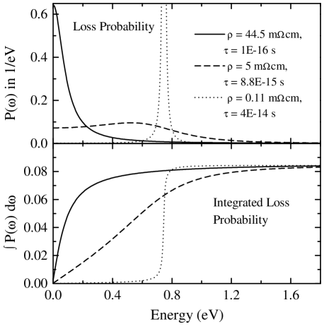
FIG. 1.: Top panel: The loss probability P($\omega$) calculated for different values of resistivity $\rho$ and relaxation time $\tau$, keeping the surface plasmon energy $\omega_{SP}^{2}=4\pi/(\rho\tau(1+\epsilon_{\infty}))$ fixed at 0.75 eV. Lower panel: Demonstration of the sumrule for the loss probability P($\omega$).

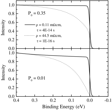
FIG. 2.: Comparison between Joynt’s original calculation with $P_{0}=0.01$ and $\int P(\omega)d\omega=0.0843$ (lower panel) and our calculation using Mills’ prefactor for the loss probability P($\omega$) and obeying the sum rule $P_{0}=1-\int P(\omega)d\omega=0.35$ (top panel) The parameters are specified in the figure and T = 38K. Although the shape of the spectrum is affected, there is no clear sign of a pseudogap for the bad metal in our case.

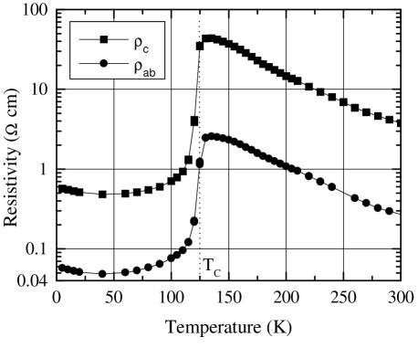
FIG. 3.: The resistivity of our $La_{1.2}Sr_{1.8}Mn_{2}O_{7}$ samples in the ab plane (circles) and the c direction (squares) as a function of temperature (from Ref. 9).

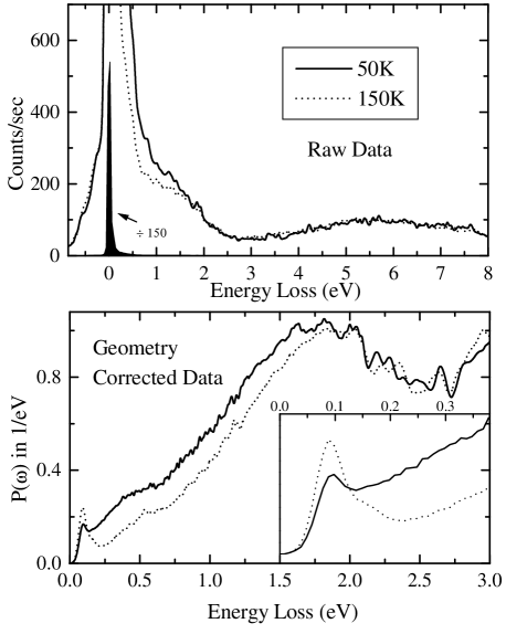
FIG. 4.: Top panel: Reflection EELS spectra, as taken, of $La_{1.2}Sr_{1.8}Mn_{2}O_{7}$, at 50K (solid) and 150K (dotted). Incoming/outgoing angle is $35^{\circ}$ with respect to the surface normal. Incoming electron energy is 20.5 eV. Zero Loss FWHM $=60$ meV. The filled black curve is the 50K spectrum divided by 150 to show the relative weakness of the loss features with respect to the zero loss electrons. Lower panel: Geometry corrected spectra, according to Ref. 6 multiplied by $e^{2}/\hbar\omega v$ to get P($\omega$). Inset: first 400 meV, showing the stronger presence of a surface phonon in the insulating regime, relative to the metallic phase.

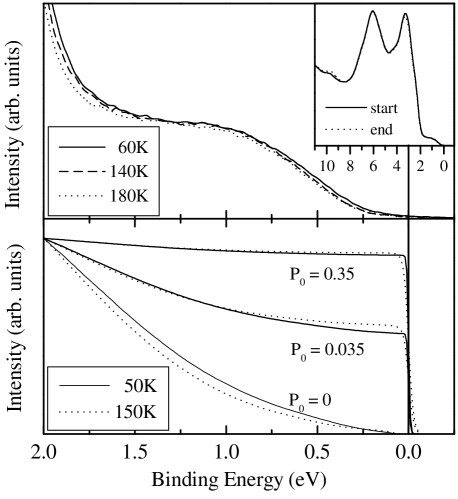
FIG. 5.: Top panel: PES spectra at different temperatures above and below the phase transition in $La_{1.2}Sr_{1.8}Mn_{2}O_{7}$ close to the ‘Fermi energy’, the inset shows the spectra up to 12 eV binding energy, before and after the temperature cycle ensuring the sample has not degraded in the mean time. Lower panel: Calculated PES spectra using the loss probability P($\omega$) constructed from the EELS data of Fig. 4 and assuming a constant DOS, for various values of the zero loss probability P₀ as indicated in the figure.

REFERENCES

- [1] R. Joynt, Science 284, 777 (1999).
- [2] G. A. Sawatzky in Proceedings of High Tc Superconductivity Symposium, Los Alamos, 1989, edited by K. S. Bedell, D. Coffey, D. E. Meltzer, D. Pines and J. R. Schrieffer (Addison-Wesley, Reading, 1990), p297.
- [3] M. R. Norman, M. Randeria, B. Janko and J. C. Campuzano, Phys. Rev. B 61, 14742, (2000).
- [4] G. D. Mahan, Many Particle Physics (Plenum, New York, 1990), p467.
- [5] J. J. M. Pothuizen, Ph.D. Thesis, Rijksuniversitteit Groningen, 1998.
- [6] H. Ibach, D. L. Mills, Electron energy loss spectroscopy and surface vibrations (Academic, New York, 1982), Chap. 3.
- [7] D. L. Mills, Phys. Rev. B 62, 11197, (2000). Although Mills arrives at a different conclusion than we present in this paper, we do use his calculation of , resulting in a different prefactor compared to Joynt.
- [8] D. C. Langreth, Phys. Rev. Lett. 26 1229, (1971).
- [9] W. Prellier et al., Physica B 259-261, 833, (1999).
- [10] D. S. Dessau and T. Saitoh, Science 287, 767a, (2000) technical comment and R. Joynt, response.
- [11] T. Saitoh et al., Phys. Rev. B 62, 1039, (2000).