Noise of a Quantum-Dot System in the Cotunneling Regime

Abstract

We study the noise of the cotunneling current through one or several tunnel-coupled quantum dots in the Coulomb blockade regime. The various regimes of weak and strong, elastic and inelastic cotunneling are analyzed for quantum-dot systems (QDS) with few-level, nearly-degenerate, and continuous electronic spectra. We find that in contrast to sequential tunneling where the noise is either Poissonian (due to uncorrelated tunneling events) or sub-Poissonian (suppressed by charge conservation on the QDS), the noise in inelastic cotunneling can be super-Poissonian due to switching between QDS states carrying currents of different strengths. In the case of weak cotunneling we prove a non-equilibrium fluctuation-dissipation theorem which leads to a universal expression for the noise-to-current ratio (Fano factor). In order to investigate strong cotunneling we develop a microscopic theory of cotunneling based on the density-operator formalism and using the projection operator technique. The master equation for the QDS and the expressions for current and noise in cotunneling in terms of the stationary state of the QDS are derived and applied to QDS with a nearly degenerate and continuous spectrum.

]

I Introduction

In recent years, there has been great interest in transport properties of strongly interacting mesoscopic systems.[1] As a rule, the electron interaction effects become stronger with the reduction of the system size, since the interacting electrons have a smaller chance to avoid each other. Thus it is not surprising that an ultrasmall quantum dot connected to leads in the transport regime, being under additional control by metallic gates, provides a unique possibility to study strong correlation effects both in the leads and in the dot itself.[2] This has led to a large number of publications on quantum dots, which investigate situations where the current acts as a probe of correlation effects. Historically, the nonequilibrium current fluctuations (shot noise) were initially considered as a serious problem for device applications of quantum dots [3, 4, 5] rather than as a fundamental physical phenomenon. Later it became clear that shot noise is an interesting phenomenon in itself,[6] because it contains additional information about correlations, which is not contained, e.g., in the linear response conductance and can be used as a further approach to study transport in quantum dots, both theoretically [4, 5, 7, 8, 9, 10, 11, 12, 13, 14, 15, 16, 17, 18, 19, 20, 21, 22] and experimentally.[23]

Similarly, the majority of papers on the noise of quantum dots consider the sequential (single-electron) tunneling regime, where a classical description (the so-called “orthodox” theory) is applicable.[24] We are not aware of any discussion in the literature of the shot noise induced by a cotunneling (two-electron, or second-order) current,[25, 26] except Ref. [21], where the particular case of weak cotunneling (see below) through a double-dot (DD) system is considered. Again, this might be because until very recently cotunneling has been regarded as a minor contribution to the sequential tunneling current, which spoils the precision of single-electron devices due to leakage.[27] However, it is now well understood that cotunneling is interesting in itself, since it is responsible for strongly correlated effects such as the Kondo effect in quantum dots,[28, 29] or can be used as a probe of two-electron entanglement and nonlocality,[21] etc.

In this paper we present a thorough analysis of the shot noise in the cotunneling regime. Since the single-electron “orthodox” theory cannot be applied to this case, we first develop a microscopic theory of cotunneling suitable for the calculation of the shot noise in Secs. III and IV. [For an earlier microscopic theory of transport through quantum dots see Refs. [30, 31, 32].] We consider the transport through a quantum-dot system (QDS) in the Coulomb blockade (CB) regime, in which the quantization of charge on the QDS leads to a suppression of the sequential tunneling current except under certain resonant conditions. We consider the transport away from these resonances and study the next-order contribution to the current, the so-called cotunneling current.[25, 26] In general, the QDS can contain several dots, which can be coupled by tunnel junctions, the double dot (DD) being a particular example.[21] The QDS is assumed to be weakly coupled to external metallic leads which are kept at equilibrium with their associated reservoirs at the chemical potentials $\mu_{l}$, $l=1,2$, where the currents $I_{l}$ can be measured and the average current $I$ through the QDS is defined by Eq. (7).

Before proceeding with our analysis we briefly review the results available in the literature on noise of sequential tunneling. For doing this, we introduce right from the beginning all relevant physical parameters, namely the bath temperature $T$, bias $\Delta\mu=\mu_{1}-\mu_{2}$, charging energy $E_{C}$, average level spacing $\delta E$, and the level width $\Gamma=\Gamma_{1}+\Gamma_{2}$ of the QDS, where the tunneling rates $\Gamma_{l}=\pi\nu|T_{l}|^{2}$ to the leads $l=1,2$ are expressed in terms of tunneling amplitudes $T_{l}$ and the density of states $\nu$ evaluated at the Fermi energy of the leads. In Fig. 1 the most important parameters are shown schematically. This variety of parameters shows that many different regimes of the CB are possible. In the linear response regime, $\Delta\mu\ll k_{B}T$, the thermal noise [33] is given by the equilibrium fluctuation-dissipation theorem (FDT).[34] Although the cross-over from the thermal to nonequilibrium noise is of our interest (see Sec. III), in this section we discuss the shot noise alone and set $T=0$. Then the noise at zero frequency $\omega=0$, when $\delta I_{2}=-\delta I_{1}$, can be characterized by one single parameter, the dimensionless Fano factor $F=S(0)/e|I|$, where the spectral density of the noise $S(0)\equiv S_{22}(0)$ is defined by Eq. (7). The Fano factor acquires the value $F=1$ for uncorrelated Poissonian noise.

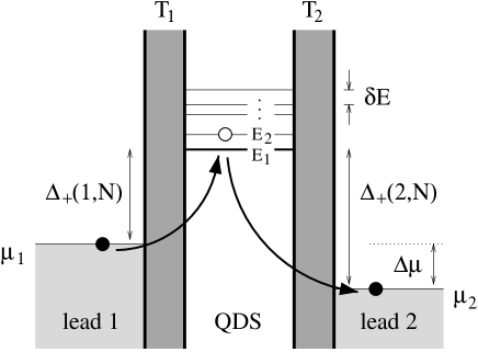
FIG. 1.: Schematic representation of the quantum dot system (QDS) coupled to two external leads $1$ and $2$ (light grey) via tunneling barriers (dark grey), where the energy scale is drawn vertically. The tunneling between the QDS and the leads $l=1,2$ is parametrized by the tunneling amplitudes $T_{l}$, where the lead and QDS quantum numbers $k$ and $p$ have been dropped for simplicity, see Eq. (3). The leads are at the chemical potentials $\mu_{1,2}$, with an applied bias $\Delta\mu=\mu_{1}-\mu_{2}$. The (many-particle) eigenstates of the QDS with one added electron ($N+1$ electrons in total) are indicated by their energies $E_{1}$, $E_{2}$, etc., with average level-spacing $\delta E$. The energy cost for adding a particle from the Fermi level of lead $l$ to the N-electron QDS is denoted by $\Delta_{+}(l,N)>0$ and is strictly positive in the CB regime. Note that the energies $\Delta_{-}(l,N)$ for removing particles from the QDS containing $N$ electrons are positive as well, and are not drawn here. The cotunneling process is visualized by two arrows, leading from the initial state in, say, lead 1 (full circle), via a virtual state on the QDS (open circle), to the final state in lead 2 (full circle).

Next we discuss the different CB regimes. (1) In the limit of large bias $\Delta\mu\gg E_{C}$, when the CB is suppressed, the QDS can be viewed as being composed of two tunnel junctions in series, with the total conductance $G=G_{1}G_{2}/(G_{1}+G_{2})$, where $G_{l}=\pi e^{2}\nu\nu_{D}|T_{l}|^{2}$ is the conductance of the tunnel junctions to lead $l$, and $\nu_{D}$ is the density of dot states. Then the Fano factor is given by $F=(G_{1}^{2}+G_{2}^{2})/(G_{1}+G_{2})^{2}$, as it has been found in Refs. [4, 5, 7]. Thus, the shot noise is suppressed, $F<1$, and reaches its minimum value for the symmetric QDS, $G_{1}=G_{2}$, where $F=1/2$. (2) The low bias regime, $\delta E\ll\Delta\mu\ll E_{C}$. The first inequality $\delta E\ll\Delta\mu$ allows to assume a continuous spectrum on of the QDS and guarantees that the single-electron “orthodox” theory based on a classical master equation can be applied. The second inequality $\Delta\mu\ll E_{C}$ means that the QDS is in the CB regime, where the energy cost $\Delta_{\pm}(l,N)=E(N\pm 1)-E(N)\mp\mu_{l}$ for the electron tunneling from the Fermi level of the lead $l$ to the QDS ($+$) and vice versa ($-$) oscillates as a function of gate voltage between its minimum value $\Delta_{\pm}<0$ (where the energy deficit turns into a gain, $|\Delta_{\pm}|\sim\Delta\mu$) and its maximum value $\Delta_{\pm}\sim E_{C}$. Here, $E(N)$ denotes the ground-state energy of the $N$-electron QDS. Thus the current $I$ as a function of the gate voltage consists of the CB peaks which are at the degeneracy points $\Delta_{\pm}<0$, where the number of electrons on the QDS fluctuates between $N$ and $N+1$ due to single-electron tunneling. The peaks are separated by plateaus, where the single-electron tunneling is blocked because of the finite energy cost $\Delta_{\pm}>0$ and thus the sequential tunneling current vanishes. At the peaks the current is given by $I=e\gamma_{1}\gamma_{2}/(\gamma_{1}+\gamma_{2})$, while the Fano factor has been reported [5, 7, 8, 9, 10] to be equal to $F=(\gamma_{1}^{2}+\gamma_{2}^{2})/(\gamma_{1}+\gamma_{2})^{2}$, $1/2<F<1$, where $\gamma_{1}=e^{-2}G_{1}|\Delta_{+}(1,N)|$ and $\gamma_{2}=e^{-2}G_{2}|\Delta_{-}(2,N+1)|$ are the tunneling rates to the QDS from lead 1 and from the QDS to lead 2, respectively. Within the “orthodox” theory tunneling is still possible between the peaks at finite temperature due to thermal activation processes, and then the Fano factor approaches the Poissonian value $F=1$ from below. (3) Finally, the limit $\Gamma\ll\Delta\mu\ll\delta E$ is similar to the previous case, with the only difference that the dot spectrum is discrete. The sequential tunneling picture can still be applied; the result for the Fano factor at the current peak is $F=(\Gamma_{1}^{2}+\Gamma_{2}^{2})/(\Gamma_{1}+\Gamma_{2})^{2}$, so that again $1/2<F<1$.[16]

We would like to emphasize the striking similarity of the Fano factors in all three regimes, where they also resemble the Fano factor of the noninteracting double-barrier system.[6] The Fano factors in the first and second regimes become even equal if the ground-state level of the QDS lies exactly in the middle between the Fermi levels of lead 1 and 2, $|\Delta_{+}|=|\Delta_{-}|$. We believe that this “ubiquitous” [7] double-barrier character of the Fano factor can be interpreted as being the result of the natural correlations imposed by charge conservation rather than by interaction effects. Indeed, in the transport through a double-barrier tunnel junction each barrier can be thought of as an independent source of Poissonian noise. And although in the second regime the CB is explicitly taken into account, the stronger requirement of charge conservation at zero frequency, $\delta I_{1}+\delta I_{2}=0$, has to be satisfied, which leads to additional correlations between the two sources of noise and to a suppression of the noise below the Poissonian value. At finite frequency (but still in the classical range defined as $\omega\ll\Delta\mu,E_{C}$) temporary charge accumulation on the QDS is allowed, and for frequencies larger than the tunneling rate, $\omega\gg\gamma_{1,2}$, the conservation of charge does not need to be satisfied, while the noise power $S_{22}$ approaches its Poissonian value from below, and the cross correlations vanish, $S_{12}=0$. [35] Based on this observation we expect that the direct measurement of interaction effects in noise is only possible either in the quantum (coherent) CB regime [16] $\Delta\mu\sim\Gamma$ or in the Kondo regime,[17, 18, 19] where both charge conservation and many-electron effects lead to a suppression of the noise. Another example is the noise in the quantum regime, $\Delta\mu\leq\omega\sim E_{C}$, where it contains singularities associated with the “photo-assisted transitions” above the Coulomb gap $\Delta_{\pm}$. [20, 21, 36]

To conclude our brief review we would like to emphasize again that while the zero-frequency shot noise in the sequential tunneling regime is always suppressed below its full Poissonian value as a result of charge conservation (interactions suppressing it further), we find that, in the present work the shot noise in the cotunneling regime[37] is either Poissonian $F=1$ (elastic or weak inelastic cotunneling) or, rather surprisingly, non-Poissonian $F\neq 1$ (strong inelastic cotunneling). Therefore the non-Poissonian noise in QDS can be considered as being a fingerprint of inelastic cotunneling. This difference of course stems from the different physical origin of the noise in the cotunneling regime, which we discuss next. Away from the sequential tunneling peaks, $\Delta_{\pm}>0$, single-electron tunneling is blocked, and the only elementary tunneling process which is compatible with energy conservation is the simultaneous tunneling of two electrons called cotunneling[25, 26]. In this process one electron tunnels, say, from lead $1$ into the QDS, and the other electron tunnels from the QDS into lead $2$ with a time delay on the order of $\Delta_{\pm}^{-1}$ (see Ref. [21]). This means that in the range of frequencies, $\omega\ll\Delta_{\pm}$, (which we assume in our paper) the charge on the QDS does not fluctuate, and thus in contrast to the sequential tunneling the correlation imposed by charge conservation is not relevant for cotunneling. Furthermore, in the case of elastic cotunneling ($\Delta\mu<\delta E$), where the state of the QDS remains unchanged, the QDS can be effectively regarded as a single barrier. Therefore, subsequent elastic cotunneling events are uncorrelated, and the noise is Poissonian with $F=1$. On the other hand, this is not so for inelastic cotunneling($\Delta\mu>\delta E$), where the internal state of the QDS is changed, thereby changing the conditions for the subsequent cotunneling event. Thus, in this case the QDS switches between different current states, and this creates a correction to noise $\Delta S$, so that the total noise is non-Poissonian, and can become super-Poissonian. The other mechanism underlying super-Poissonian noise is the excitation of high energy levels (heating) of the QDS caused by multiple inelastic cotunneling transitions and leading to the additional noise $\Delta S_{h}$. Thus the total noise can be written as $S=eI+\Delta S_{h}+\Delta S$. For other cases exhibiting super-Poissonian noise (in the strongly non-linear bias regime) see Ref. [6].

According to this picture we consider the following different regimes of the inelastic cotunneling. We first discuss the weak cotunneling regime $w\ll w_{\rm in}$, where $w\sim\Gamma_{1}\Gamma_{2}\Delta\mu/\Delta_{\pm}^{2}$ is the average rate of the inelastic cotunneling transitions on the QDS [see Eqs. (58-62)], and $w_{\rm in}$ is the intrinsic relaxation rate of the QDS to its equilibrium state due to the coupling to the environment. In this regime the cotunneling happens so rarely that the QDS always relaxes to its equilibrium state before the next electron passes through it. Thus we expect no correlations between cotunneling events in this regime, and the zero-frequency noise is going to take on its Poissonian value with Fano factor $F=1$, as first obtained for a special case in Ref. [21]. This result is generalized in Sec. III, where we find a universal relation between noise and current of single-barrier tunnel junctions and, more generally, of the QDS in the first nonvanishing order in the tunneling perturbation $V$. Because of the universal character of the results Eqs. (19) and (34) we call them the nonequilibrium FDT in analogy with linear response theory.

Next, we consider strong cotunneling, i.e. $w\gg w_{\rm in}$. The microscopic theory of the transport and noise in this regime based on a projector operator technique is developed in Sec. IV. In the case of a few-level QDS, $\delta E\sim E_{C}$, [38] noise turns out to be non-Poissonian, as we have discussed above, and this effect can be estimated as follows. The QDS is switching between states with the different currents $I\sim ew$, and we find $\delta I\sim ew$. The QDS stays in each state for the time $\tau\sim w^{-1}$. Therefore, for the positive correction to the noise power we get $\Delta S\sim\delta I^{2}\tau\sim e^{2}w$, and the estimate for the correction to the Fano factor follows as $\Delta S/eI\sim 1$. A similar result is expected for the noise induced by heating, $\Delta S_{h}$, which can roughly be estimated by assuming an equilibrium distribution on the QDS with the temperature $k_{B}T\sim\Delta\mu$ and considering the additional noise as being thermal,[33] $\Delta S_{h}\sim Gk_{B}T\sim(eI/\Delta\mu)k_{B}T\sim eI$. The characteristic frequency of the noise correction $\Delta S$ is $\omega\sim w$, with $\Delta S$ vanishing for $\omega\gg w$ (but still in the classical range, $\omega\ll\Delta\mu$). In contrast to this, the additional noise due to heating, $\Delta S_{h}$, does not depend on the frequency.

In Sec. V we consider the particular case of nearly degenerate dot states, in which only few levels with an energy distance smaller than $\delta E$ participate in transport, and thus heating on the QDS can be neglected. Specifically, for a two-level QDS we predict giant (divergent) super-Poissonian noise if the off-diagonal transition rates vanish. The QDS goes into an unstable mode where it switches between states 1 and 2 with (generally) different currents. We consider the transport through a double-dot (DD) system as an example to illustrate this effect [see Eq. (112) and Fig. 3].

Finally, we discuss the case of a multi-level QDS, $\delta E\ll E_{C}$. In this case the correlations in the cotunneling current described above do not play an essential role. In the regime of low bias, $\Delta\mu\ll(\delta E\,E_{C})^{1/2}$, elastic cotunneling dominates transport,[25, 39] and thus the noise is Poissonian. In the opposite case of large bias, $\Delta_{\pm}\gg\Delta\mu\gg(\delta E\,E_{C})^{1/2}$, the transport is governed by inelastic cotunneling, and in Sec. VI we study heating effects which are relevant in this regime. For this we use the results of Sec. IV and derive a kinetic equation for the distribution function $f(\varepsilon)$. We find three universal regimes where $I\sim\Delta\mu^{3}$, and the Fano factor does not depend on bias the $\Delta\mu$. The first is the regime of weak cotunneling, $\tau_{\rm in}\ll\tau_{c}$, where $\tau_{\rm in}$ and $\tau_{c}$ are time scales characterizing the single-particle dynamics of the QDS. The energy relaxation time $\tau_{\rm in}$ describes the strength of the coupling to the environment while $\tau_{c}\sim e\nu_{D}\Delta\mu/I$ is the cotunneling transition time. Then we obtain for the distribution $f(\varepsilon)=\theta(-\varepsilon)$, reproducing the result of Ref. [25]. We also find that $F=1$, in agreement with the FDT proven in Sec. III. The other two regimes of strong cotunneling $\tau_{\rm in}\gg\tau_{c}$ are determined by the electron-electron scattering time $\tau_{ee}$. For the cold-electron regime, $\tau_{c}\ll\tau_{ee}$, we find the distribution function by solving the integral equations (125) and (126), while for hot electrons, $\tau_{c}\gg\tau_{ee}$, $f$ is given by the Fermi distribution function with an electron temperature obtained from the energy balance equation (130). We use $f(\varepsilon)$ to calculate the Fano factor, which turns out to be very close to 1. On the other hand, the current depends not only on $G_{1}G_{2}$ but also on the ratio, $G_{1}/G_{2}$, depending on the cotunneling regime [see Fig. 4]. Details of the calculations are deferred to four appendices.

II Model system

The quantum-dot system (QDS) under study is weakly coupled to two external metallic leads which are kept in equilibrium with their associated reservoirs at the chemical potentials $\mu_{l}$, $l=1,2$, where the currents $I_{l}$ can be measured. Using a standard tunneling Hamiltonian approach,[40] we write

$$H=H_{0}+V\,,\quad H_{0}=H_{L}+H_{S}+H_{\rm int}\,,$$ (1)

$$H_{L}=\sum_{l=1,2}\sum_{k}\varepsilon_{k}c_{lk}^{{\dagger}}c_{lk}\,,\quad H_{S}=\sum_{p}\varepsilon_{p}d_{p}^{{\dagger}}d_{p}\,,$$ (2)

$$V=\sum_{l=1,2}(D_{l}+D^{{\dagger}}_{l}),\quad D_{l}=\sum_{k,p}T_{lkp}c_{lk}^{{\dagger}}d_{p}\,,$$ (3)

where the terms $H_{L}$ and $H_{S}$ describe the leads and QDS, respectively (with $k$ and $p$ from a complete set of quantum numbers), and tunneling between leads and QDS is described by the perturbation $V$. The interaction term $H_{\rm int}$ is specified below. The $N$-electron QDS is in the cotunneling regime where there is a finite energy cost $\Delta_{\pm}(l,N)>0$ for the electron tunneling from the Fermi level of the lead $l$ to the QDS ($+$) and vice versa ($-$), so that only processes of second order in $V$ are allowed.

To describe the transport through the QDS we apply standard methods[40] and adiabatically switch on the perturbation $V$ in the distant past, $t=t_{0}\to-\infty$. The perturbed state of the system is described by the time-dependent density matrix $\rho(t)=e^{-iH(t-t_{0})}\rho_{0}e^{iH(t-t_{0})}$, which can be written as

$$\rho(t)=e^{-iL(t-t_{0})}\rho_{0}\,,\quad LA\equiv\left[H,A\right]\,,\quad\forall A\,,$$ (4)

with the help of the Liouville operator $L=L_{0}+L_{V}$.[41] Here $\rho_{0}$ is the grand canonical density matrix of the unperturbed system,

$$\rho_{0}=Z^{-1}e^{-K/k_{B}T},$$ (5)

where we set $K=H_{0}-\sum_{l}\mu_{l}N_{l}$.

Because of tunneling the total number of electrons in each lead $N_{l}=\sum_{k}c_{lk}^{{\dagger}}c_{lk}$ is no longer conserved. For the outgoing currents $\hat{I}_{l}=e\dot{N}_{l}$ we have

$$\hat{I}_{l}=ei\left[V,N_{l}\right]=ei(D^{{\dagger}}_{l}-D_{l})\,.$$ (6)

The observables of interest are the average current $I\equiv I_{2}=-I_{1}$ through the QDS, and the spectral density of the noise $S_{ll^{\prime}}(\omega)=\int dtS_{ll^{\prime}}(t)\exp(i\omega t)$,

$$I_{l}={\rm Tr}\rho(0)\hat{I}_{l},\quad S_{ll^{\prime}}(t)={\rm Re}\,{\rm Tr}\,\rho(0)\delta I_{l}(t)\delta I_{l^{\prime}}(0)\,,$$ (7)

where $\delta I_{l}=\hat{I}_{l}-I_{l}$. Below we will use the interaction representation where Eq. (7) can be rewritten by replacing $\rho(0)\to\rho_{0}$ and $\hat{I}_{l}(t)\to U^{{\dagger}}(t)\hat{I}_{l}(t)U(t)$, with

$$U(t)=T\exp\left[-i\int^{t}_{-\infty}dt^{\prime}\,V(t^{\prime})\right]\,.$$ (8)

In this representation, the time dependence of all operators is governed by the unperturbed Hamiltonian $H_{0}$.

III Non-equilibrium fluctuation-dissipation theorem for tunnel junctions

In this section we prove the universality of noise of tunnel junctions in the weak cotunneling regime $w\ll w_{\rm in}$ keeping the first nonvanishing order in the tunneling Hamiltonian $V$. Since our final results Eqs. (19), (21), (23), and (34) can be applied to quite general systems out-of-equilibrium we call this result the non-equilibrium fluctuation-dissipation theorem (FDT). In particular, the geometry of the QDS and the interaction $H_{\rm int}$ are completely arbitrary for the discussion of the non-equilibrium FDT in this section. Such a non-equilibrium FDT was derived for single barrier junctions long ago.[42] We will need to briefly review this case which allows us then to generalize the FDT to QDS considered here in the most direct way.

A Single-barrier junction

The total Hamiltonian of the junction [given by Eqs. (1)-(3)] and the currents Eq. (6) have to be replaced by $H=H_{L}+H_{\rm int}+V$, where

$$V=A+A^{{\dagger}}\,,\quad A=\sum_{k,k^{\prime}}T_{kk^{\prime}}c_{2k}^{{\dagger}}c_{1k^{\prime}}\,,$$ (9)

$$\hat{I}_{2}=-\hat{I}_{1}=ei\left[V,N_{2}\right]=ei\left(A^{{\dagger}}-A\right)\,.$$ (10)

For the sake of generality, we do not specify the interaction $H_{\rm int}$ in this section, nor the electron spectrum in the leads, and the geometry of our system.

Applying the standard interaction representation technique,[40] we expand the expression (8) for $U(t)$ and keep only first non-vanishing contributions in $V$, obtaining

$$I(t)=i\int\limits^{t}_{-\infty}dt^{\prime}\langle\left[V(t^{\prime}),\hat{I}_{2}(t)\right]\rangle\,,$$ (11)

where we use the notation $\langle\ldots\rangle={\rm Tr}\rho_{0}(\ldots)$. Analogously, we find that the first non-vanishing contribution to the noise power $S(\omega)\equiv S_{22}(\omega)$ is given by

$$S(\omega)=\frac{1}{2}\int\limits^{\infty}_{-\infty}dt\,e^{i\omega t}\langle\{\hat{I}_{2}(t),\hat{I}_{2}(0)\}\rangle\,,$$ (12)

where $\{\ldots\}$ stands for anticommutator, and $I_{2}^{2}=0$ in leading order.

We notice that in Eqs. (11) and (12) the terms $\langle AA\rangle$ and $\langle A^{{\dagger}}A^{{\dagger}}\rangle$ are responsible for Cooper pair tunneling and vanish in the case of normal (interacting) leads. Taking this into account and using Eqs. (9) and (10) we obtain

$$I=e\int\limits^{\infty}_{-\infty}dt\,\langle\left[A^{{\dagger}}(t),A(0)\right]\rangle\,,$$ (13)

$$S(\omega)=e^{2}\int\limits^{\infty}_{-\infty}dt\,\cos(\omega t)\langle\{A^{{\dagger}}(t),A(0)\}\rangle\,,$$ (14)

where we also used $\langle A^{{\dagger}}(t)A(0)\rangle=\langle A^{{\dagger}}(0)A(-t)\rangle$.

Next we apply the spectral decomposition to the correlators Eqs. (13) and (14), a similar procedure to that which also leads to the equilibrium fluctuation-dissipation theorem. The crucial observation is that $[H_{0},N_{l}]=0$, $l=1,2$ (we stress that it is only the tunneling Hamiltonian $V$ which does not commute with $N_{l}$, while all interactions do not change the number of electrons in the leads). Therefore, we are allowed to use for our spectral decomposition the basis $|{\bf n}\rangle=|E_{{\bf n}},N_{1},N_{2}\rangle$ of eigenstates of the operator $K=H_{0}-\sum_{l}\mu_{l}N_{l}$, which also diagonalizes the grand-canonical density matrix $\rho_{0}$ [given by Eq. (5)], $\rho_{{\bf n}}=\langle{\bf n}|\rho_{0}|{\bf n}\rangle=Z^{-1}\exp[-E_{{\bf n}}/k_{B}T]$. Next we introduce the spectral function,

$${\cal A}(\omega)=2\pi\sum_{{\bf n},{\bf m}}(\rho_{{\bf n}}+\rho_{{\bf m}})|\langle{\bf m}|A|{\bf n}\rangle|^{2}$$ (15)

$$\qquad\qquad\qquad\times\delta(\omega+E_{{\bf n}}-E_{{\bf m}})\,,$$ (16)

and rewrite Eqs. (13) and (14) in the matrix form in the basis $|{\bf n}\rangle$ taking into account that the operator $A$ creates (annihilates) an electron in the lead 2 (1) [see Eq. (9)]. We obtain following expressions

$$I(\Delta\mu)=e\tanh\left[\frac{\Delta\mu}{2k_{B}T}\right]{\cal A}(\Delta\mu)\,,$$ (17)

$$S(\omega,\Delta\mu)=\frac{e^{2}}{2}\sum_{\pm}{\cal A}(\Delta\mu\pm\omega)\,,$$ (18)

where $\Delta\mu=\mu_{1}-\mu_{2}$. From these equations our main result follows

$$S(\omega,\Delta\mu)=\frac{e}{2}\sum_{\pm}\coth\left[\frac{\Delta\mu\pm\omega}{2k_{B}T}\right]I(\Delta\mu\pm\omega)\,,$$ (19)

where we have neglected contributions of order $\Delta\mu/\varepsilon_{F},\omega/\varepsilon_{F}\ll 1$. We call the relation (19) non-equilibrium fluctuation-dissipation theorem because of its general validity (we recall that no assumptions on geometry or interactions were made).

The fact that the spectral function Eq. (16) depends only on one parameter can be used to obtain further useful relations. Suppose that in addition to the bias $\Delta\mu$ a small perturbation of the form $\delta\mu e^{-i\omega t}$ is applied to the junction. This perturbation generates an ac current $\delta I(\omega,\Delta\mu)e^{-i\omega t}$ through the barrier, which depends on both parameters, $\omega$ and $\Delta\mu$. The quantity of interest is the linear response conductance $G(\omega,\Delta\mu)=e\delta I(\omega,\Delta\mu)/\delta\mu$. The perturbation $\delta\mu$ can be taken into account in a standard way by multiplying the tunneling amplitude $A(t)$ by a phase factor $e^{-i\phi(t)}$, where $\dot{\phi}=\delta\mu e^{-i\omega t}$. Substituting the new amplitude into Eq. (11) and expanding the current with respect to $\delta\mu$, we arrive at the following result,

$${\rm Re}\,G(\omega,\Delta\mu)=\frac{ie^{2}}{\omega}\int\limits^{\infty}_{-\infty}dt\sin(\omega t)\langle[A^{{\dagger}}(t),A(0)]\rangle\,.$$ (20)

Finally, applying the spectral decomposition to this equation we obtain

$$(2/e)\omega\,{\rm Re}\,G(\omega,\Delta\mu)=I(\Delta\mu+\omega)-I(\Delta\mu-\omega),$$ (21)

which holds for a general nonlinear $I$ vs $\Delta\mu$ dependence. From this equation and from Eq. (19) it follows that the noise power at zero frequency can be expressed through the conductance at finite frequency as follows

$$S(0,\Delta\mu)+S(0,-\Delta\mu)=$$ (22)

$$\quad\quad\quad\quad 2\omega\coth\left[\frac{\omega}{2k_{B}T}\right]{\rm Re}\,G(\omega,0)|_{\omega\to\Delta\mu}.$$ (23)

And for the noise power at zero bias we obtain $S(\omega,0)=\omega\coth(\omega/2k_{B}T){\rm Re}\,G(\omega,0)$, which is the standard equilibrium FDT.[34] Eq. (19) reproduces the result of Ref. [42]. The current is not necessary linear in $\Delta\mu$ (the case of tunneling into a Luttinger liquid [43] is an obvious example), and in the limit $T,\omega\to 0$ we find the Poissonian noise, $S=eI$. In the limit $T,\Delta\mu\to 0$, the quantum noise becomes $S(\omega)=e[I(\omega)-I(-\omega)]/2$. If $I(-\Delta\mu)=-I(\Delta\mu)$, we get $S(\omega)=eI(\omega)$, and thus $S(\omega)$ can be obtained from $I(\Delta\mu\to\omega)$.

B Quantum dot system

We consider now tunneling through a QDS. In this case the problem is more complicated: In general, the two currents $\hat{I}_{l}$ are not independent, because $[\hat{I}_{1},\hat{I}_{2}]\neq 0$, and thus all correlators $S_{ll^{\prime}}$ are nontrivial. In particular, it has been proven in Ref. [21] that the cross-correlations ${\rm Im}S_{12}(\omega)$ are sharply peaked at the frequencies $\omega=\Delta_{\pm}$, which is caused by a virtual charge-imbalance on the QDS during the cotunneling process. The charge accumulation on the QDS for a time of order $\Delta_{\pm}^{-1}$ leads to an additional contribution to the noise at finite frequency $\omega$. Thus, we expect that for $\omega\sim\Delta_{\pm}$ the correlators $S_{ll^{\prime}}$ cannot be expressed through the steady-state current $I$ only and thus $I$ has to be complemented by some other dissipative counterparts, such as differential conductances $G_{ll^{\prime}}$ (see Sec. III A).

On the other hand, at low enough frequency, $\omega\ll\Delta_{\pm}$, the charge conservation on the QDS requires $\delta I_{s}=(\delta I_{2}+\delta I_{1})/2\approx 0$. Below we concentrate on the limit of low frequency and neglect contributions of order of $\omega/\Delta_{\pm}$ to the noise power. In Appendix A we prove that $S_{ss}\sim(\omega/\Delta_{\pm})^{2}$, and this allows us to redefine the current and the noise power as $I\equiv I_{d}=(I_{2}-I_{1})/2$ and $S(\omega)\equiv S_{dd}(\omega)$.[44] In addition we require that the QDS is in the cotunneling regime, i.e. the temperature is low enough, $k_{B}T\ll\Delta_{\pm}$, although the bias $\Delta\mu$ is arbitrary (i.e. it can be of the order of the energy cost) as soon as the sequential tunneling to the dot is forbidden, $\Delta_{\pm}>0$. In this limit the current through a QDS arises due to the direct hopping of an electron from one lead to another (through a virtual state on the dot) with an amplitude which depends on the energy cost $\Delta_{\pm}$ of a virtual state. Although this process can change the state of the QDS, the fast energy relaxation in the weak cotunneling regime, $w\ll w_{\rm in}$, immediately returns it to the equilibrium state (for the opposite case, see Secs. IV-VI). This allows us to apply a perturbation expansion with respect to tunneling $V$ and to keep only first nonvanishing contributions, which we do next.

It is convenient to introduce the notation $\bar{D}_{l}(t)\equiv\int_{-\infty}^{t}dt^{\prime}\,D_{l}(t^{\prime})$. We notice that all relevant matrix elements, $\langle N|D_{l}(t)|N+1\rangle\sim e^{-i\Delta_{+}t}$, $\langle N-1|D_{l}(t)|N\rangle\sim e^{i\Delta_{-}t}$, are fast oscillating functions of time. Thus, under the above conditions we can write $\bar{D}_{l}(\infty)=0$, and even more general, $\int_{-\infty}^{+\infty}dt\,D_{l}(t)e^{\pm i\omega t}=0$ (note that we have assumed earlier that $\omega\ll\Delta_{\pm}$). Using these equalities and the cyclic property of the trace we obtain the following result (for details of the derivation, see Appendix A),

$$I=e\int\limits_{-\infty}^{\infty}dt\,\langle\left[B^{{\dagger}}(t),B(0)\right]\rangle,$$ (24)

$$B=D_{2}\bar{D}^{{\dagger}}_{1}+D^{{\dagger}}_{1}\bar{D}_{2}\,.$$ (25)

Applying a similar procedure (see Appendix A), we arrive at the following expression for the noise power $S=S_{22}$, see Eq. (7),

$$S(\omega)=e^{2}\int\limits^{\infty}_{-\infty}dt\,\cos(\omega t)\langle\{B^{{\dagger}}(t),B(0)\}\rangle\,.$$ (26)

where we have dropped a small contribution of order $\omega/\Delta_{\pm}$.

Thus, we have arrived at Eqs. (24) and (26) which are formally equivalent to Eqs. (13) and (14). Similarly to $A$ in the single-barrier case, the operator $B$ plays the role of the effective tunneling amplitude, which annihilates an electron in lead 1 and creates it in lead 2. Similar to Eqs. (16), (17), and (18) we can express the current and the noise power

$$I(\Delta\mu)=e\tanh\left[\frac{\Delta\mu}{2k_{B}T}\right]{\cal B}(\Delta\mu)\,,$$ (27)

$$S(\omega,\Delta\mu)=\frac{e^{2}}{2}\sum_{\pm}{\cal B}(\Delta\mu\pm\omega)\,,$$ (28)

in terms of the spectral function

$${\cal B}(\omega)=2\pi\sum_{{\bf n},{\bf m}}(\rho_{{\bf n}}+\rho_{{\bf m}})|\langle{\bf m}|B|{\bf n}\rangle|^{2}$$ (29)

$$\qquad\qquad\qquad\times\delta(\omega+E_{{\bf n}}-E_{{\bf m}})\,.$$ (30)

The difference, however, becomes obvious if we notice that in contrast to the operator $A$ [see Eq. (9)] which is a product of two fermionic Schrödinger operators with an equilibrium spectrum, the operator $B$ contains an additional time integration with the time evolution governed by $H_{0}=K+\sum_{l}\mu_{l}N_{l}$. Applying a further spectral decomposition to the operator $B$ [given by Eq. (25)] we arrive at the expression

$$i\langle{\bf m}|B|{\bf n}\rangle = \sum_{{\bf n^{\prime}}}\frac{\langle{\bf m}|D_{2}|{\bf n^{\prime}}\rangle\langle{\bf n^{\prime}}|D^{{\dagger}}_{1}|{\bf n}\rangle}{E_{{\bf n^{\prime}}}-E_{{\bf n}}-\mu_{1}}$$ (31)

$$+ \sum_{{\bf n^{\prime\prime}}}\frac{\langle{\bf m}|D^{{\dagger}}_{1}|{\bf n^{\prime\prime}}\rangle\langle{\bf n^{\prime\prime}}|D_{2}|{\bf n}\rangle}{E_{{\bf n^{\prime\prime}}}-E_{{\bf n}}+\mu_{2}}\,,$$ (32)

where the two sums over ${\bf n^{\prime}}$ and ${\bf n^{\prime\prime}}$ on the lhs are different by the order of tunneling sequence in the cotunneling process. Thus we see that the current and the noise power depend on both chemical potentials $\mu_{1,2}$ separately (in contrast to the one-parameter dependence for a single-barrier junction, see Sec. III A), and therefore the shift of $\Delta\mu$ in Eq. (28) by $\pm\omega$ will also shift the energy denominators of the matrix elements on the lhs of Eq. (32). However, since the energy denominators are of order $\Delta_{\pm}$ the last effect can be neglected and we arrive at the final result

$$S(\omega,\Delta\mu)=\frac{e}{2}\sum_{\pm}\coth\left[\frac{\Delta\mu\pm\omega}{2k_{B}T}\right] I(\Delta\mu\pm\omega)$$ (34)

$$+O(\omega/\Delta_{\pm})\,.$$

This equation represents our nonequilibrium FDT for the transport through a QDS in the weak cotunneling regime. A special case with $T,\omega=0$, giving $S=eI$, has been derived in Ref. [21]. To conclude this section we would like to list again the conditions used in the derivation. The universality of noise to current relation Eq. (34) proven here is valid in the regime in which it is sufficient to keep the first nonvanishing order in the tunneling $V$ which contributes to transport and noise. This means that the QDS is in the weak cotunneling regime with $\omega,k_{B}T\ll\Delta_{\pm}$, and $w_{\rm in}\gg w$.

IV Microscopic theory of strong cotunneling

A Formalism

In this section, we give a systematic microscopic derivation of the master equation, Eq. (57), the average current, Eq. (75), and the current correlators, Eqs. (91)-(93) for the QDS coupled to leads, as introduced in Eqs. (1)-(3), in the strong cotunneling regime, $w_{\rm in}\ll w$. Under this assumption the intrinsic relaxation in the QDS is very slow and will in fact be neglected. Thermal equilibration can only take place via coupling to the leads, see Sec. IV B. Due to this slow relaxation in the QDS we find that there are non-Poissonian correlations $\Delta S$ in the current through the QDS because the QDS has a “memory”; the state of the QDS after the transmission of one electron influences the transmission of the next electron. A basic assumption for the following procedure is that the system and bath are coupled only weakly and only via the perturbation $V$, Eq. (3). The interaction part $H_{\rm int}$ of the unperturbed Hamiltonian $H_{0}$, Eq. (1), must therefore be separable into a QDS and a lead part, $H_{\rm int}=H_{S}^{\rm int}+H_{L}^{\rm int}$. Moreover, $H_{0}$ conserves the number of electrons in the leads, $[H_{0},N_{l}]=0$, where $N_{l}=\sum_{k}c_{lk}^{\dagger}c_{lk}$.

We assume that in the distant past, $t_{0}\rightarrow-\infty$, the system is in an equilibrium state

$$\rho_{0}=\rho_{S}\otimes\rho_{L},\quad\rho_{L}=\frac{1}{Z_{L}}e^{-K_{L}/k_{B}T},$$ (35)

where $Z_{L}={\rm Tr}\,\exp[-K_{L}/k_{B}T]$, $K_{L}=H_{L}-\sum_{l}\mu_{l}N_{l}$, and $\mu_{l}$ is the chemical potential of lead $l$. Note that both leads are kept at the same temperature $T$. Physically, the product form of $\rho_{0}$ in Eq. (35) describes the absence of correlations between the QDS and the leads in the initial state at $t_{0}$. Furthermore, we assume that the initial state $\rho_{0}$ is diagonal in the eigenbasis of $H_{0}$, i.e. that the initial state is an incoherent mixture of eigenstates of the free Hamiltonian.

In systems which can be divided into a (small) system (like the QDS) and a (possibly large) external “bath” at thermal equilibrium (here, the leads coupled to the QDS) it turns out to be very useful to make use of the superoperator formalism,[41, 45, 46] and of projectors $P_{T}=\rho_{L}{\rm Tr}_{L}$, which project on the “relevant” part of the density matrix. We obtain $P_{T}\rho$ by taking the partial trace ${\rm Tr}_{L}$ of $\rho$ with respect to the leads and taking the tensor product of the resulting reduced density matrix with the equilibrium state $\rho_{L}$. Here, we will consider the projection operators

$$P=(P_{D}P_{N}\otimes 1_{L})P_{T},\quad\quad Q=1-P,$$ (36)

satisfying $P^{2}=P$, $Q^{2}=Q$, $PQ=QP=0$, where $P$ is composed of $P_{T}$ and two other projectors[46] $P_{D}$ and $P_{N}$, where $P_{D}$ projects on operators diagonal in the eigenbasis {$|n\rangle$} of $H_{S}$, i.e. $\langle n|P_{D}A|m\rangle=\delta_{nm}\langle n|A|m\rangle$, and $P_{N}$ projects on the subspace with $N$ particles in the QDS. The particle number $N$ is defined by having minimal energy in equilibrium (with no applied bias); all other particle numbers have energies larger by at least the energy deficit[37] $\Delta$. Above assumptions about the initial state Eq. (35) of the system at $t_{0}\rightarrow-\infty$ can now be rewritten as

$$P\rho_{0}=\rho_{0}.$$ (37)

For the purpose of deriving the master equation we take the Laplace transform of the time-dependent density matrix Eq. (4), with the result

$$\rho(z)=R(z)\rho_{0}.$$ (38)

Here, $R(z)$ is the resolvent of the Liouville operator $L$, i.e. the Laplace transform of the propagator $\exp(-itL)$,

$$R(z)=\int_{0}^{\infty}\!\!\!\!dt\,e^{it(z-L)}=i(z-L)^{-1}\equiv\frac{i}{z-L},$$ (39)

where $z=\omega+i\eta$. We choose $\eta>0$ in order to ensure convergence ($L$ has real eigenvalues) and at the end of the calculation take the limit $\eta\rightarrow 0$. We can split the resolvent into four parts by multiplying it with the unity operator $P+Q$ from the left and the right,

$$R=PRP+QRQ+PRQ+QRP.$$ (40)

Inserting the identity operator $-i(z-L)R(z)=-i(z-L)(P+Q)R(z)$ between the two factors on the left hand side of $QP=0$, $PQ=0$, $Q^{2}=Q$, and $P^{2}=P$, we obtain

$$QR(z)P = Q\frac{1}{z-QLQ}QL_{V}PR(z)P,$$ (41)

$$PR(z)Q = -iPR_{0}(z)PL_{V}QR(z)Q,$$ (42)

$$QR(z)Q = Q\frac{i}{z-QLQ+iQL_{V}PR_{0}(z)PL_{V}Q}Q,$$ (43)

$$PR(z)P = P\frac{i}{z-\Sigma(z)}P,$$ (44)

where we define the self-energy superoperator

$$\Sigma(z)=PL_{V}Q\frac{1}{z-QLQ}QL_{V}P,$$ (45)

and the free resolvent $R_{0}(z)=i(z-L_{0})^{-1}$. Here, we have used the identities

$${\rm Tr}_{L}(c_{lk}\rho_{L})={\rm Tr}_{L}(c_{lk}^{\dagger}\rho_{L}) = 0,$$ (46)

$$P_{T}L_{V}P_{T}=P_{T}\hat{I}_{l}P_{T} = 0,$$ (47)

$${[P,L_{0}]=[Q,L_{0}]} = 0,$$ (48)

$$L_{0}P=PL_{0} = 0.$$ (49)

Equation (47) follows from Eq. (46), while Eq. (48) holds because $H_{0}$ neither mixes the QDS with the leads nor does it change the diagonal elements or the particle number of a state. Finally, Eq. (49) can be shown with Eq. (48) and using that $P$ contains $P_{D}$. For an expansion in the small perturbation $L_{V}$ in Eqs. (41), (43) and (45) we use the von Neumann series

$$\frac{1}{z-QLQ}Q = \frac{1}{z-L_{0}-QL_{V}Q}Q$$ (50)

$$= -iR_{0}(z)Q\sum_{n=0}^{\infty}\left[-iL_{V}R_{0}(z)Q\right]^{n}.$$ (51)

B Master Equation

Using Eqs. (37), (38), and (44) the diagonal part of the reduced density matrix $\rho_{S}(z)=P_{D}P_{N}{\rm Tr}_{L}\rho(z)$ can now be written as

$$\rho_{S}(z)={\rm Tr}_{L}PR(z)P\rho_{0}=\frac{i}{z-\Sigma(z)}\rho_{S}.$$ (52)

This equation leads to $\dot{\rho}_{S}(z)=-iz\rho_{S}(z)-\rho_{S}=-i\Sigma(z)\rho_{S}(z)$. The probability $\rho_{n}(z)=\langle n|\rho_{S}(z)|n\rangle$ for the QDS being in state $|n\rangle$ then obeys the equation

$$\dot{\rho}_{n}(z) = \sum_{m}W_{nm}(z)\rho_{m}(z),$$ (53)

$$W_{nm}(z) = -i{\rm Tr}_{S}\,p_{n}\Sigma(z)p_{m}=-i\Sigma_{nn|mm}(z),$$ (54)

with $p_{n}=|n\rangle\langle n|$, which is a closed equation for the density matrix in the subspace defined by $P$ (with fixed $N$). In the cotunneling regime[37], the sequential tunneling contribution (second order in $L_{V}$) to Eq. (54) vanishes. The leading contribution [using Eqs. (45) and (50)] is of fourth order in $L_{V}$,

$$W_{nm}={\rm Tr}\,p_{n}(L_{V}QR_{0})^{3}L_{V}p_{m}\rho_{L}.$$ (55)

Note that since we study the regime of small frequencies ${\rm Re}\,z=\omega\ll||L_{0}Q||\approx|E_{\bf n}-E_{\bf m}|$, where ${\bf m}\neq{\bf n}$, we can take the limit $\omega\rightarrow 0$ here. In addition to this, we have assumed fast relaxation in the leads and have taken the Markovian limit $z=i\eta\rightarrow 0$, i.e. we have replaced $W_{nm}(z)$ in Eq. (54) by $W_{nm}\equiv\lim_{z\rightarrow 0}W_{nm}(z)$ in Eq. (55). The trace of $\rho$ is preserved under the time evolution Eq. (53) since $\sum_{n}W_{nm}$ has the form ${\rm Tr}P_{N}L_{V}A={\rm Tr}\,[V,A]-{\rm Tr}\,Q_{N}[V,A]$ where the first term vanishes exactly and the second term invloving $Q_{N}=1-P_{N}$ is $O(\kappa)$. After some calculation, we find that $W_{nm}$ is of the form

$$W_{nm}=w_{nm}-\delta_{nm}\sum_{m^{\prime}}w_{m^{\prime}n},$$ (56)

with $w_{nm}>0$ for all $n$ and $m$. Substituting this equation into Eq. (53) we can rewrite the master equation in the manifestly trace-preserving form $\dot{\rho}_{n}(z)=\sum_{m}[w_{nm}\rho_{m}(z)-w_{mn}\rho_{n}(z)]$, or in real time,

$$\dot{\rho}_{n}(t)=\sum_{m}\left[w_{nm}\rho_{m}(t)-w_{mn}\rho_{n}(t)\right].$$ (57)

This “classical” master equation describes the dynamics of the QDS, i.e. it describes the rates with which the probabilities $\rho_{n}$ for the QDS being in state $|n\rangle$ change. After some algebra (retaining only[47] $O(\kappa^{0})$, cf. App. B), we find

$$w_{nm}=w^{+}_{nm}+w^{-}_{nm}+w^{0}_{nm},$$ (58)

where (in the cotunneling regime)

$$w^{+}_{nm} = w_{nm}(2,1),\quad w^{-}_{nm}=w_{nm}(1,2),$$ (59)

$$w^{0}_{nm} = \sum_{l=1,2}w_{nm}(l,l),$$ (60)

with the “golden rule” rate from lead $l$ to lead $l^{\prime}$,

$$w_{nm}(l^{\prime},l) = 2\pi\sum_{\bar{m},\bar{n}}|\langle{\bf n}|(D^{\dagger}_{l},D_{l^{\prime}})|{\bf m}\rangle|^{2}$$ (62)

$$\qquad\qquad\times\delta(E_{\bf m}-E_{\bf n}-\Delta\mu_{ll^{\prime}})\rho_{L,\bar{m}}.$$

In this expression, $\Delta\mu_{ll^{\prime}}=\mu_{l}-\mu_{l^{\prime}}$ denotes the chemical potential drop between lead $l$ and lead $l^{\prime}$, and $\rho_{L,\bar{m}}=\langle\bar{m}|\rho_{L}|\bar{m}\rangle$. We have defined the second order hopping operator

$$(D^{\dagger}_{l},D_{l^{\prime}}) = D^{\dagger}_{l}R_{0}D_{l^{\prime}}+D_{l^{\prime}}R_{0}D^{\dagger}_{l}$$ (64)

$$\qquad\qquad=-(D^{\dagger}_{l}\bar{D}_{l^{\prime}}+D_{l^{\prime}}\bar{D}^{\dagger}_{l}),$$

where $D_{l}$ is given in Eq. (3), $\bar{D_{l}}=\int_{-\infty}^{0}D_{l}(t)dt$. Note, that $(D^{\dagger}_{l},D_{l^{\prime}})$ is the amplitude of cotunneling from the lead $l$ to the lead $l^{\prime}$ (in particular, we can write $B=-(D^{\dagger}_{1},D_{2})$, see Eq. (25)). The combined index ${\bf m}=(m,\bar{m})$ contains both the QDS index $m$ and the lead index $\bar{m}$. Correspondingly, the basis states used above are $|{\bf m}\rangle=|m\rangle|\bar{m}\rangle$ with energy $E_{\bf m}=E_{m}+E_{\bar{m}}$, where $|m\rangle$ is an eigenstate of $H_{S}+H_{S}^{\rm int}$ with energy $E_{m}$, and $|\bar{m}\rangle$ is an eigenstate of $H_{L}+H_{L}^{\rm int}-\sum_{l}\mu_{l}N_{l}$ with energy $E_{\bar{m}}$. The terms $w^{\pm}_{nm}$ account for the change of state in the QDS due to a current going from lead 1 to 2 (2 to 1). In contrast to this, the cotunneling rate $w^{0}_{nm}$ involves either lead $1$ or lead $2$ and, thus, it does not contribute directly to transport. However, $w^{0}_{nm}$ contributes to thermal equilibration of the QDS via particle-hole excitations in the leads and/or QDS (see Secs. VI A and VI B).

C Stationary State

In order to make use of the standard Laplace transform for finding the stationary state $\bar{\rho}$ of the system, we shift the initial state to $t_{0}=0$ and define the stationary state as $\bar{\rho}=\lim_{t\rightarrow\infty}\rho(t)=\lim_{t\rightarrow\infty}e^{-iLt}\rho_{0}$. This can be expressed in terms of the resolvent,

$$\bar{\rho}=-i\lim_{z\rightarrow 0}zR(z)\rho_{0},$$ (65)

using the property $\lim_{t\rightarrow\infty}f(t)=-i\lim_{z\rightarrow 0}zf(z)$ of the Laplace transform. The stationary state $\bar{\rho}_{S}$ of the QDS can be obtained in the same way from Eq. (52),

$$\bar{\rho}_{S}=\lim_{z\rightarrow 0}\frac{z}{z-\Sigma(z)}\rho_{S}.$$ (66)

Multiplying both sides with $z-\Sigma(z)$ and taking the limit $z\rightarrow 0$, we obtain the condition

$$\Sigma_{0}\bar{\rho}_{S}=0,$$ (67)

where $\Sigma_{0}=\lim_{z\rightarrow 0}\Sigma(z)$. Using Eq. (54), this condition for the stationary state can also be expressed in terms of $W_{nm}$,

$$\sum_{m}W_{nm}\bar{\rho}_{m}=\sum_{m}(w_{nm}\bar{\rho}_{m}-w_{mn}\bar{\rho}_{n})=0,$$ (68)

which is obviously the stationarity condition for the master equation, Eq. (57).

D Average Current

The expectation value $I_{l}(t)={\rm Tr}\,\hat{I}_{l}\rho(t)$ of the current $\hat{I}_{l}$ in lead $l$ [Eq. (7)] can be obtained via its Laplace transform

$$I_{l}(z)={\rm Tr}\,\hat{I}_{l}\rho(z)={\rm Tr}\,\hat{I}_{l}(P+Q)R(z)P\rho_{0},$$ (69)

where we have inserted $P+Q=1$ and used Eqs. (37) and (38) for $\rho(z)$. According to Eq. (47) the first term vanishes. The second term can be rewritten using Eqs. (41) and (52), with the result

$$I_{l}(z) = {\rm Tr}\,\hat{I}_{l}Q\frac{1}{z-QLQ}QL_{V}\rho_{S}(z)\rho_{L}$$ (70)

$$= {\rm Tr}_{S}\,W^{I}(z)\rho_{S}(z)=\sum_{nm}W^{I}_{nm}(z)\rho_{m}(z).$$ (71)

Using the projector method, we have thus managed to express the expectation value of the current (acting on both the QDS and the leads) in terms of the linear superoperator $W^{I}$ which acts on the reduced QDS density matrix $\rho_{S}$ only. Taking $z\rightarrow 0$ in Eq. (71), the average current in lead $l$ in the stationary limit becomes

$$I_{l}=\lim_{z\rightarrow 0}{\rm Tr}\,\hat{I}_{l}Q\frac{1}{z-QLQ}QL_{V}\bar{\rho}_{S}\rho_{L}.$$ (72)

Up to now this is exact, but next we use again the perturbation expansion Eq. (50). In the cotunneling regime[37, 47], i.e. away from resonances, the second-order tunneling current

$$I_{l}^{(2)}=-i{\rm Tr}\,\hat{I}_{l}R_{0}L_{V}\bar{\rho}_{S}\rho_{L}$$ (73)

is negligible [$O(\kappa)$], and the leading contribution is the cotunneling current

$$I_{l}^{(4)}=i{\rm Tr}\,\hat{I}_{l}(QR_{0}L_{V})^{3}\bar{\rho}_{S}\rho_{L}.$$ (74)

After further calculation we find in leading order (cf. App. B)

$$I_{2} = -I_{1}=e\sum_{mn}w^{I}_{nm}\bar{\rho}_{m},$$ (75)

$$w^{I}_{nm} = w^{+}_{nm}-w^{-}_{nm},$$ (76)

where $w^{\pm}_{nm}$ are defined in Eq. (59). Note again that $w^{0}_{nm}$ in Eq. (60) does not contribute to the current directly, but indirectly via the master equation Eq. (68) which determines $\bar{\rho}_{m}$ (note that $\bar{\rho}_{m}$ is non-perturbative in $V$). We finally remark that for Eqs. (72)-(75) we do not invoke the Markovian approximation.

E Current Correlators

Now we study the current correlators in the stationary limit. We let $t_{0}\rightarrow-\infty$, therefore $\rho(t=0)\rightarrow\bar{\rho}$. The symmetrized current correlator [cf. Eq. (7)],

$$S_{ll^{\prime}}(t)={\rm Re}\,{\rm Tr}\,\delta I_{l}(t)\delta I_{l^{\prime}}\bar{\rho},$$ (77)

where $\delta I_{l}=\hat{I}_{l}-I_{l}$, can be rewritten using the cyclic property of the trace as

$$S_{ll^{\prime}}(t)={\rm Re}\,{\rm Tr}\,\delta I_{l}e^{-itL}\delta I_{l^{\prime}}\bar{\rho},$$ (78)

where $e^{-itL}$ acts on everything to its right. Taking the Laplace transform and using Eq. (65) for the stationary state $\bar{\rho}$, we obtain

$$S_{ll^{\prime}}(z)=\lim_{z^{\prime}\rightarrow 0}{\rm Re}(-iz^{\prime}){\rm Tr}\,\delta I_{l}R(z)\delta I_{l^{\prime}}R(z^{\prime})P\rho_{0},$$ (79)

where $z=\omega+i\eta$ and $\eta\rightarrow 0+$. We insert $P+Q=1$ twice and use Eq. (46) with the result

$$S_{ll^{\prime}}(z)=S_{ll^{\prime}}^{P}(z)+S_{ll^{\prime}}^{Q}-(i/z)I_{l}I_{l^{\prime}},$$ (80)

where $S_{ll^{\prime}}^{Q}=S_{ll^{\prime}}^{QQ}+S_{ll^{\prime}}^{QP}$. We further evaluate the contributions to $S_{ll^{\prime}}(z)$ using Eqs. (41) and (66), and we obtain

$$S_{ll^{\prime}}^{P}(z)={\rm Re}\,{\rm Tr}\,\hat{I}_{l}R_{Q}L_{V}PR(z)P\hat{I}_{l^{\prime}}R_{Q}L_{V}\bar{\rho},$$ (81)

where $R_{Q}=\lim_{z\rightarrow 0}(z-QLQ)^{-1}$, and

$$S_{ll^{\prime}}^{QQ} = -{\rm Re}\,{\rm Tr}\,\hat{I}_{l}R_{0}L_{V}QR_{0}\hat{I}_{l^{\prime}}R_{0}L_{V}\bar{\rho}$$ (83)

$$-{\rm Re}\,{\rm Tr}\,\hat{I}_{l}R_{0}\hat{I}_{l^{\prime}}QR_{0}L_{V}R_{0}L_{V}\bar{\rho},$$

$$S_{ll^{\prime}}^{QP} = -{\rm Re}\,{\rm Tr}\,\hat{I}_{l}R_{0}L_{V}QR_{0}L_{V}R_{0}\hat{I}_{l^{\prime}}\bar{\rho}.$$ (84)

While $S_{ll^{\prime}}^{P}(z)$ as given in Eq. (81) is a non-perturbative result, we have used Eq. (50) to find the leading contribution in the tunneling amplitude $T_{lkp}$ for $S_{ll^{\prime}}^{QQ}$ and $S_{ll^{\prime}}^{QP}$ in Eqs. (83) and (84). Also note that $QR(z)Q$ was replaced by $QR_{0}Q$ in Eqs. (83) and (84), since $\omega\ll|E_{\bf n}-E_{\bf m}|$ for ${\bf n}\neq{\bf m}$ and therefore $S_{ll^{\prime}}^{QQ}$ and $S_{ll^{\prime}}^{QP}$ do not depend on $z$, i.e. they do not depend on the frequency $\omega$.

In order to analyze Eq. (81) further, we insert the resolution of unity $\sum_{m}p_{m}=1_{S}$ next to the $P$ operators in Eq. (81) with the result $S_{11}^{P}=S_{22}^{P}=-S_{12}^{P}=-S_{21}^{P}$ where

$$S_{11}^{P}=\Delta S+(i/z)I_{1}^{2},$$ (85)

with the non-Poissonian part

$$\Delta S(z)=e^{2}\!\!\!\!\!\!\sum_{n,m,n^{\prime},m^{\prime}}w^{I}_{nm}\delta\rho_{mn^{\prime}}(z)w^{I}_{n^{\prime}m^{\prime}}\bar{\rho}_{m^{\prime}}.$$ (86)

The conditional density matrix is defined as

$$\delta\rho_{nm}(z) = \rho_{nm}(z)-(i/z)\bar{\rho}_{n},$$ (87)

$$\rho_{nm}(z) = {\rm Tr}\,p_{n}R(z)p_{m}\rho_{L}.$$ (88)

Eq. (52) shows that $\rho_{nm}(z)$ must be a solution of the master equation Eq. (57) for the initial condition $\rho_{S}(0)=p_{m}$, or $\rho_{n}(0)=\delta_{nm}$. We now turn to the remaining contribution $S_{ll^{\prime}}^{Q}$ to $S_{ll^{\prime}}(z)$ in Eq. (80). The Fourier transform $S^{\rm FT}_{ll^{\prime}}(\omega)$ of the noise spectrum can be obtained from its Laplace transform $S^{\rm LT}_{ll^{\prime}}(z)$ by symmetrizing the latter,

$$S_{ll^{\prime}}^{\rm FT}(\omega)=S_{ll^{\prime}}^{\rm LT}(\omega)+S_{l^{\prime}l}^{\rm LT}(-\omega).$$ (89)

We find $S_{11}^{Q}=S_{22}^{Q}=-S_{12}^{Q}=-S_{21}^{Q}\equiv S^{Q}$, where

$$S^{Q}=e^{2}\sum_{mn}(w^{+}_{nm}+w^{-}_{nm})\bar{\rho}_{m}.$$ (90)

Finally, we can combine Eqs. (86) and (90), using Eq. (80) and we obtain the final result for the current correlators,

$$S_{11}(\omega) = S_{22}(\omega)=-S_{12}(\omega)=-S_{21}(\omega)\equiv S(\omega),$$ (91)

$$S(\omega) = e^{2}\sum_{mn}(w^{+}_{nm}+w^{-}_{nm})\bar{\rho}_{m}+\Delta S(\omega),$$ (92)

$$\Delta S(\omega) = e^{2}\!\!\!\!\!\!\sum_{n,m,n^{\prime},m^{\prime}}w^{I}_{nm}\delta\rho_{mn^{\prime}}(\omega)w^{I}_{n^{\prime}m^{\prime}}\bar{\rho}_{m^{\prime}},$$ (93)

where $\delta\rho_{nm}(\omega)=\rho_{nm}(\omega)-2\pi\delta(\omega)\bar{\rho}_{n}$. Here, $\rho_{nm}(\omega)$ is the Fourier-transformed conditional density matrix, which is obtained from the symmetrized solution $\rho_{n}(t)=\rho_{n}(-t)$ of the master equation Eq. (57) with the initial condition $\rho_{n}(0)=\delta_{nm}$. Note that $\rho_{nm}(\omega)$ is related to the Laplace transform Eq. (88) via the relation $\rho_{nm}(\omega)=\rho_{nm}^{LT}(\omega)+\rho_{nm}^{LT}(-\omega)$.

For a few-level QDS, $\delta E\sim E_{C}$, with inelastic cotunneling the noise will be non-Poissonian, since the QDS is switching between states with different currents. An explicit result for the noise in this case can be obtained by making further assumptions about the QDS and the coupling to the leads, and then evaluating Eq. (93), see the following sections. For the general case, we only estimate $\Delta S$. The current is of the order $I\sim ew$, with $w$ some typical value of the cotunneling rate $w_{nm}$, and thus $\delta I\sim ew$. The time between switching from one dot-state to another due to cotunneling is approximately $\tau\sim w^{-1}$. The correction $\Delta S$ to the Poissonian noise can be estimated as $\Delta S\sim\delta I^{2}\tau\sim e^{2}w$, which is of the same order as the Poissonian contribution $eI\sim e^{2}w$. Thus the correction to the Fano factor is of order unity. In contrast to this, we find that for elastic cotunneling the off-diagonal rates vanish, $w_{nm}\propto\delta_{nm}$, and therefore $\delta\rho_{nn}=0$ and $\Delta S=0$. Moreover, at zero temperature, either $w^{+}_{nn}$ or $w^{-}_{nn}$ must be zero (depending on the sign of the bias $\Delta\mu$). As a consequence, for elastic cotunneling we find Poissonian noise, $F=S(0)/e|I|=1$.

In summary, we have derived the master equation, Eq. (57), the stationary state Eq. (66) of the QDS, the average current, Eq. (75), and the current correlators, Eqs. (91)- (93) for the QDS system coupled to leads in the cotunneling regime under the following assumptions. (1) Strong cotunneling regime, $w_{\rm in}\ll w$, i.e. negligible intrinsic relaxation in the QDS compared to the cotunneling rate; (2) the weak perturbation $V$ is the only coupling between the QDS and the leads, in particular $H_{\rm int}=H_{S}^{\rm int}+H_{L}^{\rm int}$, where $H_{S}^{\rm int}$ acts on the QDS and $H_{L}^{\rm int}$ on the leads only; (3) no quantum correlations (neither between the QDS and the leads nor within the QDS or the leads) in the initial state, $\rho_{0}=P\rho_{0}$; (4) no degeneracy in the QDS, $E_{n}\neq E_{m}$ for $n\neq m$; (5) small frequencies, $\omega\ll|E_{m}-E_{n}|$. For the master equation Eq. (57) (but not for the other results) we have additionally used the Markovian approximation, assuming fast relaxation in the leads compared to the tunneling rate.

V Cotunneling through nearly degenerate states

Suppose the QDS has nearly degenerate states with energies $E_{n}$, and level spacing $\Delta_{nm}=E_{n}-E_{m}$, which is much smaller than the average level spacing $\delta E$. In the regime, $\Delta\mu,k_{B}T,\Delta_{nm}\ll\delta E$, the only allowed cotunneling processes are the transitions between nearly degenerate states. The noise power is given by Eqs. (92) and (93), and below we calculate the correlation correction to the noise, $\Delta S$. To proceed with our calculation we rewrite Eq. (57) for $\delta\rho(t)$ (see Eq. (87)) as a second-order differential equation in matrix form

$$\delta\ddot{\rho}(t)=W^{2}\delta\rho(t),\quad\delta\rho(0)=1-\bar{\rho},$$ (94)

where $W$ is defined in Eq. (56). We solve this equation by Fourier transformation,

$$\delta\rho(\omega)=-\frac{2W}{W^{2}+\omega^{2}1},$$ (95)

where we have used $W\bar{\rho}=0$. We substitute $\delta\rho$ from this equation into Eq. (93) and write the result in a compact matrix form,

$$\Delta S(\omega)=-e^{2}\sum_{n,m}\left[w^{I}\frac{2W}{W^{2}+\omega^{2}1}w^{I}\bar{\rho}\right]_{nm}.$$ (96)

This equation gives the formal solution of the noise problem for nearly degenerate states. As an example we consider a two-level system.

Using the detailed balance equation, $w_{21}\rho_{1}=w_{12}\rho_{2}$, we obtain for the stationary probabilities $\rho_{1}=w_{12}/(w_{12}+w_{21})$, and $\rho_{2}=w_{21}/(w_{12}+w_{21})$. From Eq. (75) we get

$$I=e\frac{w_{12}(w^{I}_{11}+w^{I}_{21})+w_{21}(w^{I}_{22}+w^{I}_{12})}{w_{12}+w_{21}}.$$ (97)

A straightforward calculation with the help of Eq. (95) gives for the correction to the Poissonian noise

$$\Delta S(\omega) = \frac{2e^{2}(w^{I}_{11}+w^{I}_{21}-w^{I}_{22}-w^{I}_{12})}{(w_{12}+w_{21})[\omega^{2}+(w_{12}+w_{21})^{2}]}\times$$ (98)

$$\times \left[w^{I}_{11}w_{12}w_{21}+w^{I}_{12}w^{2}_{21}-(1\leftrightarrow 2)\right].$$ (99)

In particular, the zero frequency noise $\Delta S(0)$ diverges if the “off-diagonal” rates $w_{nm}$ vanish. This divergence has to be cut at $\omega$, or at the relaxation rate $w_{\rm in}$ due to coupling to the bath (since $w_{12}$ in this case has to be replaced with $w_{12}+w_{\rm in}$). The physical origin of the divergence is rather transparent: If the off-diagonal rates $w_{12},w_{21}$ are small, the QDS goes into an unstable state where it switches between states 1 and 2 with different currents in general.[48] The longer the QDS stays in the state 1 or 2 the larger the zero-frequency noise power is. However, if $w^{I}_{11}+w^{I}_{21}=w^{I}_{22}+w^{I}_{12}$, then $\Delta S(\omega)$ is suppressed to 0. For instance, for the QDS in the spin-degenerate state with an odd number of electrons $\Delta S(\omega)=0$, since the two states $|\uparrow\rangle$ and $|\downarrow\rangle$ are physically equivalent. The other example of such a suppression of the correlation correction $\Delta S$ to noise is given by a multi-level QDS, $\delta E\ll E_{C}$, where the off-diagonal rates are small compared to the diagonal (elastic) rates.[25] Indeed, since the main contribution to the elastic rates comes from transitions through many virtual states, which do not participate in inelastic cotunneling, they do not depend on the initial conditions, $w^{I}_{11}=w^{I}_{22}$, and cancel in the numerator of Eq. (99), while they are still present in the current. Thus the correction $\Delta S/I$ vanishes in this case. Further below in this section we consider a few-level QDS, $\delta E\sim E_{C}$, where $\Delta S\neq 0$.

To simplify further analysis we consider for a moment the case, where the singularity in the noise is most pronounced, namely, $\omega=0$ and $|\Delta_{12}|\ll\Delta\mu,k_{B}T$, so that $w^{I}_{12}=w^{I}_{21}$, and $w_{12}=w_{21}$. Then, from Eqs. (97) and (99) we obtain

$$I=\frac{1}{2}(I_{1}+I_{2})\,,\quad I_{n}=e\sum_{m=1,2}w^{I}_{mn}\,,$$ (100)

$$\Delta S(0)=\frac{(I_{1}-I_{2})^{2}}{4w_{12}}\,,$$ (101)

where $I_{n}$ is the current through the $n$-th level of the QDS. Thus in case $|\Delta_{12}|\ll\Delta\mu,k_{B}T$ the following regimes have to be distinguished: (1) If $k_{B}T\lesssim\Delta\mu$, then $I_{n}\propto\Delta\mu$, $w_{12}\propto\Delta\mu$, and thus both, the total current $I=e^{-1}G_{D}\Delta\mu$, and the total noise $S=FG_{D}\Delta\mu$ are linear in the bias $\Delta\mu$ (here $G_{D}$ is the conductance of the QDS). The total shot noise in this regime is super-Poissonian with the Fano factor $F\sim I/(ew_{12})\gg 1$. (2) In the regime $\Delta\mu\lesssim k_{B}T\lesssim F^{1/2}\Delta\mu$ the noise correction (101) arises because of the thermal switching the QDS between two states $n=1,2$, where the currents are linear in the bias, $I_{n}\sim G_{D}\Delta\mu/e$. The rate of switching is $w_{12}\propto k_{B}T$, and thus $\Delta S\sim FG_{D}\Delta\mu^{2}/(k_{B}T)$. Since $k_{B}T/\Delta\mu\lesssim F^{1/2}$, the noise correction $\Delta S$ is the dominant contribution to the noise, and thus the total noise $S$ can be interpreted as being a thermal telegraph noise.[49] (3) Finally, in the regime $F^{1/2}\Delta\mu\lesssim k_{B}T$ the first term on the rhs of Eq. (92) is the dominant contribution, and the total noise becomes an equilibrium Nyquist noise, $S=2G_{D}k_{B}T$.

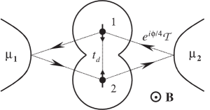
FIG. 2.: Double-dot (DD) system containing two electrons and being weakly coupled to metallic leads 1, 2, each of which is at the chemical potential $\mu_{1}$, $\mu_{2}$. The tunneling amplitudes between dots and leads are denoted by $\cal T$. The tunneling ($t_{d}$) between the dots results in a singlet-triplet splitting $J\sim t_{d}^{2}/U$ with the singlet being a ground state.[50] The tunneling path between dots and leads 1 and 2 forms a closed loop (shown by arrows) so that the Aharonov-Bohm phase $\phi$ will be accumulated by an electron traversing the DD.

We notice that for the noise power to be divergent the off-diagonal rates $w_{12}$ and $w_{21}$ have to vanish simultaneously. However, the matrix $w_{nm}$ is not symmetric since the off-diagonal rates depend on the bias in a different way. On the other hand, both rates contain the same matrix element of the cotunneling amplitude $(D^{{\dagger}}_{l},D_{l^{\prime}})$, see Eqs. (62) and (64). Although in general this matrix element is not small, it can vanish because of different symmetries of the two states. To illustrate this effect we consider the transport through a double-dot (DD) system (see Ref. [21] for details) as an example. Two leads are equally coupled to two dots in such a way that a closed loop is formed, and the dots are also connected, see Fig. 2. Thus, in a magnetic field the tunneling is described by the Hamiltonian Eq. (3) with

$$D_{l}=\sum_{s,j}T_{lj}c^{{\dagger}}_{ls}d_{js}\,,\qquad l,j=1,2\,,$$ (102)

$$T_{11}=T_{22}=T^{*}_{12}=T^{*}_{21}=e^{i\phi/4}{\cal T}\,,$$ (103)

where the last equation expresses the equal coupling of dots and leads and $\phi$ is the Aharonov-Bohm phase. Each dot contains one electron, and weak tunneling $t_{d}$ between the dots causes the exchange splitting[50] $J\sim t_{d}^{2}/U$ (with $U$ being the on-site repulsion) between one spin singlet and three triplets

$$|S\rangle=\frac{1}{\sqrt{2}}[d^{{\dagger}}_{1\uparrow}d^{{\dagger}}_{2\downarrow}\!-d^{{\dagger}}_{1\downarrow}d^{{\dagger}}_{2\uparrow}]|0\rangle\,,$$ (104)

$$|T_{0}\rangle=\frac{1}{\sqrt{2}}[d^{{\dagger}}_{1\uparrow}d^{{\dagger}}_{2\downarrow}\!+d^{{\dagger}}_{1\downarrow}d^{{\dagger}}_{2\uparrow}]|0\rangle\,,$$ (105)

$$|T_{+}\rangle=d^{{\dagger}}_{1\uparrow}d^{{\dagger}}_{2\uparrow}|0\rangle\,,\quad|T_{-}\rangle=d^{{\dagger}}_{1\downarrow}d^{{\dagger}}_{2\downarrow}|0\rangle\,.$$ (106)

In the case of zero magnetic field, $\phi=0$, the tunneling Hamiltonian $V$ is symmetric with respect to the exchange of electrons, $1\leftrightarrow 2$. Thus the matrix element of the cotunneling transition between the singlet and three triplets $\langle S|V(E-H_{0})^{-1}V|T_{i}\rangle$, $i=0,\pm$, vanishes because these states have different orbital symmetries. A weak magnetic field breaks the symmetry, contributes to the off-diagonal rates, and thereby reduces noise.

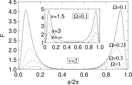
FIG. 3.: The Fano factor $F=S(\omega)/I$, with the noise power $S(\omega)$ given in Eqs. (92) and (112), and with the current through the DD, $I$, given in Eqs. (97) and (111), is plotted as a function of the Aharonov-Bohm phase $\phi$ for the normalized bias $v\equiv\Delta\mu/J=2$ and for four different normalized frequencies $\Omega\equiv\omega/[G(2\Delta\mu-J)]=0.1$, $0.25$, $0.5$, and $1$. Inset: the same, but with fixed frequency $\Omega=0.1$, where the bias $v$ takes the values $1.5$, $3$, and $\infty$.

The fact that in the perturbation $V$ all spin indices are traced out helps us to map the four-level system to only two states $|S\rangle$ and $|T\rangle$ classified according to the orbital symmetry (since all triplets are antisymmetric in orbital space). In Appendix C we derive the mapping to a two-level system and calculate the transition rates $w^{+}_{nm}$ and $w^{0}_{nm}$ ($n,m=1$ for a singlet and $n,m=2$ for all triplets) using Eqs. (62) and (64) with the operators $D_{l}$ given by Eq. (102). Doing this we obtain the following result

$$w^{0}_{nm}=0,$$ (107)

$$w^{+}_{nm}=\frac{\pi}{2}\left(\frac{\nu{\cal T}^{2}}{\Delta_{-}}\right)^{2}$$ (108)

$$\times\left\{\begin{array}[]{ll}(1\!+\!\cos\phi)\Delta\mu&(1\!-\!\cos\phi)(\Delta\mu\!+\!J)\\ 3(1\!-\!\cos\phi)(\Delta\mu\!-\!J)&3(1\!+\!\cos\phi)\Delta\mu\\ \end{array}\right\},$$ (111)

which holds close to the sequential tunneling peak, $\Delta_{-}\ll\Delta_{+}\sim U$ (but still $\Delta_{-}\gg J,\Delta\mu$), and for $\Delta\mu>J$. We substitute this equation into the Eq. (99) and write the correction $\Delta S(\omega)$ to the Poissonian noise as a function of normalized bias $v=\Delta\mu/J$ and normalized frequency $\Omega=e\omega/[G(2\Delta\mu-J)]$

$$\Delta S(\omega)=6eGJ\frac{(v^{2}-1)[1+(v-1)\cos\phi]^{2}(1-\cos\phi)}{(2v-1)^{3}[\Omega^{2}+(1-\cos\phi)^{2}]},$$ (112)

where $G=\pi e(\nu{\cal T}^{2}/\Delta_{-})^{2}$ is the conductance of a single dot in the cotunneling regime.[51] From Eq. (112) it follows that the noise power has singularities as a function of $\omega$ for zero magnetic field, and it has singularities at $\phi=2\pi m$ (where $m$ is integer) as a function of the magnetic field (see Fig. 3). We would like to emphasize that the noise is singular even if the exchange between the dots is weak, $J\ll\Delta\mu$. Note however, that our classical approach, which neglects the off-diagonal elements of the density matrix $\rho(t)$, can only be applied for weak enough tunneling, $w_{nm}\ll J$. In the case $\Delta\mu<J$ the transition from the singlet to the triplet is forbidden by conservation of energy, $w^{+}_{21}=0$, and we immediately obtain from Eq. (99) that $\Delta S(\omega)=0$, i.e. the total noise is Poissonian (as it is always the case for elastic cotunneling). In the case of large bias, $\Delta\mu\gg J$, two dots contribute independently to the current $I=2e^{-1}G\Delta\mu$, and from Eq. (112) we obtain the Fano factor

$$F=\frac{3}{8}\,\frac{\cos^{2}\!\phi(1-\cos\phi)}{\Omega^{2}+(1-\cos\phi)^{2}},\quad\Delta\mu\gg J.$$ (113)

This Fano factor controls the transition to the telegraph noise and then to the equilibrium noise at high temperature, as described above. We notice that if the coupling of the dots to the leads is not equal, then $w^{0}_{nm}\neq 0$ serves as a cut-off of the singularity in $\Delta S(\omega)$.

Finally, we remark that the Fano factor is a periodic function of the phase $\phi$ (see Fig. 3); this is nothing but an Aharonov-Bohm effect in the noise of the cotunneling transport through the DD. However, in contrast to the Aharonov-Bohm effect in the cotunneling current through the DD which has been discussed earlier in Ref. [21], the noise effect does not allow us to probe the ground state of the DD, since the DD is already in a mixture of the singlet and three triplet states.

VI Cotunneling through continuum of single-electron states

We consider now the transport through a multi-level QDS with $\delta E\ll E_{C}$. In the low bias regime, $\Delta\mu\ll(\delta E\,E_{C})^{1/2}$, the elastic cotunneling dominates transport,[25] and according to the results of Secs. IV and V the noise is Poissonian. Here we consider the opposite regime of inelastic cotunneling, $\Delta\mu\gg(\delta E\,E_{C})^{1/2}$. Since a large number $M$ of levels participate in transport, we can neglect the correlations which we have studied in the previous section, since they become a $1/M$-effect. Instead, we concentrate on the heating effect, which is not relevant for the 2-level system considered before. The condition for strong cotunneling has to be rewritten in a single-particle form, $\tau_{\rm in}\gg\tau_{c}$, where $\tau_{\rm in}$ is the single-particle energy relaxation time on the QDS due to the coupling to the environment, and $\tau_{c}$ is the time of the cotunneling transition, which can be estimated as $\tau_{c}\sim e\nu_{D}\Delta\mu/I$ (where $\nu_{D}$ is the density of QDS states). Since the energy relaxation rate on the QDS is small, the multiple cotunneling transitions can cause high energy excitations on the dot, and this leads to a nonvanishing backward tunneling, $w^{-}_{nm}\neq 0$. In the absence of correlations between cotunneling events, Eqs. (75), (76) and (92) can be rewritten in terms of forward and backward tunneling currents $I_{+}$ and $I_{-}$,

$$I=I_{+}-I_{-}\,,\quad S=e(I_{+}+I_{-}),$$ (114)

$$I_{\pm}=e\sum_{n,m}w^{\pm}_{nm}\bar{\rho}_{m}\,,$$ (115)

where the transition rates are given by Eqs. (59) and (62).

It is convenient to rewrite the currents $I_{\pm}$ in a single-particle basis. To do so we substitute the rates Eq. (62) into Eq. (115) and neglect the dependence of the tunneling amplitudes Eq. (3) on the quantum numbers $k$ and $p$, $T_{lkp}\equiv T_{l}$, which is a reasonable assumption for QDS with a large number of electrons. Then we define the distribution function on the QDS as

$$f(\varepsilon)=\nu_{D}^{-1}\sum_{p}\delta(\varepsilon-\varepsilon_{p}){\rm Tr}\,\bar{\rho}d^{{\dagger}}_{p}d_{p}$$ (116)

and replace the summation over $p$ with an integration over $\varepsilon$. Doing this we obtain the following expressions for $T=0$

$$I_{\pm}=C_{\pm}\frac{G_{1}G_{2}}{2\pi e^{3}}\left(\frac{1}{\Delta_{+}}+\frac{1}{\Delta_{-}}\right)^{2}(\Delta\mu)^{3},$$ (117)

$$C_{\pm}=\frac{1}{\Delta\mu^{3}}\int\!\!\int\!d\varepsilon d\varepsilon^{\prime}\Theta(\varepsilon\!-\varepsilon^{\prime}\!\pm\Delta\mu)f(\varepsilon)[1-f(\varepsilon^{\prime})],$$ (118)

where $G_{1,2}=\pi e^{2}\nu\nu_{D}|T_{1,2}|^{2}$ are the tunneling conductances of the two barriers, and where we have introduced the function $\Theta(\varepsilon)=\varepsilon\theta(\varepsilon)$ with $\theta(\varepsilon)$ being the step-function. In particular, using the property $\Theta(\varepsilon+\Delta\mu)-\Theta(\varepsilon-\Delta\mu)=\varepsilon+\Delta\mu$ and fixing

$$\int d\varepsilon[f(\varepsilon)-\theta({-\varepsilon})]=0,$$ (119)

(since $I_{\pm}$ given by Eq. (117) and Eq. (118) do not depend on the shift $\varepsilon\to\varepsilon+const$) we arrive at the following general expression for the cotunneling current

$$I=\Lambda\,\frac{G_{1}G_{2}}{12\pi e^{3}}\left(\frac{1}{\Delta_{+}}+\frac{1}{\Delta_{-}}\right)^{2}(\Delta\mu)^{3},$$ (120)

$$\Lambda=1+12\Upsilon/(\Delta\mu)^{2},$$ (121)

$$\Upsilon=\int d\varepsilon\varepsilon[f(\varepsilon)-\theta(-\varepsilon)]\geq 0,$$ (122)

where the value $\nu_{D}\Upsilon$ has the physical meaning of the energy acquired by the QDS due to the cotunneling current through it.

We have deliberately introduced the functions $C_{\pm}$ in the Eq. (117) to emphasize the fact that if the distribution $f(\varepsilon)$ scales with the bias $\Delta\mu$ (i.e. $f$ is a function of $\varepsilon/\Delta\mu$), then $C_{\pm}$ become dimensionless universal numbers. Thus both, the prefactor $\Lambda$ [given by Eq. (121)] in the cotunneling current, and the Fano factor $F=S/(eI)$, where $S=eI+\Delta S_{h}$,

$$F=\frac{C_{+}+C_{-}}{C_{+}-C_{-}},$$ (123)

take their universal values, which do not depend on the bias $\Delta\mu$. We consider now such universal regimes. The first example is the case of weak cotunneling, $\tau_{\rm in}\ll\tau_{c}$, when the QDS is in its ground state, $f(\varepsilon)=\theta(-\varepsilon)$, and the thermal energy of the QDS vanishes, $\Upsilon=0$. Then $\Lambda=1$, and Eq. (120) reproduces the results of Ref. [25]. As we have already mentioned, the backward current vanishes, $I_{-}=0$, and the Fano factor acquires its full Poissonian value $F=1$, in agreement with our nonequilibrium FDT proven in Sec. III B. In the limit of strong cotunneling, $\tau_{\rm in}\gg\tau_{c}$, the energy relaxation on the QDS can be neglected. Depending on the electron-electron scattering time $\tau_{ee}$ two cases have to be distinguished: The regime of cold electrons $\tau_{ee}\gg\tau_{c}$ and regime of hot electrons $\tau_{ee}\ll\tau_{c}$ on the QDS. Below we discuss both regimes in detail and demonstrate their universality.

A Cold electrons

In this regime the electron-electron scattering on the QDS can be neglected and the distribution $f(\varepsilon)$ has to be found from the master equation Eq. (57). We multiply this equation by $\nu_{D}^{-1}\sum_{p}\delta(\varepsilon-\varepsilon_{p})\langle n|d^{{\dagger}}_{p}d_{p}|n\rangle$, sum over $n$ and use the tunneling rates from Eq. (62). Doing this we obtain the standard stationary kinetic equation which can be written in the following form

$$\int d\varepsilon^{\prime}\sigma(\varepsilon^{\prime}-\varepsilon)f(\varepsilon^{\prime})[1-f(\varepsilon)]$$ (124)

$$\qquad\qquad\qquad=\int d\varepsilon^{\prime}\sigma(\varepsilon-\varepsilon^{\prime})f(\varepsilon)[1-f(\varepsilon^{\prime})],$$ (125)

$$\sigma(\varepsilon)=2\lambda\Theta(\varepsilon)+\sum_{\pm}\Theta(\varepsilon\pm\Delta\mu),$$ (126)

where $\lambda=(G_{1}^{2}+G_{2}^{2})/(2G_{1}G_{2})\geq 1$ arises from the equilibration rate $w^{0}_{mn}$, see Eq. (60). (We assume that if the limits of the integration over energy $\varepsilon$ are not specified, then the integral goes from $-\infty$ to $+\infty$.) From the form of this equation we immediately conclude that its solution is a function of $\varepsilon/\Delta\mu$, and thus the cold electron regime is universal as defined in the previous section. It is easy to check that the detailed balance does not hold, and in addition $\sigma(\varepsilon)\neq\sigma(-\varepsilon)$. Thus we face a difficult problem of solving Eq. (125) in its full nonlinear form. Fortunately, there is a way to avoid this problem and to reduce the equation to a linear form which we show next.

We group all nonlinear terms on the rhs of Eq. (125): $\int d\varepsilon^{\prime}\sigma(\varepsilon^{\prime}-\varepsilon)f(\varepsilon^{\prime})=h(\varepsilon)f(\varepsilon)$, where $h(\varepsilon)=\int d\varepsilon^{\prime}\left\{\sigma(\varepsilon^{\prime}-\varepsilon)f(\varepsilon^{\prime})+\sigma(\varepsilon-\varepsilon^{\prime})[1-f(\varepsilon^{\prime})]\right\}$. The trick is to rewrite the function $h(\varepsilon)$ in terms of known functions. For doing this we split the integral in $h(\varepsilon)$ into two integrals over $\varepsilon^{\prime}>0$ and $\varepsilon^{\prime}<0$, and then use Eq. (119) and the property of the kernel $\sigma(\varepsilon)-\sigma(-\varepsilon)=2(1+\lambda)\varepsilon$ to regroup terms in such a way that $h(\varepsilon)$ does not contain $f(\varepsilon)$ explicitly. Taking into account Eq. (122) we arrive at the following linear integral equation

$$\int d\varepsilon^{\prime}\sigma(\varepsilon^{\prime}-\varepsilon)f(\varepsilon^{\prime})$$ (127)

$$\qquad\qquad\qquad=[(1+\lambda)(\varepsilon^{2}+2\Upsilon)+(\Delta\mu)^{2}]f(\varepsilon),$$ (128)

where the parameter $\Upsilon$ is the only signature of the nonlinearity of Eq. (125).

Since Eq. (128) represents an eigenvalue problem for a linear operator, it can in general have more than one solution. Here we demonstrate that there is only one physical solution, which satisfies the conditions

$$0\leq f(\varepsilon)\leq 1,\quad f(-\infty)=1,\quad f(+\infty)=0.$$ (129)

Indeed, using a standard procedure one can show that two solutions of the integral equation (128), $f_{1}$ and $f_{2}$, corresponding to different parameters $\Upsilon_{1}\neq\Upsilon_{2}$ should be orthogonal, $\int d\varepsilon f_{1}(\varepsilon)f_{2}(-\varepsilon)=0$. This contradicts the conditions Eq. (129). The solution is also unique for the same $\Upsilon$, i.e. it is not degenerate (for a proof, see Appendix D). From Eq. (125) and conditions Eq. (129) it follows that if $f(\varepsilon)$ is a solution then $1-f(-\varepsilon)$ also satisfies Eqs. (125) and (129). Since the solution is unique, it has to have the symmetry $f(\varepsilon)=1-f(-\varepsilon)$.

FIG. 4.: The prefactor $\Lambda$ in the expression (120) for the cotunneling current characterizes a universal cotunneling transport in the regime of weak cotunneling, $\tau_{\rm in}\ll\tau_{c}$, ($\Lambda=1$, see Ref. [25]), and in the regime of strong cotunneling, $\tau_{\rm in}\gg\tau_{c}$ ($\Lambda>1$). Here $\Lambda$ is plotted as a function of $G_{1}/G_{2}$ (same as a function of $G_{2}/G_{1}$) for the strong cotunneling, for the cold-electron case, $\tau_{ee}\gg\tau_{c}$ (solid line) and for the hot-electron case, $\tau_{ee}\ll\tau_{c}$ (dotted line). $G_{1,2}$ are the tunneling conductances of a junctions connecting leads 1 and 2 with the QDS.

We solve Eqs. (128) and (129) numerically and use Eqs. (118) and (123) to find that the Fano factor is very close to 1 (it does not exceed the value $F\approx 1.006$). Next we use Eqs. (121) and (122) to calculate the prefactor $\Lambda$ and plot the result as a function of the ratio of tunneling conductances, $G_{1}/G_{2}$, (Fig. 4, solid line). For equal coupling to the leads, $G_{1}=G_{2}$, the prefactor $\Lambda$ takes its maximum value $2.173$, and thus the cotunneling current is approximately twice as large compared to its value for the case of weak cotunneling, $\tau_{\rm in}\ll\tau_{c}$. $\Lambda$ slowly decreases with increasing asymmetry of coupling and tends to its minimum value $\Lambda=1$ for the strongly asymmetric coupling case $G_{1}/G_{2}orG_{2}/G_{1}\gg 1$.

B Hot electrons

In the regime of hot electrons, $\tau_{ee}\ll\tau_{c}$, the distribution is given by the equilibrium Fermi function $f_{F}(\varepsilon)=\left[1+\exp(\varepsilon/k_{B}T_{e})\right]^{-1}$, while the electron temperature $T_{e}$ has to be found self-consistently from the kinetic equation. Eq. (125) has to be modified to take into account electron-electron interactions. This can be done by adding the electron collision integral $I_{ee}(\varepsilon)$ to the rhs. of (125). Since the form of the distribution is known we need only the energy balance equation, which can be derived by multiplying the modified equation (125) by $\varepsilon$ and integrating it over $\varepsilon$. The contribution from the collision integral $I_{ee}(\varepsilon)$ vanishes, because the electron-electron scattering conserves the energy of the system. Using the symmetry $f_{F}(\varepsilon)=1-f_{F}(-\varepsilon)$ we arrive at the following equation

$$\int\!\!\int d\varepsilon d\varepsilon^{\prime}f_{F}(\varepsilon^{\prime})[1-f_{F}(\varepsilon)]\sigma(\varepsilon^{\prime}-\varepsilon)\varepsilon=0.$$ (130)

Next we regroup the terms in this equation such that it contains only integrals of the form $\int_{0}^{\infty}d\varepsilon f_{F}(\varepsilon)(\ldots)$. This allows us to get rid of nonlinear terms, and we arrive at the following equation,

$$\int d\varepsilon\varepsilon^{3}[f_{F}(\varepsilon)-\theta(-\varepsilon)]+3\Upsilon^{2}=\frac{(\Delta\mu)^{4}}{8(1+\lambda)}\,,$$ (131)

which holds also for the regime of cold electrons. Finally, we calculate the integral in Eq. (131) and express the result in terms of the dimensionless parameter $\alpha=\Delta\mu/k_{B}T_{e}$,

$$\alpha=\pi\left[8(1+\lambda)/5\right]^{1/4}.$$ (132)

Thus, since the distribution again depends on the ratio $\varepsilon/\Delta\mu$, the hot electron regime is also universal.

The next step is to substitute the Fermi distribution function with the temperature given by Eq. (132) into Eq. (118). We calculate the integrals and arrive at the closed analytical expressions for the values of interest,

$$\Lambda=1+\frac{2\pi^{2}}{\alpha^{2}}=1+\sqrt{\frac{5}{2(1+\lambda)}}\,,$$ (133)

$$F=1+\frac{12}{2\pi^{2}+\alpha^{2}}\sum_{n=1}^{\infty}\left[\frac{1}{n^{2}}+\frac{2}{\alpha n^{3}}\right]e^{-\alpha n},$$ (134)

where again $\lambda=(G_{1}^{2}+G_{2}^{2})/2G_{1}G_{2}\geq 1$. It turns out that similar to the case of cold electrons, Sec. VI A, the Fano factor for hot electrons is very close to $1$ (namely, it does not exceed the value $F\approx 1.007$). Therefore, we do not expect that the super-Poissonian noise considered in this section (i.e. the one which is due to heating of a large QDS caused by inelastic cotunneling through it) will be easy to observe in experiments. On the other hand, the transport-induced heating of a large QDS can be observed in the cotunneling current through the prefactor $\Lambda$, which according to Eq. (133) takes its maximum value $\Lambda=1+\sqrt{5/4}\approx 2.118$ for $G_{1}=G_{2}$ and slowly reaches its minimum value $1$ with increasing (or decreasing) the ratio $G_{1}/G_{2}$ (see Fig. 4, dotted line). Surprisingly, the two curves of $\Lambda$ vs $G_{1}/G_{2}$ for the cold- and hot-electron regimes lie very close, which means that the effect of the electron-electron scattering on the cotunneling transport is rather weak.

VII Conclusions

The physics of the noise of cotunneling is discussed in the Introduction. Here we give a short summary of our results.

In Sec. III, we have derived the non-equilibrium FDT, i.e. the universal relations Eqs. (19) and (34) between the current and the noise, for single-barrier junctions and for QDS in the weak cotunneling regime, respectively. Taking the limit $T,\omega\rightarrow 0$, we show that the noise is Poissonian, i.e. $F=1$.

In Sec. IV, we have derived the master equation, Eq. (57), the stationary state Eq. (66) of the QDS, the average current, Eq. (75), and the current correlators, Eqs. (91)-(93) for a non-degenerate QDS system ($E_{n}\neq E_{m}$, $n\neq m$) coupled to leads in the strong cotunneling regime $w_{\rm in}\ll w$ at small frequencies, $\omega\ll\Delta_{mn}$. In contrast to sequential tunneling, where shot noise is either Poissonian ($F=1$) or suppressed due to charge conservation ($F<1$), we find that the noise in the inelastic cotunneling regime can be super-Poissonian ($F>1$), with a correction being as large as the Poissonian noise itself. In the regime of elastic cotunneling $F=1$.

While the amount of super-Poissonian noise is merely estimated at the end of Sec. IV, the noise of the cotunneling current is calculated for the special case of a QDS with nearly degenerate states, i.e. $\Delta_{nm}\ll\delta E$, in Sec. V, where we apply our results from Sec. IV. The general solution Eq. (96) is further analyzed for two nearly degenerate levels, with the result Eq. (99). More information is gained in the specific case of a DD coupled to leads, where we determine the correction to noise Eq. (112) as a function of frequency, bias, and the Aharonov-Bohm phase threading the tunneling loop, finding signatures of the Aharonov-Bohm effect in the cotunneling noise.

Finally, in Sec. VI, another important situation is studied in detail, the cotunneling through a QDS with a continuous energy spectrum, $\delta E\ll\Delta\mu\ll E_{C}$. Here, the correlation between tunneling events plays a minor role as a source of super-Poissonian noise, which is now caused by heating effects opening the possibility for tunneling events in the reverse direction and thus to an enhanced noise power. In Eq. (123), we express the Fano factor $F$ in the continuum case in terms of the dimensionless numbers $C_{\pm}$, defined in Eq. (118), which depend on the electronic distribution function $f(\varepsilon)$ in the QDS (in this regime, a description on the single-electron level is appropriate). The current Eq. (120) is expressed in terms of the prefactor $\Lambda$, Eq. (121). Both $F$ and $\Lambda$ are then calculated for different regimes. For weak cotunneling, we immediately find $F=1$, as anticipated earlier, while for strong cotunneling we distinguish the two regimes of cold ($\tau_{ee}\gg\tau_{c}$) and hot ($\tau_{ee}\ll\tau_{c}$) electrons. For cold electrons, we derive the linear integral equation Eq. (128) for $f(\varepsilon)$ which is shown to have a unique solution, and which is solved numerically. We find that the Fano factor is very close to one, $1<F<1.006$, while $\Lambda$ is given in Fig. 4. For hot electrons, $f(\varepsilon)$ is the equilibrium Fermi distribution, and the Fano factor Eq. (134) and $\Lambda$ [Eq. (133)and Fig. 4] can be computed analytically. Again, the Fano factor is very close to one, $1<F<1.007$, which leads us to the conclusion that heating will hardly be observed in noise, but should be well measurable in the cotunneling current.

A

In this Appendix we present the derivation of Eqs. (24) and (26). First we would like to mention that the operator $B$ in these equations is just the second-order tunneling amplitude, which also appears in the tunneling Hamiltonian after the Schrieffer-Wolff transformation. Therefore, one might think that the Schrieffer-Wolff transformation is the most simple way to derive Eqs. (24) and (26). On the other hand, it is obvious that the Schrieffer-Wolff procedure being a unitary transformation gives exactly the same amount of terms in the fourth-order expression for the current and noise as that of the regular perturbation expansion. The Schrieffer-Wolff procedure is useful in the Kondo regime where the energy scale is given by the Kondo temperature $T_{K}$ and where the $B$-terms in the Hamiltonian lead to a divergence for $T<T_{K}$, while the other terms can be treated by perturbation theory (see Ref. [52]). In our cotunneling regime such a divergence does not exist (since the QDS is weakly coupled to leads, i.e. $\Delta\mu,k_{B}T\gg k_{B}T_{K}$), and we have to analyze all contributions. We do this below using perturbation theory.

In order to simplify the intermediate steps, we use the notation $\bar{O}(t)\equiv\int_{-\infty}^{t}dt^{\prime}O(t^{\prime})$ for any operator $O$, and $O(0)\equiv O$. We notice that, if an operator $O$ is a linear function of operators $D_{l}$ and $D_{l}^{{\dagger}}$, then $\bar{O}(\infty)=0$ (see the discussion in Sec. III B). Next, the currents can be represented as the difference and the sum of $\hat{I}_{1}$ and $\hat{I}_{2}$,

$$\hat{I}_{d} = (\hat{I}_{2}-\hat{I}_{1})/2=ie(X^{{\dagger}}-X)/2\,,$$ (A1)

$$\hat{I}_{s} = (\hat{I}_{1}+\hat{I}_{2})/2=ie(Y^{{\dagger}}-Y)/2\,,$$ (A2)

where $X=D_{2}+D_{1}^{{\dagger}}$, and $Y=D_{1}+D_{2}$. While for the perturbation we have

$$V=X+X^{{\dagger}}=Y+Y^{{\dagger}}\,.$$ (A3)

First we concentrate on the derivation of Eq. (24) and redefine the average current Eq. (7) as $I=I_{d}$ (which gives the same result anyway, because the average number of electrons on the QDS does not change $I_{s}=0$).

To proceed with our derivation, we make use of Eq. (8) and expand the current up to fourth order in $T_{lkp}$:

$$I = i\int\limits^{0}_{-\infty}dt\int\limits^{t}_{-\infty}dt^{\prime}\langle\hat{I}_{d}V(t)V(t^{\prime})\bar{V}(t^{\prime})\rangle$$ (A4)

$$- i\int\limits^{0}_{-\infty}dt\langle\bar{V}\hat{I}_{d}V(t)\bar{V}(t)\rangle+{\rm c.c.}\,$$ (A5)

Next, we use the cyclic property of trace to shift the time dependence to $\hat{I}_{d}$. Then we complete the integral over time $t$ and use $\bar{I}_{d}(\infty)=0$. This procedure allows us to combine first and second term in Eq. (A5),

$$I=-i\int\limits^{0}_{-\infty}dt\langle[\bar{I}_{d}V+\bar{V}\hat{I}_{d}]V(t)\bar{V}(t)\rangle+{\rm c.c.}\,$$ (A6)

Now, using Eqs. (A1) and (A3) we replace operators in Eq. (A6) with $X$ and $X^{{\dagger}}$ in two steps: $I=e\int^{0}_{-\infty}dt\langle[\bar{X}^{{\dagger}}X^{{\dagger}}-\bar{X}X]V(t)\bar{V}(t)\rangle+{\rm h.c.}$, where some terms cancel exactly. Then we work with $V(t)\bar{V}(t)$ and notice that some terms cancel, because they are linear in $c_{lk}$ and $c_{lk}^{{\dagger}}$. Thus we obtain

$$I=e\int\limits^{0}_{-\infty}dt \langle[\bar{X}^{{\dagger}}X^{{\dagger}}-\bar{X}X]$$ (A8)

$$\times[X^{{\dagger}}(t)\bar{X}^{{\dagger}}(t)+X(t)\bar{X}(t)]\rangle+{\rm c.c.}\,$$

Two terms $\bar{X}XX\bar{X}$ and $\bar{X}^{{\dagger}}X^{{\dagger}}X^{{\dagger}}\bar{X}^{{\dagger}}$ describe tunneling of two electrons from the same lead, and therefore they do not contribute to the normal current. We then combine all other terms to extend the integral to $+\infty$,

$$I=e\int\limits^{\infty}_{-\infty}dt\langle\bar{X}^{{\dagger}}(t)X^{{\dagger}}(t)X\bar{X}-\bar{X}XX^{{\dagger}}(t)\bar{X}^{{\dagger}}(t)\rangle\,$$ (A9)

Finally, we use $\int^{\infty}_{-\infty}dtX(t)\bar{X}(t)=-\int^{\infty}_{-\infty}dt\bar{X}(t)X(t)$ (since $\bar{X}(\infty)=0$) to get Eq. (24) with $B=X\bar{X}$. Here, again, we drop terms $D^{{\dagger}}_{1}\bar{D}^{{\dagger}}_{1}$ and $D_{2}\bar{D}_{2}$ responsible for tunneling of two electrons from the same lead, and obtain $B$ as in Eq. (25).

Next, we derive Eq. (26) for the noise power. At small frequencies $\omega\ll\Delta_{\pm}$ fluctuations of $I_{s}$ are suppressed because of charge conservation (see below), and we can replace $\hat{I}_{2}$ in the correlator Eq. (7) with $\hat{I}_{d}$. We expand $S({\omega})$ up to fourth order in $T_{lkp}$, use $\int_{-\infty}^{+\infty}dt\,\hat{I}_{d}(t)e^{\pm i\omega t}=0$, and repeat the steps leading to Eq. (A6). Doing this we obtain,

$$S(\omega)=-\int\limits^{\infty}_{-\infty}dt\cos(\omega t)\langle[\bar{V}(t),\hat{I}_{d}(t)][\bar{V},\hat{I}_{d}]\rangle\,.$$ (A10)

Then, we replace $V$ and $\hat{I}_{d}$ with $X$ and $X^{{\dagger}}$. We again keep only terms relevant for cotunneling, and in addition we neglect terms of order $\omega/\Delta_{\pm}$ (applying same arguments as before, see Eq. (A11)). We then arrive at Eq. (26) with the operator $B$ given by Eq. (25).

Finally, in order to show that fluctuations of $I_{s}$ are suppressed, we replace $\hat{I}_{d}$ in Eq. (A10) with $\hat{I}_{s}$, and then use the operators $Y$ and $Y^{{\dagger}}$ instead of $X$ and $X^{{\dagger}}$. In contrast to Eq. (A9) terms such as $\bar{Y}^{{\dagger}}Y^{{\dagger}}Y\bar{Y}$ do not contribute, because they contain integrals of the form $\int^{\infty}_{-\infty}dt\cos(\omega t)D_{l}(t)\bar{D}_{l^{\prime}}(t)=0$. The only nonzero contribution can be written as

$$S_{ss}(\omega)=\frac{e^{2}\omega^{2}}{4}\int\limits^{\infty}_{-\infty}dt\cos(\omega t)\langle[\bar{Y}^{{\dagger}}(t),\bar{Y}(t)][\bar{Y}^{{\dagger}},\bar{Y}]\rangle\,,$$ (A11)

where we have used integration by parts and the property $\bar{Y}(\infty)=0$. Compared to Eq. (26) this expression contains an additional integration over $t$, and thereby it is of order $(\omega/\Delta_{\pm})^{2}$.

B

We evaluate the matrix elements of the superoperator $W^{I}(z)$ given in Eq. (71) which are used to calculate the average current $I_{l}$, see Eq. (75). The derivation for the master equation (57) is very similar. As for the noise, the $S^{Q}_{ll^{\prime}}$ term Eq. (90) is again obtained in a similar way as the current, whereas the $S^{P}_{ll^{\prime}}$ term Eq. (85) is different and is analyzed in Sec. IV E. Since $W^{I}(z)$ is obtained by taking the partial trace over the leads, its matrix elements can be expressed as the sum over lead indices

$$W^{I}_{nm}(z)=\sum_{\bar{n}\bar{m}}{\cal W}^{I}_{\bf nm}(z)\,\rho_{L,\bar{m}}(z),$$ (B1)

where ${\bf n}=(n,\bar{n})$, with $n$ and $\bar{n}$ enumerating the QDS and lead eigenstates. For convenience, we will use the eigenstates of $H_{0}$ in this Appendix, and not the eigenstates of $K$ as in the main text. Accordingly, here $E_{\bf n}=E_{n}+E_{\bar{n}}$ are the eigenenergies of $H_{0}$. Taking the stationary limit $z\rightarrow 0$, using the definition Eq. (71) and introducing the projectors $p_{\bf n}=|{\bf n}\rangle\langle{\bf n}|$, we can write

$${\cal W}^{I}_{\bf nm}=\lim_{z\rightarrow 0}{\rm Tr}\,p_{\bf n}\hat{I}_{l}Q\frac{1}{z-QLQ}QL_{V}Pp_{\bf m}.$$ (B2)

Note that while ${\bf n}$ denotes a free dummy index in Eq. (B2), the state $|{\bf m}\rangle$ is restricted to the subspace where $P_{N}p_{\bf m}\neq 0$ with fixed particle number $N$ on the QDS. Expanding this expression in $V$, we obtain for the lowest nonvanishing order (sequential tunneling) the contribution $-i\sum_{\bar{n}\bar{m}}(\hat{I}_{l}R_{0}L_{V}p_{\bf m})_{\bf nn}$ to the rate $W^{I}_{nm}$, which can be expressed as

$$2\pi e\sum_{\bar{n}\bar{m}}\left(|\langle{\bf n}|D_{l}|{\bf m}\rangle|^{2}-|\langle{\bf n}|D_{l}^{\dagger}|{\bf m}|\rangle|^{2}\right)\rho_{L,\bar{m}}\,\delta(\Delta_{\bf mn}),$$ (B3)

where $\Delta_{\bf mn}=E_{\bf m}-E_{\bf n}$. Using Eq. (3) and assuming that $T_{lkp}={\cal T}$ is independent of $p$ and $k$, we obtain the expression for the contribution to $W^{I}_{nm}$ due to sequential tunneling,

$$2\pi\nu{\cal T}^{2}\sum_{p}\left(|\langle n|d_{p}|m\rangle|^{2}\left[1-f_{l}(\Delta_{mn})\right]\right.$$ (B4)

$$\quad\quad\quad\left.-|\langle n|d_{p}^{\dagger}|m\rangle|^{2}f_{l}(\Delta_{nm})\right),$$ (B5)

where $f_{l}(\varepsilon)$ is the Fermi distribution and $\nu$ the density of states in the leads. In the cotunneling regime[37], this contribution is proportional to $\kappa=e^{-\Delta/k_{B}T}$, therefore we drop it[47] and expand $W^{I}_{nm}$ to the next non-vanishing, i.e. fourth, order in $V$. Doing this, we obtain the cotunneling contribution

$${\cal W}^{I}_{\bf nm}=i(\hat{I}_{l}R_{0}L_{V}R_{0}QL_{V}R_{0}L_{V}p_{\bf m})_{\bf nn}.$$ (B6)

Stepwise evaluation of the operators and superoperators in this expression by the insertion of the identity $\sum_{\bf i}|{\bf i}\rangle\langle{\bf i}|$ leads to

$${\cal W}^{I}_{\bf nm} = i\sum_{{\bf i},{\bf j}}(I_{\bf ni}R_{\bf in}V_{\bf ij}R_{\bf jn}U_{\bf jn}^{\bf m}-I_{\bf ni}R_{\bf in}R_{\bf ij}U_{\bf ij}^{\bf m}V_{\bf jn}),$$ (B7)

$$U_{\bf ij}^{\bf m} = (L_{V}R_{0}L_{V}p_{\bf m})_{\bf ij}$$ (B8)

$$= \sum_{\bf k}\left[V_{\bf ik}R_{\bf kj}(L_{V}p_{\bf m})_{\bf kj}-R_{\bf ik}(L_{V}p_{\bf m})_{\bf ik}V_{\bf kj}\right],$$ (B9)

$$(L_{V}p_{\bf m})_{\bf ij} = V_{\bf im}\delta_{\bf mj}-V_{\bf mj}\delta_{\bf im},$$ (B10)

where $I_{\bf ij}=\langle{\bf i}|\hat{I}_{l}|{\bf j}\rangle$, and similarly for $V_{\bf ij}$. Note that

$$R_{\bf ij} = \lim_{\eta\rightarrow 0}\frac{i}{i\eta-(E_{\bf i}-E_{\bf j})}$$ (B11)

$$= -i{\rm P}\frac{1}{E_{\bf i}-E_{\bf j}}+\pi\delta(E_{\bf i}-E_{\bf j}),$$ (B12)

where P stands for the principal value. The current $I_{l}$ is obtained from ${\cal W}^{I}_{\bf nm}$ by multiplying with the full density matrix $\rho_{\bf m}$ and then summing over ${\bf m}$ and ${\bf n}$. By explicit evaluation, using the fact that we can choose the basis $|n\rangle$ on the QDS such that all expectation values of the form $\langle n|d_{p_{1}}^{\dagger}d_{p_{2}}d_{p_{3}}^{\dagger}d_{p_{4}}|n\rangle$, etc., are real, we find that four out of the eight terms in Eq. (B10) cancel, while the remaining four terms contributing to the current $I_{l}$ can be combined into (retaining only $O(\kappa^{0})$ terms)

$$\sum_{\bf n}{\cal W}^{I}_{\bf nm} = -2\pi\,{\rm Im}\sum_{\bf f}\left[(\hat{I}_{l}R_{\bf m}^{\dagger}V)_{\bf mf}(VR_{\bf m}^{\dagger}V)_{\bf fm}\right.$$ (B14)

$$\left.+(VR_{\bf m}V)_{\bf mf}(\hat{I}_{l}R_{\bf f}^{\dagger}V)_{\bf fm}\right]\delta(E_{\bf f}-E_{\bf n}),$$

where $R_{\bf m}=-i{\rm P}(H_{0}-E_{\bf m})^{-1}$. All other $\delta$-function contributions vanish in $O(\kappa^{0})$. [47] In the presence of an Aharonov-Bohm phase, when the phases in the tunneling amplitudes Eq. (103) have to be taken into account, we again find Eq. (B14) by explicit analysis. We note here that exactly the same procedure as above can be applied in the derivation of the the master equation and the noise, leading to a reduction of terms and finally to the “golden rule” expressions Eqs. (58) and (90). By substituting Eqs. (3) and (6) for $V$ and $\hat{I}_{l}$, and setting $l=2$ for concreteness, we finally obtain

$$\sum_{\bf n}{\cal W}^{I}_{\bf nm} = 2\pi e\sum_{\bf f}\left[(D_{2}^{\dagger},D_{1})_{\bf mf}(D_{1}^{\dagger},D_{2})_{\bf fm}\right.$$ (B16)

$$\left.-(D_{1}^{\dagger},D_{2})_{\bf mf}(D_{2}^{\dagger},D_{1})_{\bf fm}\right]\delta(\Delta_{\bf fm}),$$

where $(D_{l}^{\dagger},D_{l^{\prime}})$ is defined in Eq. (64). Using Eqs. (71) and (B1) and the definitions Eqs. (59) and (62), we find for the cotunneling current

$$I_{2}=\sum_{\bf nm}{\cal W}^{I}_{\bf nm}\,\bar{\rho}_{m}\rho_{L,\bar{m}}=e\sum_{nm}(w^{+}_{nm}-w^{-}_{mn})\bar{\rho}_{m},$$ (B17)

which concludes the derivation of Eqs. (75) and (76). Note that in Eq. (62) the expression $\Delta_{\bf mn}=E_{\bf m}-E_{\bf n}$ is replaced by $E_{\bf m}-E_{\bf n}-\Delta\mu_{ll^{\prime}}$ because there, $|{\bf n}\rangle$ are eigenstates of $K$ (instead of $H_{0}$). The current $I_{1}$ in lead $1$ can be obtained by interchanging the lead indices $1$ and $2$ in Eq. (B16) which obviously leads to $I_{1}=-I_{2}$.

C

In this Appendix we calculate the transition rates Eq. (62) for a DD coupled to leads with the coupling described by Eqs. (102) and (103) and show that the four-level system in the singlet-triplet basis Eq. (105) can be mapped to a two-level system. For the moment we assume that the indices $n$ and $m$ enumerate the singlet-triplet basis, $n,m=S,T_{0},T_{+},T_{-}$. Close to the sequential tunneling peak, $\Delta_{-}\ll\Delta_{+}$, we keep only terms of the form $D^{{\dagger}}_{l}R_{0}D_{l}$. Calculating the trace over the leads explicitly, we obtain at $T=0$,

$$w_{nm}(l^{\prime},l) = \frac{\pi\nu^{2}}{2\Delta^{2}_{-}}\,\Theta(\mu_{l}-\mu_{l^{\prime}}-\Delta_{nm})$$ (C1)

$$\times \sum_{j,j^{\prime}}T^{*}_{lj}T_{lj^{\prime}}T^{*}_{l^{\prime}j^{\prime}}T_{l^{\prime}j}M_{nm}(j,j^{\prime})\,,$$ (C2)

$$M_{nm}(j,j^{\prime}) = \sum_{s,s^{\prime}}\langle n|d^{{\dagger}}_{sj}d_{s^{\prime}j}|m\rangle\langle m|d^{{\dagger}}_{s^{\prime}j^{\prime}}d_{sj^{\prime}}|n\rangle\,,$$ (C3)

with $\Theta(\varepsilon)=\varepsilon\theta(\varepsilon)$, and $\Delta_{nm}=0,\pm J$, and we have assumed $t_{d}\ll\Delta_{-}$ so that $R_{0}=1/\Delta_{-}$.

Since the quantum dots are the same we get $M_{nm}(1,1)=M_{nm}(2,2)$, and $M_{nm}(1,2)=M_{nm}(2,1)$. We calculate these matrix elements in the singlet-triplet basis explicitly,

$$M(1,1)=\frac{1}{2}\left(\begin{array}[]{rrrr}1&1&1&1\\ 1&1&1&1\\ 1&1&2&0\\ 1&1&0&2\end{array}\right),$$ (C8)

$$M(1,2)=\frac{1}{2}\left(\begin{array}[]{rrrr}1&-1&-1&-1\\ -1&1&1&1\\ -1&1&2&0\\ -1&1&0&2\end{array}\right).$$ (C13)

Assuming now equal coupling of the form Eq. (103) we find that for $l=l^{\prime}$ the matrix elements of the singlet-triplet transition vanish (as we have expected, see Sec. V). On the other hand the triplets are degenerate, i.e. $\Delta_{nm}=0$ in the triplet sector. Then from Eq. (C2) it follows that $w^{0}_{nm}=\sum_{l}w_{nm}(l,l)=0$. Next, we have $\Theta(\mu_{2}-\mu_{1}-\Delta_{nm})=0$, since for nearly degenerate states we assume $\Delta\mu>|\Delta_{nm}|$, and thus $w^{-}_{nm}=w_{nm}(1,2)=0$. Finally, for $w^{+}_{nm}=w_{nm}(2,1)$ we obtain,

$$w^{+}_{SS} = \frac{\pi}{2}\left(\frac{\nu{\cal T}^{2}}{\Delta_{-}}\right)^{2}\Delta\mu(1+\cos\phi),$$ (C14)

$$w^{+}_{ST} = \frac{\pi}{2}\left(\frac{\nu{\cal T}^{2}}{\Delta_{-}}\right)^{2}(\Delta\mu+J)(1-\cos\phi),$$ (C15)

$$w^{+}_{TS} = \frac{\pi}{2}\left(\frac{\nu{\cal T}^{2}}{\Delta_{-}}\right)^{2}(\Delta\mu-J)(1-\cos\phi),$$ (C16)

$$w^{+}_{TT} = \frac{\pi}{2}\left(\frac{\nu{\cal T}^{2}}{\Delta_{-}}\right)^{2}\Delta\mu$$ (C17)

$$\times \left(\begin{array}[]{lll}1+\cos\phi&1+\cos\phi&1+\cos\phi\\ 1+\cos\phi&2+2\cos\phi&0\\ 1+\cos\phi&0&2+2\cos\phi\end{array}\right).$$ (C21)

Next we prove the mapping to a two-level system. First we notice that because the matrix $w^{+}_{TT}$ is symmetric, the detailed balance equation for the stationary state gives $\bar{\rho}_{n}/\bar{\rho}_{m}=w^{+}_{mn}/w^{+}_{nm}=1$, $n,m\in T$. Thus we can set $\bar{\rho}_{n}\to\bar{\rho}_{2}/3$, for $n\in T$. The specific form of the transition matrix Eqs. (C14-C21) helps us to complete the mapping by setting $(1/3)\sum_{m=2}^{4}w^{+}_{1m}\to w^{+}_{12}$, $\sum_{n=2}^{4}w^{+}_{n1}\to w^{+}_{21}$, and $(1/3)\sum_{n,m=2}^{4}w^{+}_{nm}\to w^{+}_{22}$, so that we get the new transition matrix Eq. (111), while the stationary master equation for the new two-level density matrix does not change its form. If in addition we set $(1/3)\sum^{4}_{m=2}\delta\rho_{1m}(t)\to\delta\rho_{12}(t)$, $\sum^{4}_{n=2}\delta\rho_{n1}(t)\to\delta\rho_{21}(t)$, and $(1/3)\sum^{4}_{n,m=2}\delta\rho_{nm}(t)\to\delta\rho_{22}(t)$, then the master equation Eq. (57) for $\delta\rho_{nm}(t)$ and the initial condition $\delta\rho_{nm}(0)=\delta_{nm}-\bar{\rho}_{n}$ do not change either. Finally, one can see that under this mapping Eq. (93) for the correction to the noise power $\Delta S(\omega)$ remains unchanged. Thus we have accomplished the mapping of our singlet-triplet system to the two-level system with the new transition matrix given by Eq. (111).

D

Here we prove that the solution of Eqs. (128), (122), and (129) is not degenerate. Suppose the opposite is true, i.e. there are two functions, $f_{1}(\varepsilon)$ and $f_{2}(\varepsilon)$, which satisfy these equations. Then the function $f_{d}(\varepsilon)=f_{1}(\varepsilon)-f_{2}(\varepsilon)$ satisfies Eq. (128) with the conditions

$$\int d\varepsilon f_{d}(\varepsilon)=\int d\varepsilon\varepsilon f_{d}(\varepsilon)=0,$$ (D1)

$$f_{d}(+\infty)=f_{d}(-\infty)=0,\quad-1\leq f_{d}(\varepsilon)\leq 1.$$ (D2)

According to Eqs. (128), and (122), the integral $\int d\varepsilon|\varepsilon f_{d}(\varepsilon)|$ is convergent. This allows us to symmetrize the kernel $\sigma$ in Eq. (128): $\sigma(\varepsilon)=\sigma_{S}(\varepsilon)+(1+\lambda)\varepsilon+\Delta\mu$, where $\sigma_{S}(\varepsilon)=[\lambda\Theta(\varepsilon)+\Theta(\varepsilon-\Delta\mu)]+[\varepsilon\to-\varepsilon]$, and thus $\sigma_{S}(\varepsilon)=\sigma_{S}(-\varepsilon)$. Using the condition Eq. (D1) we arrive at the new integral equation for $f_{d}$,

$$\int d\varepsilon^{\prime}\sigma_{S}(\varepsilon^{\prime}-\varepsilon)f_{d}(\varepsilon^{\prime})$$ (D3)

$$\qquad\qquad\qquad=[(1+\lambda)(\varepsilon^{2}+2\Upsilon)+(\Delta\mu)^{2}]f_{d}(\varepsilon).$$ (D4)

Next we apply Fourier transformation to both sides of this equation and introduce the function

$$\varphi(x)=\frac{1}{2\pi}\int d\varepsilon e^{-i\varepsilon x}f_{d}(\varepsilon).$$ (D5)

Here we have to be careful because, strictly speaking the Fourier transform of $\sigma_{S}(\varepsilon)$ does not exist (this function is divergent at $\pm\infty$). On the other hand, since the integral on the lhs of Eq. (D4) is convergent, we can regularize the kernel as $\sigma_{S}(\varepsilon)\to\sigma_{S}(\varepsilon)e^{-\eta|\varepsilon|}$ and later take the limit $\eta\to+0$. Then for the Fourier transform of Eq. (D4) we find

$$(1+\lambda)\varphi^{\prime\prime}(x)=[u(x)+(\Delta\mu)^{2}+2(1+\lambda)\Upsilon]\varphi(x),$$ (D6)

$$u(x)=\int d\varepsilon e^{-i\varepsilon x}\sigma_{S}(\varepsilon)=2[\lambda+\cos(\Delta\mu x)]/x^{2},$$ (D7)

where $u(x)$ is real, because $\sigma_{S}$ is an even function of $\varepsilon$. Thus we have obtained a second order differential (Schrödinger) equation for the function $\varphi(x)$. We conclude from Eq. (D1) that $\varphi(0)=\varphi^{\prime}(0)=0$, and the condition Eq. (D2) ensures that the solution of Eq. (D6) is localized, $\varphi(x)|_{x\to\pm\infty}=0$ and finite everywhere. All these requirements can be satisfied only if $\varphi(x)=0$ for all $x$. Indeed, since the function $u(x)+(\Delta\mu)^{2}+2(1+\lambda)\Upsilon$ is positive for all $x$ (we recall that $\Upsilon>0$), then $\varphi$ is a monotonous function, and therefore it cannot be localized. In other words, the Schrödinger equation with repulsive potential $u(x)>0$ does not have localized solutions. Thus we have proven that $f_{1}(\varepsilon)=f_{2}(\varepsilon)$ for all $\varepsilon$, and the solution of Eq. (128) is not degenerate.

REFERENCES

• [1] L.P. Kouwenhoven, G. Schön, L. L. Sohn, Mesoscopic Electron Transport, NATO ASI Series E:Applied Sciences-Vol. 345, (Kluwer Academic, Dordrecht, 1997).
• [2] See, e.g., Electron transport in quantum dots, L. P. Kouwenhoven et al., in Ref. [1].
• [3] For a review, see: M. H. Devoret, and R. J. Schoelkopf, Nature 406, 1039 (2000).
• [4] A. N. Korotkov, D. V. Averin, K. K. Likharev, and S. A. Vasenko, in Single-Electron Tunneling and Mesoscopic Devices, ed. by H. Koch and H. Lübbig, Springer Series in Electronics and Photonics, Vol. 31, p. 45 (Springer-Verlag, Berlin, 1992).
• [5] A. N. Korotkov, Phys. Rev. B 49, 10381 (1994).
• [6] For a recent review on shot noise, see: Ya. M. Blanter and M. Büttiker, Shot Noise in Mesoscopic Conductors, Phys. Rep. 336, 1 (2000); [cond-mat/9910158].
• [7] S. Hershfield et al., Phys. Rev. B 47, 1967 (1993).
• [8] Yu. M. Galperin et al., Mod. Phys. Lett. B 7, 1159 (1993).
• [9] U. Hanke, et al., Phys. Rev. B 48, 17209 (1993).
• [10] U. Hanke, et al., Phys. Rev. B 50, 1595 (1994).
• [11] W. Krech, A. Hädicke, and H.-O. Müller, Int. J. Mod. Phys. B 6, 3555 (1992).
• [12] W. Krech, and H.-O. Müller, Z. Phys. B 91, 423 (1993).
• [13] K.-M. Hung and G. Y. Wu, Phys. Rev. B 48, 14687 (1993).
• [14] E. V. Anda and A. Latgé, Phys. Rev. B 50, 8559 (1994).
• [15] Z. Wang, M. Iwanaga, and T. Miyoshi, Jpn. J. Appl. Phys. Pt. 1, 37, 5894 (1998).
• [16] S. Hershfield, Phys. Rev. B 46, 7061 (1992).
• [17] F. Yamaguchi and K. Kawamura, Physica B 227, 116 (1996).
• [18] G.-H. Ding and T.-K. Ng, Phys. Rev. B 56, R12521 (1997).
• [19] A. Schiller and S. Hershfield, Phys. Rev. B 58, 14978 (1998).
• [20] A. N. Korotkov, Europhys. Lett.  43, 343 (1998).
• [21] D. Loss and E. V. Sukhorukov, Phys. Rev. Lett. 84, 1035 (2000).
• [22] M.-S. Choi, unpublished.
• [23] H. Birk, M. J. M. de Jong, and C. Schönenberger, Phys. Rev. Lett. 75, 1610 (1995).
• [24] For an early review, see D. V. Averin and K. K. Likharev, in Mesoscopic Phenomena in Solids, edited by B. L. Al’tshuler, P. A. Lee, and R. A. Webb (North-Holland, Amsterdam, 1991).
• [25] D. V. Averin and Yu. V. Nazarov, in Single Charge Tunneling, eds. H. Grabert and M. H. Devoret, NATO ASI Series B: Physics Vol. 294, (Plenum Press, New York, 1992).
• [26] For experiments on single dots in the cotunneling regime see, D. C. Glattli et al., Z. Phys. B 85, 375 (1991).
• [27] D. Estève, in Single Charge Tunneling, eds. H. Grabert and M. H. Devoret, NATO ASI Series B: Physics Vol. 294, (Plenum Press, New York, 1992); D. V. Averin, and K. K. Likharev, ibid.
• [28] L. I. Glazman and M. E. Raikh, Pis’ma Zh. Eksp. Teor. Fiz. 47, 378 (1988) [JETP Lett. 47, 452 (1988)].
• [29] T. K. Ng and P. A. Lee, Phys. Rev. Lett.  61, 1768 (1988).
• [30] H. Schoeller and G. Schön, Phys. Rev. B 50, 18436 (1994); J. König, H. Schoeller, and G. Schön, Europhys. Lett. 31, 31 (1995).
• [31] H. Schoeller, in Mesoscopic Electron Transport, eds. L.L. Sohn et al. (Kluwer, Dordrecht, 1997), p. 291; J. König, Quantum Fluctuations in the Single-Electron Transistor (Shaker, Aachen, 1999).
• [32] J. König, H. Schoeller, and G. Schön, Phys. Rev. Lett. 78, 4482 (1997); Phys. Rev. B 58, 7882 (1998).
• [33] J. B. Johnson, Phys. Rev. 29, 367 (1927); H. Nyquist, ibid32, 110 (1928).
• [34] H. B. Callen and T. A. Welton, Phys. Rev. 83, 34 (1951).
• [35] If the displacement current is taken into account, then the situation becomes more complicated, [8, 9, 10] while our general physical picture is still valid. In addition, we note that for cotunneling the displacement current can be neglected because there is no charge accumulation on the QDS.
• [36] The other quantum frequency scale is given by the Josephson frequency $E_{J}$ as, for example, in the S-S-N junction[22].
• [37] We formally define the cotunneling regime through the condition $\kappa=\exp(-\Delta/k_{B}T)\ll 1$, where $T$ is the temperature and $\Delta=\min\limits_{\pm,l}\{\Delta_{\pm}(N,l)\}$ is the minimum energy which is required to transfer an electron between the leads and the QDS. Physically, this means that we are sufficiently far away from the sequential tunneling resonance to neglect fluctuations of the particle number on the QDS (see also Sec. IV B).
• [38] This condition does not necessarily mean that the QDS is small. For example, it can be easily satisfied in carbon nanotubes which are $30\,{\rm nm}$ long and contain $\sim 10^{2}$ electrons; see e.g., L. C. Venema et al., Science 283, 52 (1999).
• [39] In case of disordered QDS with the Thouless energy $E_{\rm th}<E_{C}$ the condition for the low bias regime has to be replaced by $\Delta\mu\ll(\delta E\,E_{\rm th})^{1/2}$, see Ref. [25].
• [40] G. D. Mahan, Many Particle Physics, 2nd Ed. (Plenum, New York, 1993).
• [41] E. Fick, and G. Sauermann, The Quantum Statistics of Dynamic Processes, Springer Series in Solid State Sciences 86 (Springer, Berlin, 1990).
• [42] D. Rogovin, and D. J. Scalapino, Ann. Phys. (N. Y.) 86, 1 (1974).
• [43] C. L. Kane and M. P. A. Fisher, Phys. Rev. Lett. 72, 724 (1994).
• [44] We note that charge fluctuations, $\delta Q(t)\!=\!2\!\int_{-\infty}^{t}\!dt^{\prime}\delta I_{s}(t^{\prime})$, on a QDS are also relevant for device applications such as single-electron transistors, see Ref. [3]. While we focus on current fluctuations in the present paper, we mention here that in the cotunneling regime the noise power $\langle\delta Q^{2}\rangle_{\omega}$ does not vanish at zero frequency, $\langle\delta Q^{2}\rangle_{\omega=0}=4\omega^{-2}S_{ss}(\omega)|_{\omega\to 0}\neq 0$. Our formalism is also suitable for studying such charge fluctuations; this will be addressed elsewhere.
• [45] M. Celio and D. Loss, Physica A158, 769 (1989).
• [46] D. Loss and H. Schoeller, J. Stat. Phys. 54, 765 (1989); ibid56, 175 (1989).
• [47] We now formally expand $\rho_{S}=\sum_{n}\rho_{S}^{(n)}\kappa^{n}$ and $W^{I}=\sum_{n}W^{(n)}\kappa^{n}$, where $\kappa=\exp(-\Delta/k_{B}T)$, in the (exact) expression for the current $I={\rm Tr}\,W^{I}\!\rho_{S}$ (as well as in the master equation and noise) and retain only the leading ($\kappa^{0}$) contribution. Thus, the current in the cotunneling regime[37] reads $W^{(0)}(T,V)\rho_{S}^{(0)}(T,V)$. (For simplicity, the superscripts $(0)$ of $\rho_{S}^{(0)}$ and $W^{(0)}$ are omitted in the text.) Note that $T$ is an independent parameter and so $T>0$ in general. Expanding $W^{(0)}$ in $V$ we find that the leading contribution is of order $V^{4}$. For a detailed analysis for arbitrary $\kappa$, where $\rho_{S}$ and $W$ involve terms of both orders, $V^{2}$ and $V^{4}$, we refer to Schoeller et al. [30, 31, 32].
• [48] One could view this as an analog of a whistle effect, where the flow of air (current) is strongly modulated by a bistable state in the whistle, and vice versa. The analogy, however, is not complete, since the current through the QDS is random due to quantum fluctuations.
• [49] See, e.g., Sh. Kogan, Electronic Noise and Fluctuations in Solids, (Cambridge University Press, Cambridge, 1996).
• [50] G. Burkard, D. Loss, and D. P. DiVincenzo, Phys. Rev. B 59, 2070 (1999).
• [51] P. Recher, E. V. Sukhorukov, and D. Loss, Phys. Rev. Lett. 85, 1962 (2000).
• [52] J. R. Schrieffer and P. A. Wolff, Phys. Rev. 149, 491 (1966).