Excitons and charged excitons in semiconductor quantum wells

Abstract

A variational calculation of the ground state energy of neutral excitons and of positively and negatively charged excitons (trions) confined in a single quantum well is presented. We study the dependence of the correlation energy and of the binding energy on the well width and on the hole mass. The conditional probability distribution for positively and negatively charged excitons is obtained, providing information on the correlation and the charge distribution in the system. A comparison is made with available experimental data on trion binding energies in GaAs, ZnSe and CdTe based quantum well structures which indicates that trions become localized with decreasing quantum well width.

PACS number: 71.35, 78.66.Fd, 78.55

I Introduction

Negatively (X^-) and positively (X⁺) charged excitons, also called trions, have been the subject of intense studies in the last years, both experimentally and theoretically. The stability of charged excitons in bulk semiconductors was proven theoretically by Lampert[4] in the late fifties, but only recently they have been observed in quantum well structures: first in CdTe/CdZnTe by Kheng et al.[5] and subsequently in GaAs/AlGaAs.[6, 7]

After the initial work by Lampert charged excitons in bulk semiconductors [8] as well as in an exactly two-dimensional (2D) configuration [9] were systematically studied theoretically. These studies revealed that, due to the confinement, the 2D charged excitons have binding energies which are an order of magnitude larger than the charged excitons in the corresponding bulk materials. Apart from these two early studies several works were recently published on charged excitons in a high magnetic field, [10, 11] where one is allowed to use the single particle Landau Level approximation, or in the presence of an electric field.[12]

In order to limit the computational time, the previous theoretical calculations used approximations and/or simplifications in the Hamiltonian, e.g. replacing the true Coulomb interaction by an average interaction, or in the wave function, i.e. neglecting the correlation among the particles in one or more spatial directions. Because the binding energy of the trions is very sensitive to the correlation between the different particles, it would be interesting to have a full calculation in order to evaluate the approximations that have been made. We present here a calculation of the ground state energy for the exciton and the charged exciton based on the stochastic variational approach that fully includes the Coulomb interaction among the particles (for preliminary results using this method see Ref. [13]). The use of the stochastic method allows us to handle a big number of variational parameters in a reasonable time and to systematically increase the accuracy of our solution.

In the present paper we study the X^- and X⁺ systems in a single quantum well (QW) with a finite height of the potential barrier. In the first section we present the Hamiltonian of the problem. In the second section we discuss the dependence of the charged exciton correlation energy on the well width and on the hole mass. We compare our results with those of Stébé et al.[14], where a variational technique with a 66-terms Hylleras trial wave function was used. In this section we also present our results for the binding energy of the X^- and X⁺ and we discuss the pair correlation functions and the probability density of the system. Our results are compared with available experimental data from the literature. In the last section we summarize our results and give our conclusions.

II The model

In this section we present the Hamiltonian describing a charged exciton and we discuss the technique which we used to solve it. In particular, we focus on the Hamiltonian of a negatively charged exciton. The positively charged exciton Hamiltonian can be easily obtained from the X^- by replacing the electrons by holes and the hole by an electron.

The Hamiltonian of a negatively charged exciton in a quantum well is, in the effective mass approximation, given by

$$\widehat{H}=T_{1e}+T_{2e}+T_{h}+V_{C}+V_{1e}+V_{2e}+V_{h},$$ (1)

where $1e$, $2e$ indicate the electrons and $h$ the hole; $V_{ie},$ $V_{h}$ are the quantum well confinement potentials; $T_{i}$ is the kinetic energy operator for particle $i$,

$$T_{i}=\frac{\overrightarrow{p}_{i}^{2}}{2m_{i}},$$ (2)

with $m_{i}$ the mass of the $i$-th particle; $V_{C}$ is the sum of the Coulomb electron-electron and electron-hole interactions,

$$V_{C}=\frac{e^{2}}{\varepsilon}\left(\frac{1}{|\overrightarrow{r}_{1e}-\overrightarrow{r}_{2e}|}-\frac{1}{|\overrightarrow{r}_{1e}-\overrightarrow{r}_{h}|}-\frac{1}{|\overrightarrow{r}_{2e}-\overrightarrow{r}_{h}|}\right),$$ (3)

with $e$ the elementary charge and $\varepsilon$ the static dielectric constant. For a GaAs/Al_xGa_1-xAs quantum well the heights of the square well confinement potentials are $V_{ie}=0.57\times(1.155x+0.37x^{2})$ eV for the electrons and $V_{h}=0.43\times(1.155x+0.37x^{2})$ eV for the hole.

The Hamiltonian is then solved using the stochastic variational method.[15] The trial function, for the variational calculation, is taken as a linear combination of “deformed” correlated Gaussian functions,

$$\phi_{0}(\overrightarrow{r}_{1e},\overrightarrow{r}_{2e},\overrightarrow{r}_{h})=\sum_{n=1}^{K}C_{n0}\Phi_{n0}(\overrightarrow{r}_{1e},\overrightarrow{r}_{2e},\overrightarrow{r}_{h}),$$ (4)

$$\Phi_{n0}(\overrightarrow{r}_{1e},\overrightarrow{r}_{2e},\overrightarrow{r}_{h})={}{\cal A}\left\{\exp\left[-{\frac{1}{2}}\sum_{{\ \begin{array}[]{c}\scriptstyle{i,j\in\{1e,2e,h\}}\\ \scriptstyle{k\in\{x,y,z\}}\end{array}}}A_{nijk0}r_{ik}r_{jk}\right]\xi(1,2,3)\right\},$$ (7)

where $r_{ik}$ gives the position of the $i$-th particle in the direction $k$; ${\cal A}$ is the antisymmetrization operator and $\{C_{n0},A_{nijk0}\}$ are the variational parameters, and $\xi(1,2,3,)$ is the spin function. The ‘0’ in Eqs. (4) refers to the ground state. Note that in contrast with the “classical” correlated Gaussians here, the parameter $A_{nijk0}$ which expresses the correlation among the particle $i$ and the particle $j$ in the direction $k$, is allowed to be different from the parameter $A_{nijk^{{}^{\prime}}0}$ which couples the same two particle $i$ and $j$ in a different direction $k^{{}^{\prime}}.$ This additional degree of freedom in the calculation allows us to take into account the asymmetry introduced in the 3D space by the presence of the quantum well. The dimension of the basis, $K$, is at first increased until the energy is accurate to the second digit, a typical value of $K$ in this calculation is 300, and then is refined to increase the accuracy. The refinement is made by replacing the n-th state with a new state, i.e. with a state built using new parameters $C_{n0},A_{nijk0}$ in such a way that it lowers the total energy. The process is reiterated multiple times for all the $K$ states, until the energy reaches the desired accuracy. One can get faster convergence by taking into account the cylindrical symmetry choosing $A_{nijx0}=A_{nijy0}$.

III Theoretical results

The correlation energy of a charged exciton is defined as

$$\text{E}_{C}\text{(X}^{-}\text{)} = \text{E(X}^{-}\text{)}-\text{2E}_{e}-\text{E}_{h}\text{,}$$ (8)

$$\text{E}_{C}\text{(X}^{+}\text{)} = \text{E(X}^{+}\text{)}-\text{2E}_{h}-\text{E}_{e}\text{,}$$ (9)

with E(X^±) the energy level of the charged exciton and E_e and E_h the energy levels of the free electron and hole, respectively, in the quantum well. Thus, E_C is the energy due to the Coulomb interaction between the charged particles. We discuss here the results obtained for a GaAs/Al_xGa_1-xAs quantum well with $x=0.3$, where the value of the masses used are $m_{e}=0.0667m_{0},$ $m_{hh}=0.34m_{0},$ i.e. GaAs masses, with $R_{y}=\hbar/m_{e}a_{B}=5.79$ meV, the donor effective Rydberg, and $a_{B}=\hbar^{2}\varepsilon/m_{e}e^{2}=99.7$ Å, the donor effective Bohr radius. The results for the correlation energy of the exciton and the X^- are shown in Fig. 1 and compared with the theoretical results of others. We observe that the correlation energy of the exciton, E_C(X)=E(X)$-$2E${}_{h}-$E${}_{e},$ (dotted line in Fig. 1) increases in absolute value for well widths up to L$=30$Å,  were it reaches a minimum E_C(X)$=-11.7$ meV. For L$<30$Å and with decreasing L the exciton correlation energy decreases in magnitude due to the fact that the electron, and to a lesser extent, the hole wave functions spill over into the barrier material of the quantum well. Consequently the exciton becomes more extended in the $z$-direction and the Coulomb interaction among the particles is diminished. At L=0 we obtain E${}_{C}(X)$=$-$4.80 meV which compares with the correlation energy of an exciton in bulk GaAs, i.e. E${}_{C}^{3D}$(X)=$-$4.84 meV. For L$>$30Å and increasing L the correlation energy decreases in magnitude with L, which is due to the fact that the electron and the hole are more extended in the $z$-direction. In the limit L $\rightarrow\infty$ we recover the 3D exciton in bulk GaAs.

The correlation energy of the negatively charged exciton has the same qualitative L-dependence as the exciton. It reaches a minimum at about 30 Å  with E_C(X^-)=$-$13.2 meV. For L$>$30Å it proceeds almost parallel to E_C(X), in the region shown. For the X^- we obtain E${}_{C}^{3D}$(X^-)=$-$4.95 meV as 3D correlation energy.

We compare our results for the X in GaAs/Al_0.3Ga_0.7As to the ones reported in  Ref.[16] (short-dashed curve in Fig. 1), which are derived using the theory in Ref. [17]. The theory of Andreani and Pasquarello[17] also includes the non isotropy of the masses, the non-parabolicity of the conduction band and the dielectric constant mismatch. Moreover the values for the heights of the potential barrier used are slightly different with respect to ours. However, a comparison between the two calculations can still be made. We observe that our results and the ones in Ref. [16], are very close in the range 70-120 Å. For L$<$70Å, our values for the correlation energy are much smaller, in absolute value, than the ones reported in Ref.[16], which is due to the band non-parabolicity which is known from Ref. [17] to be the major factor responsible for the steep decrease of the correlation energy at small quantum well widths. We want now to estimate, although in a naive way, the effect of band non-parabolicity on our results. From Ref.[17] we estimate that for a quantum well L=30Å, and $x$=0.3 the parallel mass of the electron is about 0.08$m_{0}$. If we consider, in a very simplified picture, that: a) the contribution to the correlation energy strongly depends on the mass along the growth direction, namely the confinement energy, which has been subtracted out in the correlation energy, and that b) the energy of the exciton is largely dominated by the mass of the electron, through the change in the Rydberg which re-scales the energy. Such a procedure gives $E_{C}$=$-$13.9 meV, for the case of a quantum well of width L=30Å, which compares very well with the value $-$14 meV given for a quantum well of width L=27 Å in Ref. [16].

Both for the cases of an X and of an X^- in a GaAs/Al_0.3Ga_0.7As quantum well we compare our results to the one obtained in Ref. [14]. Our calculation gives qualitatively the same correlation energy both for the X and for the X^- as compared to the one given by Stébé et al.[14] However while for the exciton we find that the correlation energy is lower than the one obtained in Ref. [14], thus indicating that the Coulomb correlation is more fully included in our approach, for the negatively charged exciton our approach gives a higher correlation energy (about 4$\%$ for L=100Å). The latter can be understood as follows: in Ref. [14] the Coulomb potential along the $z$-direction was approximated by an analytical form and Hylleras-type functions were used for the wave function. They calculated the Coulomb potential matrix between any two basis states ($s1,s2$) by integrating it over the $\rho$-plane thus obtaining a potential matrix $V_{s1,s2}(z)$. Then $V_{s1,s2}(z)$ was replaced by the analytical expression $-\gamma/(\delta+|z_{1e}-z_{h}|)-\gamma/(\delta+|z_{1e}-z_{h}|)+\gamma/(\beta+|z_{1e}-z_{2e}|)$ where $\gamma,$ $\delta$ and $\beta$ were determined in such a way that it reproduces the correct behavior of the Coulomb potential matrix in the limit of zero and infinite distance between the particles in the $z$-direction. This approximation leads, as the authors of Ref. [14] noted, to an error in the exciton correlation energy which was estimated to increase its absolute value by approximately 5%. Our present results for the exciton energy are about 8% lower than those of Stébé et al.[14] For the charged exciton energy the authors of Ref.[14] did not report an estimate of the error which was introduced through the approximations made. However, we find a smaller correlation energy of about 4% as compared to those of Ref. [14]. We think that this result is not in conflict with the one obtained for the exciton. Indeed, while in the exciton case in Ref. [14]  only the attractive interaction between the electron and hole was underestimated, for the charged exciton case the repulsive interaction between the electrons will also be underestimated. The difference is that the former interaction has the effect of increasing the bonding of the particle while the latter has the effect to diminish it. Our result indicates that a larger error is made in the electron-electron repulsive interaction in Ref. [14] as compared to the error in the electron-hole attractive interaction.

The approximation by Stébé et al.[14] consisted in averaging the wave function in the xy-plane in order to find an effective Hamiltonian describing the exciton and the trion in the z-direction. This is similar to an adiabatic approximation which is valid when the motion in the xy-plane is faster then the one in the z-direction. We believe that it is more natural to do the reverse and average over the particle motion in the z-direction which is due to the quantum well confinement and which will be much faster. Such an approach is equivalent to neglect the particle-particle correlation along the z-direction which we expect to be valid when $E_{e(h)}>>E_{C}^{X,X^{-}}$. For both the exciton and the trion this relation is satisfied for L$<$150 Å. Averaging Eq.(1) over $z$ we obtained an effective 2D Hamiltonian, in which the effective Coulomb potential was replaced by the analytical form $e^{2}/\epsilon[\lambda+(\vec{\rho}_{i}-\vec{\rho}_{j})^{2}]^{1/2}$, where $\lambda$ was obtained by fitting this analytical form to the numerical results for the effective Coulomb interaction. The correlation energy for the exciton and the charged exciton is in this case lower than the one we obtain with our more exact calculation presented above, e.g. in the frame of the model presented in this paper we find E_C(X)$=-$10.1meV and E_C(X^-)$=-$10.9meV for a 100 Å wide quantum well, and E_C(X)$=-$10.7meV and E_C(X^-)$=-$11.6meV for a 80 Å wide quantum well, while using the screened 2D Coulomb potential we found E_C(X)$=-$10.4meV and E_C(X^-)$=-$11.4meV for a 100 Å wide quantum well and E_C(X)$=-$11meV and E_C(X^-)$=-$12.2meV for a 80 Å wide quantum well. Consequently, such an approach leads to larger correlation energies and also to slightly larger binding energies.

In Fig. 1 we also report the result of a simplified model (open diamonds) for the study of the energy of a trion which we proposed in Ref. [18]. This model is derived from the one used for a D^- system,[19] and it assumes that the hole is fixed at the center of the well, i.e. it has an infinite mass. The effect of the hole is reflected in the renormalization of the mass of the electron, i.e. m_e is replaced by the reduced mass $\mu=m_{e}m_{h}/(m_{e}+m_{h})$. This model gives for the correlation energy of the charged exciton results that are, at first, surprisingly close to the one obtained by Stébé et al., [14] at least down to well widths of about 40 Å. This seems to suggest that the procedure of averaging the potential in the plane adopted in Ref. [14] is almost equivalent to localize the hole in the $\rho$-plane. For smaller well width the magnitude of the correlation energy becomes much larger as compared both to our present result and to the one of Ref. [14]. As shown in Fig. 1 the result we obtain in the L=0-limit is dramatically different from the one found in the present work: E_C=$-$5.2 meV. The reason is that for small well widths the hole may no longer be considered as a ” fixed” particle and the penetration of the hole in the barrier can no longer be neglected.

To prove further the accuracy of our calculation and to check the quality of our wave function for the X^- we calculated the virial which is defined as

$\displaystyle{\em v}\text{=}2\frac{\langle\phi_{N}|T|\phi_{N}\rangle}{\langle\phi_{N}|W|\phi_{N}\rangle},$

with $T$ the total kinetic energy operator and $W=\Sigma_{i=1}^{3}r_{i}\partial V/\partial r_{i}.$ It is known[21] that for a system of particles interacting through the Coulomb interaction this quantity has to be 1 for the exact wave function. We obtained a value of 0.999 for almost all the quantum well widths studied, which suggests that our wave function is well chosen.

Next we investigate the effect of taking a different mass of the particles in the well (GaAs) and in the barrier (Al_xGa_1-xAs) material, which is expected to be important in the narrow well regime where the electron and hole wave functions penetrate into the barrier (see inset of Fig. 2). The values for the GaAs-masses, i.e. the masses for the electron and the hole, are taken equal to the one used in the previous calculation. The values for the masses in Al_xGa_1-xAs are $m_{eb}^{\ast}=0.067+0.083x$, $m_{hb}^{\ast}=0.34+0.42x$, where $x$ indicates the percentage of Al present in the alloy. If we assume, as a first approximation, that part of the electron and the hole wave function is in the quantum well and the rest is in the barrier we may take the total effective mass of the electron and the hole as given by

$$\frac{1}{m_{i}}=\frac{P_{iw}}{m_{iw}}+\frac{P_{ib}}{m_{ib}},$$ (10)

where $m_{iw},m_{ib}$ are the masses of the $i$-th particle in the barrier and in the well, and $P_{iw}$, $P_{ib}$ are the probabilities of finding the $i$-th particle in the well and in the barrier, respectively. The results of this calculation are shown in Fig. 2 for $x=0.3$. The correlation energy increases in absolute value and this is consistent with the fact that the effective masses are now larger. The effect of the mass mismatch is important only in the narrow quantum well regime, i.e. L$<$ $40$ Å, where it leads to a substantial increase of the magnitude of the correlation energy. In the L=0 limit we obtain now E_C(X^-)$=-$7.5meV which compares to the 3D correlation energy of a trion in Al_0.3Ga_0.7As which we found to be E${}_{C}^{3D}$(X^-)$=-$6.6 meV. The minimum of the correlation energy is now obtained at L=17 Å.

We also studied the dependence of the total energy on the hole mass for a 100 Å and a 200 Å wide quantum well. The result, reported in Fig. 3, shows that the total energy decreases as the hole mass increases. The energy of the negatively charged exciton approaches the energy of the $D^{-}$ in the same quantum well from above and they become practically equal when $m_{h}/m_{e}>$ 16 for the 200 Å quantum well. Note that for large values of the hole mass the X⁺ energy is practically parallel to the one of the X^-. In fact, if the hole mass is large its confinement energy contribution to the total energy is negligible, and the difference between the X⁺ and X^- total energies is just the confinement energy of one electron, which of course does not depend on the hole mass.

Next we studied the correlation energy of the positively charged exciton. In Fig. 4 we plot the correlation energy of the X^- and X⁺ systems as function of the well width. Note that the correlation energy of the X⁺ is equal to the one of X^- (within the numerical accuracy). This is in agreement with recent experimental data[6] where the binding energy of the X⁺ was found to be equal to the one of  the X^-. In fact we have

$$\text{E}_{C}\text{(X}^{-}\text{) }-\text{ E}_{C}\text{(X}^{+}\text{)} = \text{E(X}^{-}\text{) }-\text{ E}_{e}+\text{ E}_{h}-\text{ E(X}^{+}\text{)}$$ (11)

$$= \text{[E(X}^{-}\text{) }-\text{E(X)}-\text{E}_{e}\text{] }-\text{ [E(X}^{+}\text{) }-\text{ E(X) }-\text{E}_{h}\text{]}$$ (12)

$$= \text{E}_{B}\text{(X}^{-}\text{) }-\text{ E}_{B}\text{(X}^{+}\text{),}$$ (13)

where E_B(X^±) is the binding energy of a charged exciton system referred to the one of the exciton plus one free electron (hole) system,

$$\text{E}_{B}\text{(X}^{\pm}\text{)=E(X) + E}_{h(e)}\text{ - E(X}^{\pm}\text{),}$$ (14)

where E(X) is the energy of the exciton, E_e(h) is the energy of the free electron (hole) and E(X^±) is the charged exciton binding energy. Consequently, if the X^- and the X⁺ correlation energy are the same, the corresponding binding energies will also be the same.

Last we study the wave function of the negatively and positively charged exciton and the correlation between the different particles. The pair correlation function, $g_{ij}^{3D}(r)=\langle\delta\left(r-|\overrightarrow{r}_{i}-\overrightarrow{r}_{j}|\right)\rangle$, for a 100 Å wide quantum well is shown in Fig. 5. This function gives the probability to find particle $i$ and particle $j$ at a distance $r$ from each other. Notice that $g_{eh}^{3D}(r)$ is the same for both X^- and X⁺ (dashed curve in Fig. 5) and in both cases the electron and the hole tend to be close to each other. A similar result is obtained for the exciton (dot-dashed curve in Fig. 5). The fact that the intensity of the correlation function for the exciton is higher than the one of the charged exciton is a direct consequence of the normalization of the wavefunction to one. The situation is very different for the correlation between particles having the same charge. For the X^- electrons $g_{ee}^{3D}(r)$ (dotted curve in Fig. 5) shows that the two electrons avoid each other at small distances and have the highest probability of sitting at a distance of 25 Å$\approx a_{B}/4$. For the holes in X⁺ $g_{hh}^{3D}(r)$ (solid curve in Fig. 5) shows that the two holes avoid each other at small distances and have the highest probability of sitting at a distance of 80 Å$\approx 4a_{B}/5$, thus farther from each other than the electron-couple in X^-. However the average distance,$\langle|\overrightarrow{r}_{i}-\overrightarrow{r}_{j}|\rangle$, of the two electrons in X^-, does not differ much from the average distance between the holes in X⁺. We found 250 Å and 216 Å respectively. The average distance between the electron and the hole is 150 Å and is found to be the same in the X^- and in the X⁺. In the inset of Fig. 5 we show the 2D-pair correlation function, $g_{ij}^{2D}(\rho)=\langle\delta\left(\rho-|\overrightarrow{\rho}_{i}-\overrightarrow{\rho}_{j}|\right)\rangle$, for a 100 Å wide quantum well, where the same curve conventions are used as for the 3D pair correlation functions. These 2D correlation functions express more clearly the Coulomb correlation between the particles. In the 3D correlation functions the z-direction is still involved . In this direction the quantum well potential forces the particles towards the middle of the well. As a consequence all 2D correlation functions are more spread out as compared to their 3D counterpart. The peaks in the electron-electron and hole-hole correlation functions are shifted towards larger distances. The average distances in the $\rho$-plane of the electrons in X^- and of the holes in X⁺ is $\left\langle\left|\overrightarrow{\rho}_{i}-\overrightarrow{\rho}_{l}\right|\right\rangle=$ 249 Å and 214 Å, respectively. This result differs only by a few angstroms as compared to the 3D result, suggesting that the charged exciton, for L=100 Å, is almost bidimensional.

We now look at the 2D correlation function for different well widths (see Fig. 6). Notice that the peak of the correlation function for the electron-electron couple in X^- slowly shifts towards smaller distances as the well width decreases (see Fig. 6(a)), at the same time the tail of the function becomes smaller. The peak of the electron-hole correlation function also increases (see Fig. 6(b)) but is still centered around zero. With decreasing well width the X^- becomes less extended. A similar behavior was observed for X${}^{+}.$

In Fig. 7 we show the contour plots of $|\phi_{0}(\overrightarrow{r}_{1e},\overrightarrow{r}_{2e},\overrightarrow{r}_{h})|^{2}$ for a negatively charged exciton in a quantum well of width 100 Å, where lighter regions correspond to lower probability. In Figs. 7(a,b) we plot the projection of the electron probability density in the xy- and xz-plane when the hole is fixed at $\overrightarrow{r}_{h}=(0,0,0)$ and one of the two electrons is fixed at $\overrightarrow{r}_{1e}=(1.5a_{B},0,0)$. The distance between the particles is equal to the average electron-hole distance in the X${}^{-}.$ The two symbols show the positions of the two fixed particles. The second electron sits close to the hole and the fixed electron sees an exciton consisting of the hole-second electron couple. Notice, from Fig. 7(b), that the second electron slightly penetrates the barrier. In Figs. 7(c,d) we plot the projection of the probability density in the xy- and xz-plane when the hole is fixed at $\overrightarrow{r}_{h}=(0,0,0)$ and one of the two electrons is fixed at $\overrightarrow{r}_{1e}=(a_{B},0,0)$. Thus, the distance between the electron and the hole is now smaller than the average distance. Now, in the xy-plane a small part of the second electron sits on top of the hole and the largest part is situated outside the white ellipse defined by the position of the fixed electron. Thus now the fixed electron and hole act like an exciton to which the second electron is bound. The situation is similar in the xz-plane where part of the second electron sits on top of the hole and the other part is almost symmetrically distributed in two puddles around x=$\pm 2.2a_{B}.$

In Fig. 8 we show the contour plots of $|\phi_{0}(\overrightarrow{r}_{1h},\overrightarrow{r}_{2h},\overrightarrow{r}_{e})|^{2}$ for a positively charged exciton in a quantum well of width 100 Å. In Figs. 8(a,b), we plot the projection of the electron probability density function on the xy- and the xz-plane where we fixed the two holes at $\overrightarrow{r}_{1h}=(0,0,0)$ and $\overrightarrow{r}_{2h}=(2.2a_{B},0,0).$ The distance between the holes is now equal to their average distance. Notice that the electron is now equally distributed over the two holes. Notice also (see Fig. 8(b)) that the electrons do not penetrate into the barrier, as opposite to what happens for the X^-, indicating that the electron is now more strongly bound. In Fig. 8(c), we show again the projection of the probability density function on the xy-plane, where now the second hole is fixed at $\overrightarrow{r}_{2h}=(1.5a_{B},0,0).$ In this case the lobes of the electron probability density function repel each other and are no longer centered on the position of the holes. The holes are closer than their average distance but the distance among the centers of the lobes is still approximately equal to the hole-hole average distance in the X⁺. In Fig. 8(d) we fix the position of the electron $\overrightarrow{r}_{e}=(0,0,0)$ and the first hole $\overrightarrow{r}_{1h}=(1.5a_{B},0,0),$ such that the average distance is equal to the electron-hole pair average distance. The second hole is now centered around the electron which is the same as the behavior of the second electron in X^-(see Fig. 7(a)). We found that the contour plot of the probability density of finding the hole in a X^- at a position $\overrightarrow{r}$ when the two electrons are fixed, is practically the same as the one for the electron in the X⁺ with the two holes fixed (see Fig. 8(a)).

In Fig. 9 we show the wavefunction of the hole in X^- and the electron in X⁺ along the $x$-axis when the two particles having the same charge are fixed (solid circles in Fig. 9). Notice that although the trions are in a singlet state the wavefunction is anti-symmetric for reflections around the mid-point between the two fixed particles. The reason is that interchanging the two fixed particles must result in a sign change of the wavefunction. Remark that the electron in X⁺ is more localized on the two holes as compared to the hole in X^- which is spread out over the two electrons. However in both cases the wavefunction has a node between the two fixed particles, in contrast to what would happen if the interaction among the particles would be “chemical bonding”-like. It seems then reasonable to say that in the same way in which the X^- can be described as an exciton with an extra electron moving around the electron-hole couple and weakly bound to it, the X⁺ can be viewed as an exciton in which an extra hole moves in a orbit around the electron-hole couple. The latter picture is different from a system in which two holes bind through an electron, i.e. H${}_{2}^{+}$-like. Another confirmation for this picture comes from the pair correlation functions. Suppose that the electron, for X^-, is in the origin, then the hole will be near the origin as indicated by the electron-hole correlation function and the other electron will be situated around the position of the peak in the electron-electron pair correlation function. So the picture we get is an electron-hole pair with an extra electron moving around it. If we switch the role of hole and electron, a similar picture can be imagined for the X${}^{+},$ with the only difference being that now the extra hole sits even further from the electron-hole couple than in the X^-. Thus, the charged exciton is similar to the charged positron. The similarity in the structure of the two different species of charged excitons is consistent with the fact that their correlation energy is found to be equal.

IV Comparison with experiments

Experimental data in zero magnetic field were reported for the binding energy of the X^- in a 100 Å[22], 200 Å[6] , 220 Å[23] and in a 300 Å[23] quantum well. The reported values are 2.1, 1.15, 1.1$\pm 0.1$ and 0.9$\pm 0.1$ meV  respectively and are compared in Fig. 10 with our theoretical results. The value of E${}_{B}=2$ meV for a 80 Å well is for a GaAs/AlAs quantum well and was measured by Yan et al.[24]. The theoretical results for the binding energy are represented by a shaded region which gives the accuracy of our calculation for the binding energy. Note that the accuracy obtained for the total energy is better than 1%, however, its error propagates and increases because of the subtractions (see Eq. (14)) which have to be made in order to obtain the binding energy, which is one order of magnitude lower than the total energy. An important consequence of this observation is that any approximation made in the calculation of $E(X^{\pm})$ may lead to substantial errors in the binding energy. For comparison we also report (open squares) the theoretical result obtained by Tsuchiya and Katayama[25] using the quantum Monte Carlo method. Notice that the results of Ref.[25] agree very well with ours, however our calculation goes down to smaller well width. The binding energy first increases with increasing quantum well width and then, after reaching a maximum of $E_{B}$=1.6meV at L $\thickapprox$ 35 Å starts to decrease. The decrease becomes very slow for quantum well width above 70Å. The increase of the binding energy with decreasing quantum well width agrees qualitatively with the experimental data, but the experimental increase is much faster than the one we find theoretically. The inclusion of the conduction band non-parabolicity would increase the binding energy only slightly. We believe that the increased discrepancy between theory and experiment with decreasing well width is a consequence of the localization of the trion due to the presence of quantum well width fluctuations, as was also found for biexcitons[20, 26]. This is consistent with the fact that for L=300Å our result agrees with the experiments and that the effect of the quantum well width modulation on the localization of the exciton and the trion increases with decreasing well width.

A similar calculation was done for CdTe quantum well structures (Fig. 11(a)) and ZnSe based quantum well structures (Fig. 11(b)). The binding energy versus the well width in these materials is shown in Figs. 11(a,b) (solid curve) and is compared to experimental data [5, 27, 28] (symbols in Figs. 11(a,b)). The parameters used in the calculation for CdTe based structures are V${}_{e}=216.4$ meV, V${}_{h}=163$ meV, m_e=0.096m₀, m_h=0.19m₀, a${}_{B}=54$ Å, which results into R${}_{y}=13.8$ meV. The value of the barriers are taken from Ref.[27]. Notice that for this structure we have the same potential barrier heights than for the GaAs case, however the ratio between the mass of the electron and the mass of the hole is very different, namely m${}_{e}/$m${}_{h}=0.505$ (CdTe) as compared to m${}_{e}/$m${}_{h}=0.196$ (GaAs). In the range 200Å $<$L $<$600 Å the theoretical curve is shifted by about 1 meV with respect to the experimental results. Below 200Å the experimental results increase faster with decreasing L as compared to the experimental data which is probably a consequence of the above mentioned increased localization of the trion.

For the ZnSe structure we use the parameters of the ZnSe/ZnBeMgSe structures, $\Delta$V$=230$ meV with V${}_{e}=0.70\Delta$V, V${}_{h}=0.30\Delta$V, m${}_{e}=0.16$m${}_{0},$ m${}_{h}=0.8$m${}_{0},$ a${}_{B}=30.05$ Å, which results in R${}_{y}=53.34$ meV. The results are qualitatively similar to the one obtained for the GaAs/AlGaAs quantum wells. The agreement with experiment is also in this case not satisfactory (see Fig.11(b)) except for the 200 Å wide quantum well.

To understand the fact that the theoretical results for CdTe- and ZnSe-based structures underestimate so much the experimental data even for large well widths, we have to take into account that these materials are strongly polar. In the present work we are neglecting polaronic effects and it is known, at least for the case of excitons, that this leads to an underestimation of the binding energy of the system[29]. Currently only a calculation of the polaron correction to the ground state of a D^- system is available[30] but no calculation for the trion system has been published. For the D^-system we know that the polaron correction equals the 3D polaron correction down to rather small well widths. When, we shift the results in Figs. 11(a,b) by the constant values 1.1meV and 1.6 meV, respectively (dotted curve in Figs. 11(a,b), they agree very well with the experimental results over a large range of quantum well widths. We believe that these shifts are due to polaron effects. Shi et al.[30] obtained an upper limit of $\approx 0.4\alpha\hbar\omega_{LO}$ to the polaron contribution to the binding energy of the D^- system in a wide quantum well ($\alpha$ is the electron-phonon coupling constant and $\hbar\omega_{LO}$ is the optical phonon energy). In an X^- system the hole is not localized which will strongly reduce the polaron effect to an estimated value of 0.1-0.2 $\alpha\hbar\omega_{LO}.$ For CdTe quantum wells with $\alpha=0.3$ and $\hbar\omega_{LO}=21.1$ meV this gives 0.6-1.2 meV while for ZnSe[31] we have $\alpha=0.42$ and $\hbar\omega_{LO}=31.5$ meV and consequently 1.3-2.6 meV. These value are comparable to the shifts in Fig. 11(a,b), and agree with the fact that the shifts for the ZnSe quantum wells is larger than for CdTe quantum wells.

V Conclusion

In this paper we applied the stochastic variational method to study the ground state of the exciton and the charged exciton in a quantum well. This is the first time, to our knowledge, that a calculation fully includes the effect of the Coulomb interaction and the confinement due to the quantum well, and thus the particle-particle correlation in both the direction of the quantum well and the confinement direction. The results obtained do not show a big qualitative difference from the one already present in the literature, however substantial quantitative differences are found. This difference leads to an improvement in the agreement with experimental data. However, the experimentally measured binding energy for a negatively charged exciton increases much faster with increasing well width at small well width than our theoretical results. We believe that this discrepancy is a consequence of the increased localization of the exciton and trion with decreasing well width. A similar conclusion was also reached recently for biexcitons [26, 20]. For CdTe- and ZnSe-based quantum wells the polaron effect, which was not included in our approach, is expected to lead to a substantial shift ($\sim 1$ meV) of the binding energy to larger values. Also in this case the trapping of the trions on the quantum well width fluctuations is probably responsible for the rapid increase of the trion binding energy below L$\approx 100$ Å . The study of the conditional probability distribution of the particles in the system and of the pair correlation functions lead us to conclude that a charged exciton is similar to a charged positron. This conclusion is important as it supports the fact that the correlation energy for X^- and X⁺ is found to be equal.

VI Acknowledgment

Part of this work is supported by the Flemish Science Foundation (FWO-Vl) and the ‘Interuniversity Poles of Attraction Program - Belgian State, Prime Minister’s Office - Federal Office for Scientific, Technical and Cultural Affairs’. F.M.P. is a Research Director with FWO-Vl. Discussions with M. Hayne and correspondence with B. Stébé are gratefully acknowledged. K. Varga was supported by the U. S. Department of Energy, Nuclear Physics Division, under contract No. W-31-109-ENG-39 and OTKA grant No. T029003 (Hungary).

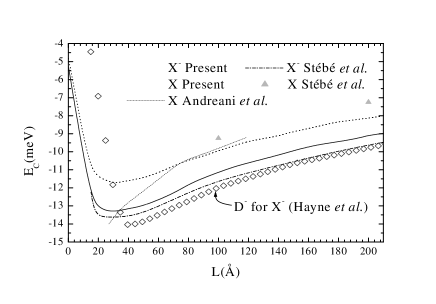
FIG. 1.: The correlation energy of the exciton and the negative charged exciton vs. the quantum well width.

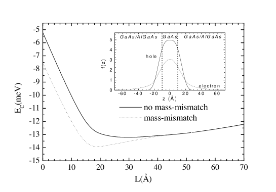
FIG. 2.: The correlation energy of the negative charged exciton vs. the quantum well width, for the case of constant masses in the well and in the barrier, and for the the case of different electron and hole masses in the well and in the barrier of a GaAs/Al_0.3Ga_0.7As quantum well. In the inset the wave function for both the electron and the hole are shown.

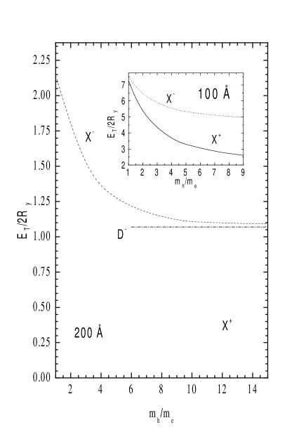
FIG. 3.: The total energy of the negative charged exciton and the positive charged exciton vs. $m_{h}/m_{e}$ for a 200 Å wide quantum well and for a quantum well of width 100 Å (inset). The total energy of a D^- in the same quantum well is given by the dash-dotted line for comparison.

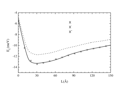
FIG. 4.: The correlation energy of the negatively charged exciton (symbols) and the one of the positively charged exciton (solid curve) vs. the well width. The correlation energy of the exciton (dotted curve) is given as reference.

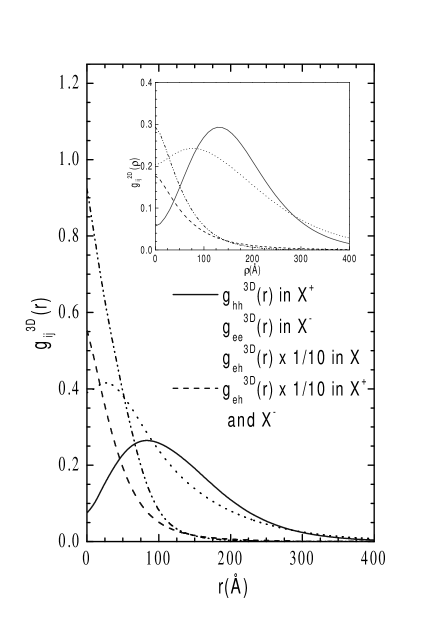
FIG. 5.: 3D pair correlation function for different pairs of particles in X^- and in X⁺ vs. the distance between the particles. In the inset the 2D pair correlation function is shown. The curve convention is the same in the two plots.

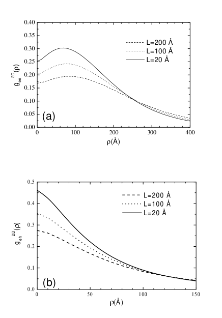
FIG. 6.: The pair correlation function for the electron-electron (a) and electron-hole (b) in X^- for different quantum well widths .

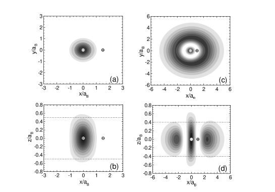
FIG. 7.: Contour maps of the conditional probability for the X^- in a quantum well of width 100Å$\approx$ a_B. The fixed particles are indicated by symbols (circle with a cross for the hole and circle with a minus sign for the electron). The dotted lines indicate the quantum well boundaries.

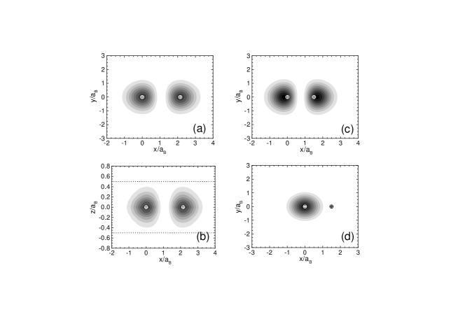
FIG. 8.: Contour maps of the conditional probability for the X⁺ in a quantum well of width 100 Å$\approx$a_B. The fixed particles are indicated by symbols (circle with a cross for the hole and circle with a minus for the electron). The dotted lines indicate the quantum well boundaries.

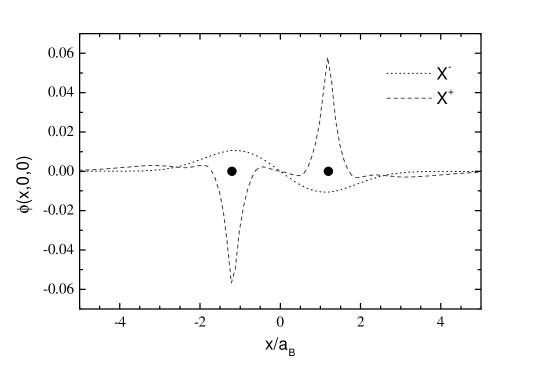
FIG. 9.: The wavefunction of the hole in X^- when the two electrons are fixed (dotted curve) and of the electron in X⁺ when the two holes are fixed (dashed curve) along the direction [1,0,0]. The two solid dots indicate the two equally charged fixed particles.

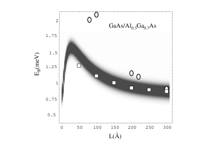
FIG. 10.: The theoretical (shaded curve) and experimental (open circles) binding energies of the negatively charged exciton in a GaAs/AlGaAs quantum well vs. the well width. The theoretical results of the quantum Monte Carlo calculation of Ref.22 are shown by the open squares.

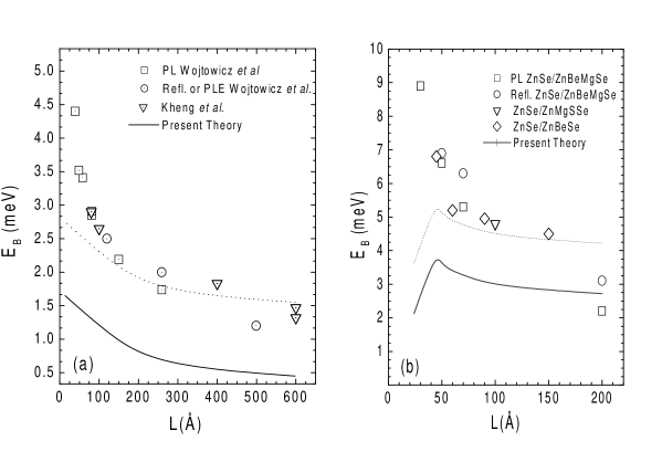
FIG. 11.: The binding energy of the negative charged exciton vs. the quantum well width for the charged exciton for CdTe-based structures (a) and for ZnSe-based structures (b). The experimental data are taken from Refs. 2,24, for the CdTe-based structures, and from Ref. 25 for the ZnSe-based structures. Our theoretical results are given by the solid curve. The dotted curve is our result shifted by a constant.

REFERENCES

- [1] Electronic address: riva@uia.ua.ac.be.
- [2] Electronic address: peeters@uia.ua.ac.be.
- [3] on leave of absence from the Institute of nuclear physics of the Hungarian Academy of Sciences, Debrecen, Hungary.
- [4] M. A. Lampert, Phys. Rev. Lett. 1, 450 (1958).
- [5] K. Kheng, R. T. Cox, Y. Merle d’Aubigne, F. Bassani, K. Saminadayar, and S. Tatarenko, Phys. Rev. Lett. 71, 1752 (1993); K. Kheng, K. Saminadayar, and N. Magnea, J. Cryst. Growth 184/185, 849 (1998).
- [6] G. Finkelstein, H. Shtrikman, and I. Bar-Joseph, Phys. Rev. B 53, R1709 (1996); G. Finkelstein, H. Shtrikman, and I. Bar-Joseph, Phys. Rev. B 53, 12593 (1996).
- [7] A. J. Shields, J. L. Osborne, D. M. Whittaker, M. Y. Simmons, M. Pepper, and D. A. Ritchie, Phys. Rev. B 55, 1318 (1997); A. J. Shields, F. M. Bolton, M. Simmons, M. Pepper, and D. A. Ritchie, Phys. Rev. B 55, R1970 (1997).
- [8] G. Munschy and B. Stébé, Phys. Stat. Sol. (b) 64, 213 (1974).
- [9] B. Stébé and A. Aniane, Superlatt. Microstruct. 5, 545 (1989).
- [10] J. R. Chapman, N. F. Johnson, and V. N. Nicopoulos, Phys. Rev. B 55, R10221 (1997).
- [11] D. M. Whittaker and A. J. Shields, Phys. Rev. B 56, 15185 (1997).
- [12] F. Dujardin, A. El Hassani, E. Feddi, and B. Stébé, Solid State Commun. 103, 515 (1997).
- [13] C. Riva, K. Varga, and F. M. Peeters, accepted for publication in Phys. Stat. Sol.(b) (proceedings OECS-6,Ascona, Switzerland, 1999).
- [14] B. Stébé, G. Munschy, L. Stanuffer, F. Dujardin, and J. Murat, Phys. Rev. B 56, 12454 (1997).
- [15] Y. Suzuki and K. Varga , Stochastic Variational Approach to Quantum-Mechanical Few-Body Problems (Springer, Berlin-Heidelberg, 1998).
- [16] G. Oelgart, M. Proctor, D. Martin, F. Morier-Genaud, and F.-K. Reinhart, B. Orschel, L. C. Andreani, and H. Rhan, Phys. Rev B 49, 10456 (1994).
- [17] L. C. Andreani and A. Pasquarello, Phys. Rev. B 42, 8928 (1990).
- [18] M. Hayne, C. L. Jones, R. Bogaerts, C. Riva, A. Usher, F. M. Peeters, F. Herlach, V.V. Moshchalkov, and M. Henini, Phys. Rev. B 59, 2927 (1999).
- [19] I. K. Marmorkos, V. A. Schweigert, and F. M. Peeters, Phys. Rev. B 55, 5056 (1997); C. Riva, V. A. Schweigert, and F. M. Peeters, Phys. Rev. B 57, 15392 (1998).
- [20] C. Riva, K. Varga, V. A. Schweigert, and F. M. Peeters, Phys. Stat. Sol. (b) 210, 689 (1998).
- [21] B. H. Brasden and C. J. Joachim, Physics of Atoms and Molecules (Longman Scientific & Technical, Hong Kong, 1987), p.147.
- [22] R. Kaur, A. J. Shields, J. L. Osborne, M. Y. Simmons, D. A. Ritchie, and M. Pepper, accepted for publication in Phys. Stat. Sol. (b) (proceedings OECS-6,Ascona, Switzerland, 1999).
- [23] A. J. Shields, M. Pepper, D. A. Ritchie, M. Y. Simmons, and G. A. C. Jones, Phys. Rev. B 51, 18049 (1995).
- [24] Z. C. Yan, E. Goovaerts, C. Van Hoof, A. Bouwen, and G. Borghs, Phys. Rev. B. 52, 5907 (1995).
- [25] T. Tsuchiya and S. Katayama, Proceeding of the 24th International Conference on The Physics of Semiconductors, Jerusalem, Israel, (1998), CD-rom.
- [26] O. Mayrock, H-J Wünsche, F. Henneberger, C. Riva, V. Schweigert, and F. M. Peeters, Phys. Rev. B 60, 5582 (1999); W. Langbein and J. M. Havm, Phys. Rev. B 59, 15405 (1999).
- [27] T. Wojtowicz, M. Kutrowski, G. Karczewski, and J. Kossut, Acta Physica Polonica A 94, 199 (1998).
- [28] D. R. Yakovlev, G. V. Astakhov, V. P. Kochereshko, A. Keller, W. Ossau and G. Landwehr, Proceeding of 7th Int. Symp. ” Nanostructures: Physics and Technology”, St. Petersburg, Russia, (1999), pp. 393.
- [29] A. De Nardis, V. Pellegrini, R. Colombelli, F. Beltrami, I. N. Kritvorotov, and K. K. Bajaj, submitted to Phys. Rev. B.
- [30] J. M. Shi, F. M. Peeters, G. A. Farias, J. A. K. Freire, G. Q. Hai, J. T. Devreese, S. Bednarek, and J. Adamowski, Phys. Rev. B 57, 3900 (1998).
- [31] J. M. Shi, F. M. Peeters, J. T. Devreese, Y. Imanaka, and N. Miura, Phys. Rev. B 52, 17205 (1995).