Ground state spin and Coulomb blockade peak motion in chaotic quantum dots

Abstract

We investigate experimentally and theoretically the behavior of Coulomb blockade (CB) peaks in a magnetic field that couples principally to the ground-state spin (rather than the orbital moment) of a chaotic quantum dot. In the first part, we discuss numerically observed features in the magnetic field dependence of CB peak and spacings that unambiguously identify changes in spin $S$ of each ground state for successive numbers of electrons on the dot, $N$. We next evaluate the probability that the ground state of the dot has a particular spin $S$, as a function of the exchange strength, $J$, and external magnetic field, $B$. In the second part, we describe recent experiments on gate-defined GaAs quantum dots in which Coulomb peak motion and spacing are measured as a function of in-plane magnetic field, allowing changes in spin between $N$ and $N+1$ electron ground states to be inferred.

I Introduction

In the absence of interactions, electrons populate the orbital states of a quantum dot or metallic grain in an alternating sequence of spin-up and spin-down states, in accordance with the Pauli picture. In this case, the total spin of the dot is either zero, when the number of electrons $N$ is even, or one half at odd $N$. No higher spin states appear. It is well known that in the presence of interactions, this simple scheme can be violated. Such deviations from simple even-odd filling may appear as Hund’s rules in atomic physics, or be as extreme as complete spin polarization leading to ferromagnetism by the mechanism of the Stoner instability.

By measuring electron transport through a weakly coupled quantum dot at low temperature and bias voltage (compared to the quantum level spacing) one can effectively study differences in ground state (GS) properties of the dot at successive electron number, providing a means of investigating the actual filling scheme [1]. A standard experimental approach [1] is to measure conduction through the dot via two tunneling leads as a function of a voltage, $V_{g}$, applied between the dot and a third electrically isolated electrode, known as a gate. Because the dot GS energy, $E_{N}$, at a fixed electron number is influenced by $V_{g}$, the gate can be used to set the number of electrons on the dot. The fact that a large Coulomb energy is needed to add a single electron to the dot typically suppresses conduction through the dot in the tunneling regime, where whole charges must tunnel for conduction to occur. This effect is known as the Coulomb blockade (CB). However, at specific values of gate voltage, denoted $V_{g}^{(N)}$, where the condition $E_{N-1}(V_{g})=E_{N}(V_{g})$ is satisfied, conductance increases dramatically, clearly marking this degeneracy condition in an experimental trace. The position, $V_{g}^{(N)}$, of the $N^{th}$ peak in the conductance is proportional to $\mu_{N}=E_{N}(0)-E_{N-1}(0)$. Accordingly, the distance between successive peaks is $\Delta_{2}^{N}=\mu_{N}-\mu_{N-1}$. (We take the constant of proportionality converting gate voltage to dot energy to be unity for the theoretical discussion; experimentally, this constant can be readily measured, for instance, by comparing the influence of bias and gate voltages.)

In the last few years the GS spin of a variety of nanostructures, including metallic grains[2], semiconducting quantum dots [3, 4, 5, 6], and carbon nanotubes [7, 8], have been investigated using CB peak motion in a magnetic field. If one neglects the magnetic field coupling to the orbital degrees of freedom, one expects the field to manifest itself only through the Zeeman splitting, resulting in a shift of the GS energy by $g\mu_{B}SB$, where $\mu_{B}$ is the Bohr magneton and $S$ denotes the GS total spin. For 2D quantum dots, orbital coupling can be strongly suppressed—though not eliminated entirely—by orienting the field strictly in the 2D plane. This is the experimental approach that will be described in Section III of this paper. On the other hand, for ultrasmall grains and nanotubes, it is reasonable to ignore orbital coupling for any field direction since for practical magnetic fields the total flux cutting the structure is much less than the quantum of flux.

For semiconducting quantum dots [3, 4, 5, 6] the Zeeman splitting for $S=1/2$ becomes comparable to the mean single electron level spacing

$$\delta_{1}=\langle s_{i}\rangle;\ \ \ s_{i}=\varepsilon_{i}-\varepsilon_{i+1},$$ (1)

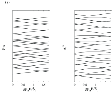
(here $\varepsilon_{i}$ denotes the orbital energy of the one-electron orbital state $i$, and $\langle\ldots\rangle$ stands for an average over different levels) at $B\sim 1\,T$ for the GaAs dots is Refs.  [4, 6] and $B\sim 10\,T$ for the Si dot in Ref. [3]. At lower fields, the splitting seldom exceeds $s_{i}$, and one might expect a simple even/odd Pauli picture. In this case, CB peak positions would move with $B$ as consecutive pairs, creating a pattern of alternating downward and upward moving peaks, as seen in Fig. 1a. The trajectories of the pair of peaks would form straight lines with the same slope of $g\mu_{b}/2$. The peak spacings, $\Delta^{N}_{2}$, will have a similar pattern with slopes of $g\mu_{b}$. Spin-orbit interaction can lead to fluctuations in the $g$ factor, resulting in fluctuations in the slopes of the lines, [9, 10], but will not change the pattern of downward and upward moving peaks. Once $g\mu_{b}B$ exceeds a particular spacing $s_{i}$, the peaks should cross.

Experimentally, the Pauli picture appears to work well for metallic grains [2], while for carbon nanotubes the situation is less clear: one published experiment finds simple even/odd filling [7], and one finds a more complicated scheme [8]. For multielectron semiconducting dots [3, 4, 6] the data are somewhat confusing, but appear to disagree with the simple even/odd filling scheme [3, 4, 6, 11], presumably as a result of electron-electron interactions. In symmetric, few-electron vertical dots [12] one may again recover relatively simple behavior for the first few electrons, with a well-understood appearance of Hund’s rules. These conclusions are based on experiments where orbital magnetism dominates spin. However, for few electrons (i.e., $N\lesssim 10$) the filling scheme can be readily interpreted, allowing the full spin structure to be mapped out as a function of $N$ and $B$ [12].

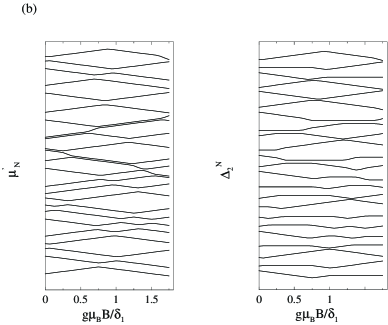
Figure 1 shows CB peak motion and spacing as a function of magnetic field (coupling only to spin) for both a noninteracting electron model and an interacting electron model presented in detail in Section II. The behavior of this model appears more similar to the experimentally observed behavior in semiconducting quantum dots (see Fig. 6). In some cases peak positions ($\mu_{N}$) move as function of the magnetic field in bunches of two in the same direction and with the same slope, while their corresponding spacings ($\Delta_{2}^{N}$) do not change as function of the magnetic field. Moreover, not every change in the direction of the motion of a peak can be explained as a crossing of two orbital levels. Thus, a description of the system beyond the Pauli picture is needed.

We will present a theory that goes beyond the simple Pauli picture and explains the puzzling features of the magnetic field dependence of the conductance peaks positions as a result of spontaneous spin polarization of the electrons in the dot [14]. The possibility of spontaneous magnetization in quantum dots has been considered in different contexts [14, 15, 16, 17, 18, 19, 20]. For instance, it has also been suggested as an explanation [16] for the absence of a bimodal distribution in the conductance peak spacings [21]. Such a magnetization was also predicted to lead to kinks in the parametric motion of the peaks, (e.g., due to orbital effects of a perpendicular magnetic field) [19].

FIG. 1.: Typical conductance dependence on the gate voltage and magnetic field, $B$, with and without exchange interaction: (a) $J=0$, (b) $J=0.1\delta_{1}$. $\mu^{\prime}_{N}$ is determined as $\mu^{\prime}_{N}=\mu_{N}-e^{2}/C$ and taken in arbitrary units. $\Delta_{2}^{N}$ for each $N$ is shifted arbitrarly by $N\times$constant to avoid overlapping.

II Theory

We begin the theoretical discussion by reviewing the considerations determining the general form of the Hamiltonian describing the properties of a chaotic dot in the metallic regime. A more complete description may be found in Ref. [14]. The single electron spectrum $\varepsilon_{i}$ is characterized by the mean level spacing $\delta_{1}$ and the Thouless energy $E_{T}\approx\hbar/t_{erg}$, where $t_{erg}$ is the time it takes for a classical electron to cover the energy shell in the single-particle phase space. For diffusive and ballistic systems $t_{erg}$ equals to $L^{2}/D$ and $L/v_{F}$ respectively, where $v_{F}$ is the electronic Fermi velocity, $L$ is the system size, and $D$ is the diffusion coefficient. The dimensionless conductance, $g_{T}=E_{T}/\delta_{1}$, in the metallic regime is large, i.e., $g_{T}\gg 1$. In this regime the statistics of the single electron spectrum on scales smaller than $E_{T}$ are well described by random matrix theory (RMT) [22], which gives a quantitative description of the phenomenon of level repulsion. For an ensemble of $M\times M$ matrices ($M\rightarrow\infty$) with random and independent elements, the probability density of a realization of the spectrum $\varepsilon_{i}$ is given by[22]:

$$P(\varepsilon_{i})\propto\exp\left[\frac{\beta}{2}\sum_{i\neq j}\ln\left(\frac{|\varepsilon_{i}-\varepsilon_{j}|}{\delta_{1}}\right)\right],$$ (2)

where $\beta$ is equal to $1$, $2$ or $4$ for the orthogonal, unitary and symplectic ensembles respectively. The orthogonal (unitary) RM ensemble corresponds to weakly disordered dots with preserved (violated) time reversal symmetry and negligible spin-orbit. We assume that the dot is small enough for the spin-orbit interaction to be negligible and thus avoid discussion of the symplectic ensemble ($\beta=4$) [13].

The second step is to consider effects of electron-electron interactions. For the simplest case of short-range interactions, we write

$$H_{int}(\vec{r})=\lambda\delta_{1}V\delta(\vec{r}),$$ (3)

where $V\propto L^{d}$ is the volume of the dot (in $d$ dimensions) and $\lambda$ is a dimensionless coupling constant characterizing the strength of the interaction. Matrix elements of this interaction, in the basis of eigenstates $\varphi_{i}(\vec{r})$ of the noninteracting Hamiltonian, are given by

$$M^{ij}_{kl}=\lambda\delta_{1}V\int d\vec{r}\varphi_{i}^{\ast}(\vec{r})\varphi_{j}^{\ast}(\vec{r})\varphi_{k}(\vec{r})\varphi_{l}(\vec{r}).$$ (4)

It is important to note that the statistical properties of the interaction matrix elements $M^{ij}_{kl}$ are completely determined by the statistical properties of the single electron eigenstates $\varphi_{i}(\vec{r})$ and cannot be chosen in an arbitrary fashion as in the random interaction model[20]. In fact, in the limit $g_{T}\to\infty$ the diagonal matrix elements ($i,j,k,l$ pairwise equal) are self-averaged by the space integration, Eq. (4), and thus show no level-to-level or sample-to-sample fluctuations[14]. In the same limit the off-diagonal matrix elements Eq. (3) turn out to be negligable.

Using the statistical properties of the interaction matrix elements it turns out that a large class of disordered metallic dots can, under very general conditions, be described by a remarkably simple Hamiltonian with only three coupling constants, which do not fluctuate. In the limit of large $g_{T}$, the interaction part of the Hamiltonian corresponds to

$$H_{int}=E_{c}\hat{N}^{2}-J(\vec{S})^{2}+\lambda_{BCS}\hat{T}^{\dagger}\hat{T},$$ (5)

(terms linear in $\hat{N}$ are allowed, but they can be included into the one-particle part of the Hamiltonian) where $\hat{N}$ is the number operator, $\vec{S}$ is the spin operator and $\hat{T}=\sum_{i}c_{i\uparrow}c_{i\downarrow}$ ($c_{i\uparrow}$ annihilates an electron in the $i^{th}$ single electron orbital with spin $\uparrow$). In the simple model with short-range interaction and preserved time reversal ($\beta=1$) the above coupling constants have the following form:

$$E_{c}=\frac{1}{2}\lambda\delta_{1};\quad J=2\lambda\delta_{1};\quad\lambda_{BCS}=\lambda\delta_{1}.$$ (6)

If time invariance is broken ($\beta=2$), $\lambda_{BCS}=0$ since the operator $\hat{T}$ is incompatible with the symmetry. Note that the interaction Hamiltonian Eq. (3) represents a particular model, and the expressions for the coupling constants Eq. (6) are valid only for this model. At the same time, the effective interaction Hamiltonian, Eq. (5), is more robust and depends only on the symmetries of the problem (for instance, on the absence of the spin-orbit scattering) and on the condition $g_{T}\gg 1$.

The first two terms in Eq. (5) represent the dependence of the energy of the dot on the total number of the electrons and on the total spin respectively. They commute with each other and with the single-particle part of the Hamiltonian. Therefore, all states of the grain can be classified by $N$ and $S$. The term proportional to $\lambda_{BCS}$ appears only in the orthogonal case $(\beta=1)$. Provided that $\lambda_{BCS}<0$ this term leads to the superconducting instability. Superconducting correlations are suppressed by the magnetic field, and thus do not exist for $\beta=2$.

Thus, the general form of the Hamiltonian describing electrons in a chaotic dot which is not superconducting is given by

$$H=\sum_{i}\varepsilon_{i}n_{i}+E_{c}N^{2}-JS(S+1)+g\mu_{b}SB.$$ (7)

Note that the only random component of the problem is the single-particle spectrum $\varepsilon_{i}$, while the exchange $J$ and charging energy $E_{c}$ do not fluctuate. It should be realized, though, that Eqs. (5,7) become exact only in the limit $g_{T}\to\infty$. The corrections to Eqs. (5,7), which appear at finite $g_{T}$ are sometimes important. However, if $g_{T}\gg 1$, these corrections do not bring essentially new physics to the problem of spin magnetization.

The conductance is calculated using the many-particle energies $E_{N}$ and wave functions obtained numerically for GOE and GUE random matrix realizations. An example of the peak positions and peak spacing evolution as functions of the magnetic field for a particular GOE realization is presented in Fig. 1 for (a) $J=0$ and (b) $J=0.1\delta_{1}$. For both cases we present $\mu_{N}^{\prime}=\mu_{N}-E_{c}$. The noninteracting case, Fig. 1a, shows all the previously described features of the Pauli behavior. Once a weak exchange interaction is included the behavior changes qualitatively, not just at high field, but also in the vicinity of $B=0$. In particular, peak positions are not always paired, resulting in occasional field-independent peak spacings. This occurs when two consecutive orbitals are first filled with down spin electrons and only later they acquire up electrons. Generally the enhancement of the spin of the dot by $S$ will be accompanied by a $2S$ bunch peaks moving with the same slope. If the peak spacing $\Delta_{2}^{N}$ is plotted, two sets of $2S-1$ flat curves sandwiching a sloped one will appear. Changes to the crossing also attributed to a sudden change of the GS spin which is not associated with a single electron orbital crossing.

As illustrated above, the appearance of higher spin clearly manifests itself in the peak position and peak spacing trajectories. Using Eq.(7) one can predict the frequency of spontaneous magnetization appearances. For weak exchange, $J\ll\delta_{1}$, the probability that the dot GS has a spin $S$ is determined by the probability of finding $2S$ orbitals so close to each other that the gain in exchange energy (due to the polarization) overwhelms the loss in the kinetic energy (due to single rather than double occupations of the orbitals).

Thus the probability for a certain value of ground state magnetization $S$ boils down to the question of the probability of finding $2S$ close single electron levels. That probability may be estimated using random matrix theory, as we now present.

The probability of finding a set of single electron orbital at energies $\varepsilon_{i}$ is given by Eq. (2). Thus as long as

$$\varepsilon_{i+2S}-\varepsilon_{i}<JS(S+1)+g\mu_{B}BS,$$ (8)

a ground state spin of at least $S$ will appear. Taking into account the probability of Eq. (2), it is possible to write the probability of obtaining a ground state spin $S$ as a function of the linear combination:

$$X={{J}\over{\delta_{1}}}+{{g\mu_{B}B}\over{\lfloor S+{{3}\over{2}}\rfloor\delta_{1}}},$$ (9)

resulting in the following probability

$$P_{J,B}(S)=C^{\beta}_{S}X^{(\beta S+1)(2S-1)}(1-K_{S}^{\beta}X^{2}),$$ (10)

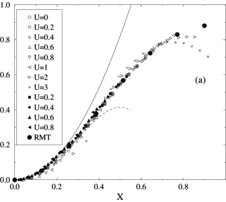
The coefficients $C_{S}^{\beta}$ and $K_{S}^{\beta}$ depend on both $\beta$ and $S$. Their values for $S=1,3/2$ are presented in table I.

	$\beta=1$		$\beta=2$
	$S=1$	$S=3/2$	$S=1$	$S=3/2$
$C$	$\pi^{2}/3$	$9\pi^{4}/50$	$8\pi^{2}/9$	$81\pi^{6}/400$
$K$	$\pi^{2}/5$	$18\pi^{2}/49$	$8\pi^{2}/25$	$792\pi^{2}/1225$

TABLE I.: The factors $C_{S}^{\beta}$ and $K_{S}^{\beta}$ appearing in Eq. (10).

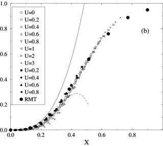
Thus the RMT model presents a striking conclusion. The influence of exchange interactions and externally applied magnetic field on the ground state magnetization of a quantum dot may be summed up in a single parameter scaling function, where the scaling parameter is a simple linear combination of $J$ and $B$. As has been shown from numerical simulations[23], the scaling holds for larger values of $X$ than expected from the first and second term perturbative analysis presented in Eq. (10).

One may wonder how well does the above picture hold for systems for which real correlation between the electron exist, and the dimensionless conductance is not too large. A canonical example for such systems is the Hubbard model:

$$H=\sum_{i,\sigma}\epsilon_{i}a_{i,\sigma}^{{\dagger}}a_{i,\sigma}-t\sum_{<i,j>,\sigma}(a_{i,\sigma}^{{\dagger}}a_{j,\sigma}+h.c)$$ (11)

$$+U\sum_{i}{a_{i,\uparrow}^{{\dagger}}a_{i,\uparrow}a_{i,\downarrow}^{{\dagger}}a_{i,\downarrow}}+g\mu_{B}SB$$ (12)

where $<i,j>$ denotes nearest neighbor lattice site, $a_{i,\sigma}^{{\dagger}}$ is an creation operator of an electron at site $i$ with spin $\sigma$, $\epsilon_{i}$ is the site energy, chosen randomly between $-W/2$ and $W/2$ with uniform probability, and $U$ is the interaction constant.

The Hilbert space is large even for relatively small systems. For example for a $4\times 4$ lattice with $6$ electrons for the $S=0$ sector has the size of $313600$. Using the Lanczos method we obtain the many-particle eigenvalues $E_{N}(S)$ as function of the ground state in each spin sector $S$ for different values of interaction $U$. The disorder was chosen as $W=8t$, which corresponds to the metallic regime, although the value of the dimensionless conductance is quite low $g_{T}\sim O(1)$.

FIG. 2.: Probabilities of $S=1$ for $J=0.1\delta_{1}$ as functions of the magnetic field $B$ for (a) the GOE and (b) GUE cases. The small symbols represent numerical results for the Hubbard model, the large filled symbols represent numerical results for the RMT model, while the curves (solid - first order, dashed - second order) represent Eq. (10).

We calculated the probability for the appearance of a specific value of GS spin $S$ for different values of $U$ and magnetic field $B$. In order to use the scaling parameter $X$ we need to deduce the appropriate value of $J$ for each value of $U$. This has been done by fitting the dependence of the average lowest energy in a given spin sector $\langle E(S)\rangle$ to

$$\langle E(S)\rangle=\delta_{1}s^{2}-JS(S+1).$$ (13)

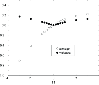
The distribution $P_{J(U),B}(S)$ based on numerical results for $1000$ different realizations of the Hubbard model, for different values of $U$ and $B$ for $\beta=1$ and $\beta=2$ is presented in Fig. 2. Although some deviations do appear, especially for the higher values of $U$, one can see that the overall form of the scaling function holds remarkably well. Thus, though the Hamiltonian in Eq. (7) is obtained under the conditions of large $g_{T}$ and no correlations in the system, it nonetheless appears to capture much of the physics even for a moderate $g_{T}$ and in the presence of electron-electron correlations. The reason for this is that although neither $J$ nor $E_{c}$ is constant once $g_{T}\sim 1$, their fluctuations remain small relative to their average, as is demonstrated in Fig. 3.

FIG. 3.: The exchange parameter $J$ as functions $U$ for a $4\times 4$ Hubbard model with 6 electrons.

III Experiment

In this section we describe recent experimental measurements of GS spin for a gate-defined GaAs quantum dot containing roughly 400 electrons. As discussed in the Introduction, the dot is coupled to electron reservoirs via tunnelling leads (i.e., $g<2e^{2}/h$ for both leads) so transport is dominated by CB effects. Measurements were carried out at sufficiently low temperature and bias that the differences in GS energies between dots with $N+1$ and $N$ electrons should be extractable from CB peak positions, $V_{g}^{(N)}$.

The dot is formed at the interface of a GaAs/AlGaAs heterostructure ($90\,nm$ below the wafer surface) by electrostatic depletion using surface gates. A Si delta doping region is located $40\,nm$ above the heterointerface. The two-dimensional electron gas (2DEG) has density $\sim 2.0\times 10^{11}\,cm^{-2}$ and bulk mobility $\sim 1.4\times 10^{5}\,cm^{2}/Vs$, yielding a transport mean free path $\sim 1.5\,\mu m$. The small dot area, $A\sim 0.25\,\mu m^{2}$, makes transport predominantly ballistic within the device. Characteristic energy scales for the measured device include the mean level spacing, $\Delta=2\pi\hbar^{2}/m^{*}A\sim 30\,\mu eV$, the charging energy, $E_{C}\sim 400\mu eV$, and the Thouless energy $E_{th}=\hbar v_{F}A^{-1/2}\sim 340\mu eV$. Measurements were carried out in a dilution refrigerator with a mixing chamber temperature of $25\,mK$ using standard ac lock-in techniques with a source-drain bias voltage of $2\,\mu eV$. A base electron temperature of $T_{e}\sim 50\,mK$ was determined from CB peak widths.

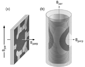
To allow the magnetic field to couple predominantly to spin, the sample was oriented with the plane of the electron gas along the axis of the primary solenoid, aligned manually to within 0.5 degrees. In addition, a small pair of coils attached to the vacuum can of the fridge, oriented perpendicular to the plane of the sample (see Fig. 4), was used to null out any perpendicular field from misalignment as well as to explicitly break time-reversal symmetry. Both primary and trimming coils were under computer control, allowing sweeps of strictly parallel field by trimming out any perpendicular component for any applied parallel field. (We estimate the uncertainty in $B_{\perp}$ to be less than $\phi_{o}/4$ through the dot at $B_{\parallel}=5\,T$.) Despite this precise field trimming capability, similar measurements [6] in larger dots, fabricated on the same wafer, indicate orbital coupling due to the strictly parallel field for $B_{\parallel}\gtrsim 0.5T$ (evident, for instance, from the disappearance of the weak localization feature at $B_{\perp}=0$ at higher $B_{\parallel}$). The origin of this surprising coupling—which makes interpretation of our high-field data difficult—is still under investigation.

FIG. 4.: a) Schematic diagram of a gate-defined quantum dot, indicating the orientations of $B_{\parallel}$ and $B_{\perp}$ relative to the planar quantum dot. (Orientation of $B_{\parallel}$ within the plane is not accurately depicted and has not been investigated.) b) Diagram showing placement of superconducting coils used to generate $B_{\perp}$ on vacuum can, inside primary solenoid used to generate $B_{\parallel}$.

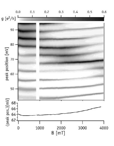
Conductance measurements across ten consecutive Coulomb blockade peaks, measured as a function of $V_{g}$ and $B_{\parallel}$ (i.e., strictly $B_{\parallel}$, properly trimmed), are shown in Fig. 5a. More positive gate voltage corresponds to higher energy, and can be calibrated from the CB “diamonds” using high source-drain bias measurements [1]. All data are taken with $B_{\perp}=20mT$ in order to ensure that time-reversal symmetry is broken, which changes the statistics of dot wave functions.

In addition to the individual motions of each peak, there is a diamagnetic shift of all peaks (see Fig. 5b), presumably due to the effect of the parallel field on the effective well confinement potential. The slight paramagnetic shift visible at low field, $(B_{\parallel}<0.2T)$, is not understood at present. In the following analysis of data, the common curve (in Fig. 5b) has been subtracted from each peak position.

FIG. 5.: a) Nine consecutive Coulomb blockade peaks measured as a function of gate voltage $V_{g}$ and parallel field $B$. Conductance is shown in grayscale, with black indicating high conductance and white low conductance. The field shown on the bottom axis is the field strictly parallel to the heterointerface; perpendicular field is held constant at $20mT$ as discussed in the text. Note that conductance in the valleys is low but not zero, due to strong tunnelling in the leads. b) Average peak position of the peaks in a), showing a diamagnetic shift to higher energies common to all peaks. This average is subtracted from all peak positions before further analysis.

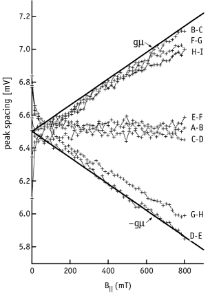
Peak positions and peak spacings extracted from the peaks in Fig. 5 are shown in Fig. 6. The slope of peak positions as a function of $B_{\parallel}$ is consistent with a Zeeman energy term $E_{S}=\pm\frac{1}{2}g\mu_{B}B$, using the $g$-factor for bulk $GaAs$, $|g|=0.44$. As discussed in the Introduction, alternating slopes for consecutive peaks would indicate an alternating $0,\frac{1}{2},0,\frac{1}{2}...$ GS spin structure. Our data, on the other hand, shows three consecutive pairs of peaks moving with the same slope, suggesting the presence of higher spin states. Proposed values for the eight consecutive GS spin states shown here are included in Fig. 6a. We emphasize, however, that these are only plausible values for the spin; it is not possible to determine unambiguously the absolute magnitude of GS spin from measurements of peak position, which reflect changes in spin from the N to N+1 ground states. The values shown in Fig. 6a minimize the ground state spin for the system.

FIG. 6.: a) Peak positions (with average motion subtracted) as a function of parallel field for the nine peaks shown in Fig. 5a. Straight lines indicate expected peak motion for spin-$\frac{1}{2}$ transitions using the $g$ factor for bulk $GaAs$, $|g|=0.44$. Positive slopes indicate transitions to lower spin states; negative slopes indicate transitions to higher spin states. Numbers indicate a possible ground-state spin structure for ten consecutive ground states. Peak position data are offset for clarity. b) Peak spacings for the position data shown in a), offset for clarity. Solid lines indicate expected motion of peak spacing for spin-$\frac{1}{2}$ transitions, using $|g|=0.44$

FIG. 7.: Peak spacings from Fig. 6b, offset to align spacings at $B_{\parallel}=0$. Slopes cluster in three branches, interpreted as a change from decreasing to increasing spin transitions (positive slope), two consecutive spin transitions in the same direction (zero slope), and a change from increasing to decreasing spin transitions (negative slope). Solid lines indicate expected motion of peak spacing for spin-$\frac{1}{2}$ transitions, using $|g|=0.44$, with no adjustable parameters.

FIG. 8.: Peak spacings from Fig. 6b, shown over an extended range of parallel field, up to $B_{\parallel}=4T$. Slopes tend to change abruptly between linear segments, with rounding between the segments possibly providing a measure of spin-orbit or other spin-mixing interaction.

FIG. 9.: Peak spacings for five peaks at low parallel fields, measured after reducing the transmission of the point contacts to allow only weak tunnelling between the dot and the leads. For the four consecutive spacings shown, all have slopes considerably less than $g\mu$.

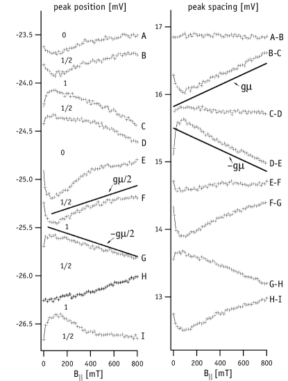
In the proposed spin labelling scheme, three out of the five even-$N$ states have $S=1$, i.e., $P(S=1)\sim 0.6$. This fraction of $S=1$ relative to the number of $S=0$ states is well beyond the expected value given reasonable estimates of $J$ for $GaAs$ dots. Of course, with only five spin states considered, statistics are quite poor. Further experiments are needed to see if this discrepancy is significant.

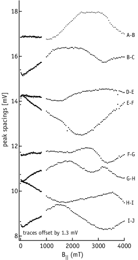
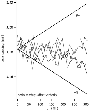
Figure 7 shows that peak spacings clearly separate into three branches, a top branch with slope roughly $g\mu$ (corresponding to a GS spin decrement followed by an increment) a bottom branch with slope roughly $-g\mu$ (corresponding to a GS spin increment followed by a decrement) and a middle branch with slope near zero (corresponding to two consecutive increments or decrements). The existence of the middle branch is the signature of higher GS spins. The good agreement between the slopes of the upper and lower branches and the expected slopes of $g\mu$, as well as the absence of a range of intermediate slopes suggest that the peak spacing reflects spin rather than orbital coupling. At higher fields, the directions of peak motion change, often abruptly and from one straight segment to another, as seen in Fig. 8. This behavior is qualitatively similar to the numerical data in Fig. 1b. The rounding of straight segments where the slope changes presumably results from spin-orbit interaction which mixes spins, and may provide a direct measure of spin-orbit interactions in dots. It is interesting to note that the peaks analyzed in Figs. 6 through 8 were measured in a regime of high tunneling conduction in the leads. This can be seen by noting the grayscale of Fig. 5. When the dot is more pinched off from the reservoirs, so that the CB peaks have a height of $0.1\;e^{2}/h$ or less, peak motion is more difficult to interpret, and does not seem to follow the clear patterns illustrated, for instance, in Fig. 8. As seen in Fig. 9, peak spacings for four consecutive weak-tunneling peaks at do not move with slopes of $g\mu$ at low $B_{\parallel}$. Though the data are noisier in this configuration, it is clear that the slopes are in all cases less than $g\mu$. We do not have an explanation for the different behavior depending on if the dot is more closed off or nearly open.

IV Discussion

In conclusion, we have shown that a relatively weak exchange interaction qualitatively explains the deviations from the Pauli picture seen in recent experiments [3, 4, 6]. We calculate the probability that different values of spin appear as a function of exchange interaction and magnetic field coupling to the spin. The strength of the exchange interaction, $J$, and the effective $g$ factor are the only adjustable parameters that determine the probabilities for a GS of the dot to have any given spin at any given magnetic field for both GOE and GUE cases. In particular we predict that these probabilities will follow a one-parameter scaling law over a wide range of magnetic fields and exchange interaction strengths. We also report preliminary experiments to investigate the exchange effects in the ground state spin of quantum dots. The signature of interaction effects is the appearance of higher-spin ground states, which show up in the experimental data as peak spacing traces that have zero slope as a function of parallel magnetic field. Such features are indeed observed, as seen for instance in Fig. 8. Further experiments are needed to obtain sufficient statistics to quantitatively test the predictions of theory.

Support from ARO-MURI DAAG55-98-1-0270 at Princeton and Harvard is gratefully acknowledged. We thank B. I. Halperin and L. P. Rokhinson for many useful discussions, and S. M. Cronenwett for assistance with experiments and analysis. The measured device was fabricated by S. R. Patel on material grown by C. I. Duruöz in the lab of J. S. Harris, Jr. at Stanford University. JAF acknowledges support as a DoD Fellow.

REFERENCES

- [1] M. A. Kastner, Rev. Mod. Phys. 64, 849 (1992); R. C. Ashoori, Nature 379, 413 (1996); Kouwenhoven et al., in Mesoscopic Electron Transport, Ed. by L. L. Sohn, L. P. Kouwenhoven, and G. Schön (Kluwer, Dordecht, 1997).
- [2] D. C. Ralph, C. T. Black and M. Tinkham, Phys. Rev. Lett. 74, 3241 (1995).
- [3] L. P. Rokhinson et al., cond-mat/0005262 (2000).
- [4] D. S. Duncan et al., Appl. Phys. Lett. 77, 2183 (2000).
- [5] J. A. Folk et al., cond-mat/0005066 (2000).
- [6] J. A. Folk et al., to be published.
- [7] D. H. Cobden et al., Phys. Rev. Lett. 81, 681 (1998).
- [8] S. J. Tans et al., Nature 393, 49 (1998).
- [9] K. A. Matveev, L. I. Glazman and A. I. Larkin, cond-mat/0001431
- [10] P. W. Brouwer, X. Waintal and B. I. Halperin, cond-mat/0002139
- [11] D. R. Stewart et al., Science 278, 1784 (1998).
- [12] S. Tarucha et al., Phys. Rev. Lett. 77, 3613 (1996).
- [13] B. I. Halperin, et. al, cond-mat/0010064 (2000).
- [14] I. L. Kurland, I. L. Aleiner and B. L. Altshuler, cond-mat/0004205.
- [15] A. V. Andreev and A. Kamenev, Phys. Rev. Lett. 81, 3199 (1998).
- [16] R. Berkovits, Phys. Rev. Lett. 81, 2128 (1998).
- [17] P.W. Brouwer, Y. Oreg and B.I. Halperin, Phys. Rev. B60, R13977 (1999).
- [18] E. Eisenberg and R. Berkovits, Phys. Rev. B 60, 15261 (1999).
- [19] H.U. Baranger, D. Ullmo and L.I. Glazman, Phys. Rev. B 61, R2425 (2000).
- [20] P. Jacquod and A. D. Stone, Phys. Rev. Lett. 84, 3938 (2000).
- [21] U. Sivan,et al., Phys. Rev. Lett. 77, 1123 (1996); F. Simmel,et al., Europhys. Lett. 38, 123 (1997); S.R. Patel,et al., Phys. Rev. Lett. 80, 4522 (1998); F. Simmel,et al., Phys. Rev. B 59, R10441 (2000) .
- [22] M. L. Mehta Random Matrices, (Academic Press, NY, 1991).
- [23] I. L. Kurland, R. Berkovits and B. L. Altshuler, cond-mat/0005424.