Anisotropic conductivity in superconducting NCCO

The pairing symmetry of electron-doped cuprate materials has been the subject of renewed interest in the last year. Previously existing experimental data were interpreted to be consistent with an s-wave order parameter [1]. In particular penetration depth measurements [2], Raman scattering [3], and tunneling data [4] were explained in this way. Surprisingly, however, recent microwave experiments [6, 7] and phase-sensitive tricrystal experiments [5] have provided evidence in favor of a d${}_{x^{2}-y^{2}}$-wave pairing symmetry.

In this report we examine the low temperature behaviour of the anisotropic conductivity in superconducting electron doped cuprates. Using a tilted film geometry, Pimenov et al. [12] have recently measured simultaneously $\sigma_{c}$ and $\sigma_{ab}$ ($c$-axis and in-plane conductivity) on Nd_2-xCe_xCuO₄ (NCCO) samples. By measuring the transmission through thin films as well as the transmission phase shift with an interferometer, both complex conductivities were determined in the submillimiter frequency range. Their results show a characteristic temperature dependence of $\sigma_{c}$ and $\sigma_{ab}$ in the superconducting state, varying both linearly with $T$ almost up to $T_{c}$. Fig. 1 shows an example of these experimental data [12] for a NCCO film with $T_{c}\approx 20$ K. Fits to the low temperature data are added to underline the linear $T$ dependence of both conductivities. In what follows we show how this linear $T$ dependence is consistent with a d${}_{x^{2}-y^{2}}$-wave order parameter under certain assumptions for the scattering rate ($\Gamma_{\bf k}$) and the c-axis hopping amplitude ($t_{\perp}({\bf k})$).

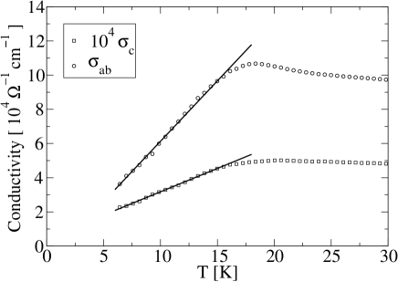
FIG. 1.: Experimental data for the real part of the c-axis ($\sigma_{c}$) and the in-plane conductivity ($\sigma_{ab}$) of a NCCO film with $T_{c}=20$ K at the frequency of $\nu=8$ cm^-1 (taken from Ref. [11]). The solid lines are linear fits to the low temperature part of the data.

For tetragonal cuprate compounds the interlayer c-axis hopping amplitude has the form [8]

$$t_{\perp}({\bf k})=-t_{\perp}\cos(k_{z}d)(\cos(k_{x}a)-\cos(k_{y}a))^{2},$$ (1)

where $k_{x}$, $k_{y}$ are the components of the in-plane momentum, $k_{z}$ the momentum along the $c$ axis and $a$ and $d$ are the corresponding lattice constants. From now on $a$ will serve as a length unit and is set to 1. The form of $t_{\perp}({\bf k})$ in Eq. (1) results from the hybridization between the bonding oxygen 2p and copper 4s orbitals in each CuO₂ plane which gives rise to the nodal structure of Eq. (1). A small deviation from the tetragonal structure leads to a finite value of $t_{\perp}({\bf k})$ also along the planar nodal directions. Similarly, isotropic impurity scattering is expected to effectively contribute to the $c$-axis transport. In this report we consider therefore the following extended form for $t_{\perp}({\bf k})$

$$t_{\perp}({\bf k})=-t_{\perp}[\cos(k_{z}d)(\cos(k_{x})-\cos(k_{y}))^{2}+c].$$ (2)

We are interested in the real part of the dc limit of the longitudinal conductivity both for the in-plane and the c-axis case. The conductivity, labeled by $\sigma_{\mu\mu}$, where $\mu$ is either $z$ or $x$, is given by:

$$\sigma_{\mu\mu}^{\prime}\equiv\hbox{Re}\ \sigma_{\mu\mu}=\lim_{\omega\rightarrow 0}\frac{\hbox{Im}\ D_{\mu\mu}(\omega+i0^{+})}{\hbar\omega}$$ (3)

where $D_{\mu\mu}(i\Omega)$ is the current-current correlation function

$$D_{\mu\mu}(i\Omega)=\lim_{{\bf q}\rightarrow{\bf 0}}\int_{0}^{\beta}e^{i\Omega\tau}\langle T_{\tau}\hat{\jmath}_{\mu}({\bf q},\tau)\hat{\jmath}_{\mu}({\bf-q},0)\rangle d\tau$$ (4)

with $\hat{\jmath}_{\mu}({\bf q},\tau)$ the paramagnetic current density operator. Note that the usual notation $\sigma_{c}$ corresponds to $\sigma_{zz}$ and $\sigma_{ab}$ to $\sigma_{xx}$. In Eq. (4) $\beta=1/T$, $T$ the temperature, $T_{\tau}$ the imaginary time ordering operator and $\Omega$ is a bosonic Matsubara frequency. For the purpose of comparing with experimental data in the submillimeter frequency range presented in Fig. 1 the zero frequency limit in Eq. (3) is appropriate.

Neglecting vertex corrections we rewrite $D_{\mu\mu}(i\Omega)$ as

$$D_{\mu\mu}(i\Omega)=\frac{1}{\beta N}\sum_{{\bf k},i\omega}j_{\mu}^{2}({\bf k})\hbox{Tr}\{G({\bf k},i\omega)G({\bf k},i\omega+i\Omega)\}.$$ (5)

$j_{x(z)}({\bf k})=e/\hbar(\partial\xi_{\bf k}/\partial k_{x(z)})$ is the current vertex function and $G({\bf k},i\omega)$ is the renormalized BCS Green’s function in Nambu space

$$G({\bf k},i\omega)=\frac{(i\tilde{\omega})\tau_{0}+\tilde{\xi}_{\bf k}\tau_{3}+\tilde{\Delta}_{\bf k}\tau_{1}}{(i\tilde{\omega})^{2}-\tilde{\xi}_{\bf k}^{2}-\tilde{\Delta}_{\bf k}^{2}}$$ (6)

where $\tilde{\omega}=\omega-\Sigma_{0}$, $\tilde{\xi}_{\bf k}=\xi_{\bf k}+\Sigma_{3}$ and $\tilde{\Delta}_{\bf k}=\Delta_{\bf k}+\Sigma_{1}$. $\xi_{\bf k}$ is the band dispersion measured with respect to the chemical potential, $\xi_{\bf k}=\epsilon_{\bf k}-\mu$, $\tau_{i}$ are the Pauli matrices, and $\Delta_{\bf k}$ is the superconducting gap that we take in a d${}_{x^{2}-y^{2}}$-wave form

$$\Delta_{\bf k}=\frac{\Delta_{0}}{2}(\cos(k_{x})-\cos(k_{y})).$$ (7)

$\Sigma_{i}$ are the components of the self energy matrix $\Sigma=\sum_{i=0}^{3}\Sigma_{i}\tau_{i}$ assumed to dominantly arise from impurity scattering in the low frequency and low temperature limit that we consider here. Using the spectral representation for $G$ and summing over the internal Matsubara frequencies the real part of the dc conductivity results as

$$\begin{array}[]{lll}\vskip 6.0pt plus 2.0pt minus 2.0pt\sigma^{\prime}_{\mu\mu}&=&\displaystyle\frac{\hbar}{N}\sum_{\bf k}j_{\mu}^{2}({\bf k})\int d\epsilon\ \frac{\partial f(\epsilon/T)}{\partial\epsilon}\hbox{Tr}\{\hbox{Im}\ G({\bf k},\epsilon)\times\\ &&\hbox{Im}\ G({\bf k},\epsilon)\}\end{array}$$ (8)

where $f(x)=(\exp(x)+1)^{-1}$ is the Fermi function. In the following we assume that the band dispersion $\xi_{\bf k}$ depends only on $k_{z}$ and $k=\sqrt{k_{x}^{2}+k_{y}^{2}}$ and we evaluate the momentum sum as

$$\frac{1}{N}\sum_{\bf k}\rightarrow N(0)\int_{-\pi}^{\pi}dk_{z}\int_{0}^{2\pi}d\phi\int d\tilde{\xi}_{\bf k}.$$ (9)

$\phi$ is the azimuthal angle around the cylindrical Fermi surface (FS) and the density of states is approximated by its value at the FS $N(\tilde{\xi}_{\bf k})\approx N(0)$. All the functions in Eq. (8) are then parametrized along the FS as functions of $\phi$, $k_{z}$ and $\tilde{\xi}_{\bf k}$. Note that in what follows we neglect the effect of $\Sigma_{1}$, i.e. any gap renormalization, since we are interested in the effect of the nodal structure of a pure d${}_{x^{2}-y^{2}}$-wave gap. For the purpose of calculating the dc conductivity limit it is furthermore justified to ignore $\hbox{Im}\ \Sigma_{3}$ which is negligibly small in the very low frequency limit [10]. We set $\Sigma_{0}=-i\Gamma$ where $\Gamma$ is an isotropic impurity scattering rate on the FS. We note that an anisotropic form for $\Sigma_{0}$ leads to higher order terms in the subsequent low temperature expansion [11] but leaves unaffected the leading low temperature behaviour.

With a d-wave gap $\Delta_{\phi}=\Delta_{0}\cos(2\phi)$ and $t_{\perp}(\phi)=-t_{\perp}[\cos(k_{z}d)\cos^{2}2\phi+c]$ the result after integration over $\tilde{\xi}_{\bf k}$ and $k_{z}$ is written in the form:

$$\begin{array}[]{lll}\vskip 6.0pt plus 2.0pt minus 2.0pt\sigma_{\mu\mu}^{\prime}&=&-\alpha_{\mu\mu}\displaystyle\int_{-\infty}^{\infty}d\epsilon\ \frac{\partial f(\epsilon/T)}{\partial\epsilon}\int_{0}^{2\pi}d\phi\ u_{\mu\mu}^{2}(\phi)\cdot\\ &&\hbox{Re}\displaystyle\frac{(\epsilon+i\Gamma)^{3}-\epsilon\Delta_{\phi}^{2}}{\Gamma[(\epsilon+i\Gamma)^{2}-\Delta_{\phi}^{2}]^{3/2}}\end{array}$$ (10)

Here we have defined $\alpha_{xx}=2\hbar e^{2}N(0)v_{F}^{2}$ with $v_{F}$ the Fermi velocity in the $ab$ plane, $\alpha_{zz}=e^{2}N(0)t_{\perp}^{2}d^{2}/\hbar$, $u_{xx}(\phi)=1$ and $u_{zz}(\phi)=(\cos^{2}(2\phi)+c)$.

The energy integral in Eq. (10) can be divided in two parts, the first with $|\epsilon|\in[0,\Gamma]$ and the second with $|\epsilon|\in[\Gamma,\infty]$. To analyze these two contributions separately we introduce the following notation

$$\sigma^{\prime}_{\mu\mu}=\int^{\infty}_{-\infty}d\epsilon\ \frac{\partial f(\epsilon/T)}{\partial\epsilon}\Lambda_{\mu\mu}(\epsilon)$$ (11)

where, comparing Eq. (10) and Eq. (11),

$$\Lambda_{\mu\mu}(\epsilon)=-\alpha_{\mu\mu}\int_{0}^{2\pi}d\phi\ u_{\mu\mu}^{2}(\phi)\hbox{Re}\displaystyle\frac{(\epsilon+i\Gamma)^{3}-\epsilon\Delta_{\phi}^{2}}{\Gamma[(\epsilon+i\Gamma)^{2}-\Delta_{\phi}^{2}]^{3/2}}.$$ (12)

Eq. (10) is thus rewritten as

$$\begin{array}[]{lll}\vskip 6.0pt plus 2.0pt minus 2.0pt\sigma_{\mu}^{\prime}&=&\displaystyle\int_{-\infty}^{\infty}d\epsilon\ \frac{\partial f(\epsilon/T)}{\partial\epsilon}\Lambda_{\mu\mu}(\epsilon)\Theta(-|\epsilon|+\Gamma)+\\ &&\displaystyle\int_{-\infty}^{\infty}d\epsilon\ \frac{\partial f(\epsilon/T)}{\partial\epsilon}\Lambda_{\mu\mu}(\epsilon)\Theta(|\epsilon|-\Gamma)\end{array}$$ (13)

where $\Theta(x)$ is the step function. Since we are interested in the low temperatures behaviour we perform a Sommerfeld like expansion of the first integral, leading to a dominant $T$ independent contribution $\sigma_{0,\mu\mu}^{\prime}$. The second integral is then evaluated using an expansion in $\epsilon/\Gamma$ for the function $\Lambda_{\mu\mu}(\epsilon)$ [9].

The resulting leading terms for the longitudinal conductivity in powers of $T/\Delta_{0}$ are given by

$$\begin{array}[]{l}\vskip 12.0pt plus 4.0pt minus 4.0pt\sigma_{zz}^{\prime}=\displaystyle\sigma_{0,zz}^{\prime}+\frac{e^{2}}{\hbar}\frac{4\pi(\ln 2)N(0)t_{\perp}^{2}d^{2}c^{2}}{\Gamma}(T/\Delta_{0})+O(T^{2})\\ \sigma_{xx}^{\prime}=\displaystyle\sigma_{0,xx}^{\prime}+\frac{e^{2}}{\hbar}\frac{8\pi(\ln 2)N(0)v_{F}^{2}\hbar}{\Gamma}(T/\Delta_{0})+O(T^{2}).\end{array}$$ (14)

These expansions are valid in the limit $\Gamma<\Delta_{0}$ expected to apply for NCCO [12].

$\sigma_{0,\mu\mu}^{\prime}$ are the limits $\omega\to 0$, $T\to 0$ of the conductivities. Explicitly they are given by

$$\begin{array}[]{l}\vskip 6.0pt plus 2.0pt minus 2.0pt\sigma_{zz,0}^{\prime}=\displaystyle\frac{4e^{2}N(0)t_{\perp}^{2}d^{2}c^{2}}{\Delta_{0}^{2}\hbar}\\ \sigma_{xx,0}^{\prime}=\displaystyle\frac{8e^{2}N(0)v_{F}^{2}\hbar}{\Delta_{0}}.\end{array}$$ (15)

From Eq. (15) we note that $\sigma^{\prime}_{xx,0}$ is independent of impurity controlled parameters such as $\Gamma$ and possibly $c$. This fact is consistent with the work by Lee [13], in which a universal limit of the optical conductivity for $\omega\to 0$ and $T\to 0$ is found, i.e. independent of impurity scattering.

The linear temperature dependence of $\sigma_{zz}^{\prime}$ and $\sigma_{xx}^{\prime}$ in Eq. (14) is clearly consistent with the experimental data on NCCO [12]. In addition we may ask whether Eq. (14) is also quantitatively consistent with the data. We have argued that $c$ originates from small effects like deviations from the ideal tetragonal crystal structure or isotropic impurity scattering, and so we expect $t_{\perp}(\phi=\pi/4)\ll t_{\perp}(\phi=0)$, or equivalently $c\ll 1$. We estimate $c$ from the ratio $r$ of the slopes of the two conductivities $\sigma_{zz}^{\prime}$ and $\sigma_{xx}^{\prime}$, i.e.

$$r\equiv\frac{\sigma_{zz}^{\prime}-\sigma_{zz,0}^{\prime}}{\sigma_{xx}^{\prime}-\sigma_{xx,0}^{\prime}}=\frac{t_{\perp}^{2}c^{2}}{2\hbar^{2}v_{F}^{2}}d^{2}.$$ (16)

From the data on NCCO shown in Fig. 1 we find $r\approx 3\cdot 10^{-4}$. Using $d\sim 3\cdot 10^{-10}$ m, $v_{F}\approx 2.2\cdot 10^{5}$ m/s [15], and $t_{\perp}\approx 10$ meV the resulting estimate for $c$ is

$$c\sim 10^{-2}$$ (17)

verifying our original assumptions.

We point out that the result obtained in Eq. (14) is due to the d${}_{x^{2}-y^{2}}$-wave form for the superconducting gap combined with the modified $c$-axis hopping amplitude Eq (2). A different symmetry for the order parameter leads to a very different low temperature behaviour for the conductivities. To this extent it is useful to compare these results with those calculated for an s-wave gap. Substituting $\Delta_{\phi}=\Delta_{0}\equiv\hbox{const.}$ in Eq. (10) the low temperature expansion is now given by

$$\begin{array}[]{l}\sigma_{zz}^{s}=\displaystyle\sigma_{0,zz}^{s}+\frac{e^{2}}{\hbar}c_{zz}e^{-\Delta_{0}/T}\left(\sqrt{\Delta_{0}/T}+O(\sqrt{T/\Delta_{0}})\right)\\ \sigma_{xx}^{s}=\displaystyle\sigma_{0,xx}^{s}+\frac{e^{2}}{\hbar}c_{xx}e^{-\Delta_{0}/T}\left(\sqrt{\Delta_{0}/T}+O(\sqrt{T/\Delta_{0}})\right)\end{array}$$ (18)

where $c_{zz}$ and $c_{xx}$ are two constants. This result is clearly incompatible with the experimental data.

A similar analysis as presented above has been previously applied to cuprates superconductors like YBCO [11, 9] with a different form for the interlayer hopping amplitude, namely Eq. (2) has been used with $c=0$. This leads to a different low temperature behaviour for $\sigma_{c}$ [11], namely $T^{3}$, that was shown to be compatible with experimental data on optimally doped YBCO and BSCCO[11]. It is important to note that the only difference between our assumptions and the ones used for YBCO is the presence of the constant $c$ in $t_{\perp}({\bf k})$ that allows us to obtain a low temperature behaviour of $\sigma$ compatible with NCCO data.

In conclusion we have shown how, with an isotropic scattering rate and an interlayer hopping integral non-zero along the Brillouin zone diagonals, it is possible to obtain a linear T dependence for the low temperature behaviour of the conductivities at millimeter wavelengths. This is indeed observed experimentally and supports a d${}_{x^{2}-y^{2}}$-wave pairing symmetry for electron-doped materials like NCCO.

This work was partially supported by the Deutsche Forschungsgemeinschaft through SFB 484.

REFERENCES

• [1] See for example P. Fournier, E. Maiser, and R.L. Green in The Gap Symmetry and Fluctuations in High-$T_{c}$ Superconductors, ed. by J. Bok et al., Plenum Press, NY, 1998.
• [2] D.H. Wu et al., Phys. Rev. Lett. 70, 85 (1993).
• [3] B. Stadlober et al., Phys. Rev. Lett. 74, 4911 (1995).
• [4] L. Alff et al., Phys. Rev. Lett. 83, 2644 (1999).
• [5] C.C. Tsuei and J.R. Kirtley, Phys. Rev. Lett. 85, 182 (2000).
• [6] J.D. Kokales et al., Phys. Rev. Lett. 85, 3696 (2000).
• [7] R. Prozorov et al., preprint cond-mat/0002301.
• [8] O.K. Andersen et al., Phys. Rev. B 49, 4145 (1994).
• [9] L.B. Ioffe and A.J. Millis, Phys. Rev. B 58, 11631 (1998).
• [10] V. Ambegaokar, in Superconductivity, Ed. R.D. Parks, (Marcel-Dekker, 1969, New York) Vol. 1, p. 259.
• [11] T. Xiang et al., preprint cond-mat/0001443.
• [12] A. Pimenov et al., Appl. Phys. Lett. 77, 429 (2000); A. Pimenov et al., Phys. Rev. B 62, 9822 (2000).
• [13] P. Lee, Phys. Rev. Lett., 71, 1887 (1993).
• [14] P.J. Hirschfeld et al., Phys. Rev. Lett. 71, 3705 (1993).
• [15] C.C. Homes et al., Phys. Rev. B 56, 5525 (1997).