Fingerprints of spin-fermion pairing in cuprates

Abstract

We demonstrate that the feedback effect from bosonic excitations on fermions, which in the past allowed one to verify the phononic mechanism of a conventional, $s-$wave superconductivity, may also allow one to experimentally detect the “fingerprints” of the pairing mechanism in cuprates. We argue that for spin-mediated $d-$wave superconductivity, the fermionic spectral function, the density of states, the tunneling conductance through an insulating junction, and the optical conductivity are affected by the interaction with collective spin excitations, which below $T_{c}$ are propagating, magnon-like quasiparticles with gap $\Delta_{s}$. We show that the interaction with a propagating spin excitation gives rise to singularities at frequencies $\Delta+\Delta_{s}$ for the spectral function and the density of states, and at $2\Delta+\Delta_{s}$ for tunneling and optical conductivities, where $\Delta$ is the maximum value of the $d-$wave gap. We further argue that recent optical measurements also allow one to detect subleading singularities at $4\Delta$ and $2\Delta+2\Delta_{s}$. We consider the experimental detection of these singularities as a strong evidence in favor of the magnetic scenario for superconductivity in cuprates.

]

I Introduction

One of the very few accepted facts for high-$T_{c}$ materials is that they are d-wave superconductors[1, 2, 3]. This salient universal property of all cuprates entails strong constraints on the microscopic mechanism of superconductivity. However, it does not uniquely determine it, leading to a quest for experiments which can identify ”fingerprints” of a specific microscopic theory of $d$-wave superconductivity, a strategy somewhat similar to the one used in conventional superconductors (see e.g., [4]). There, the identification of characteristic phonon frequencies in the tunneling density of states (DOS) below $T_{c}$ was considered as a decisive evidence for the electron-phonon mechanism for superconductivity[5].

In this paper, we assume a’priori that the pairing in cuprates is mediated by the exchange of collective spin excitations. It has been demonstrated both numerically and analytically that this exchange gives rise to a $d$-wave superconductivity [6]. We discuss to which extent the “fingerprints” of the spin-mediated pairing can be extracted from the experiments on hole-doped high $T_{c}$ materials. We argue that due to strong spin-fermion coupling, there is a very strong feedback from spin excitations on fermions, specific to $d-$wave superconductors with magnetic pairing interaction. The origin of this feedback is the emergence of a propagating collective spin bosonic mode below $T_{c}$. We show that this mode is present for any coupling strength, and its gap $\Delta_{s}$ is smaller than the minimum energy $\thicksim 2\Delta$ which is necessary to break a Cooper pair. In the vicinity to the antiferromagnetic phase, $\Delta_{s}\propto\xi^{-1}$ where $\xi$ is the magnetic correlation length. We show that the spin propagating mode changes the onset frequency for single particle scattering, and gives rise to the “peak-dip-hump” features in angular resolved photoemission (ARPES) experiments, the “dip-peak” features in tunneling experiments, and to the singularities and fine structures in the optical conductivity. We demonstrate that (i) these features have been observed [7, 8, 12, 13, 14, 15, 16, 18] (ii) ARPES  [7, 8, 12, 13], tunneling [14, 15], and conductivity data [16, 18] are consistent with each other, and (iii) the value of $\Delta_{s}$ extracted from these various experiments agrees well with the resonance frequency measured directly in neutron scattering experiments [19, 20, 21].

A The physical origin of the effect

The physical effect which accounts for dips and humps in the density of states and spectral function of cuprates by itself is not new and is known for conventional $s-$wave superconductors as a Holstein effect [5, 22, 23]

FIG. 1.: a) The exchange diagram for boson mediated interaction. The solid line stands for a propagating fermion. The wiggled line is a phonon propagator in case of electron- phonon interaction, and a magnon line in case of spin- fluctuation mediated interaction. b) The lowest order diagram for the fermionic self energy due to a direct four fermion interaction, also represented by a wiggly line

Consider a clean $s-$wave superconductor, and suppose that the residual interaction between fermions occurs via the exchange of an Einstein phonon. Assume for simplicity that the fully renormalized electron phonon coupling is some constant $g_{{\rm ep}}$, and that the phonon propagator $D(q,\omega)$ is independent on the momentum $q$ and has a single pole at a phonon frequency, $\Delta_{p}$ (a Holstein model)  [22, 23, 24]. The phonon exchange gives rise to a fermionic self-energy (see Fig 1a)

$$\Sigma(\omega_{m})=i\omega_{m}+g_{{\rm ep}}^{2}T\sum_{n}\int d^{3}kG_{{\bf k}}(\omega_{n})D(\omega_{m}-\omega_{n})$$ (1)

which is a convolution of $D(\omega)=1/(\Delta_{p}^{2}-\left(\omega+i\delta\right)^{2})$ with the full fermionic propagator $G_{k}(\omega)$. (For further convenience, we absorbed a bare $i\omega_{m}$ term into the definition of $\Sigma(\omega_{m})$). In a superconductor, the fermionic propagator is given by

$$G_{{\bf k}}(\omega)=\frac{\Sigma(\omega)+\varepsilon_{{\bf k}}}{\Sigma^{2}(\omega)-\Phi^{2}(\omega)-\varepsilon_{{\bf k}}^{2}}$$ (2)

where $\Phi(\omega)$ is the anomalous vertex function, and $\varepsilon_{{\bf k}}$ is the band dispersion of the fermions. The superconducting gap, introduced in the BCS theory, is the solution of $\Sigma(\Delta)=\Phi(\Delta)$. [Alternatively to $\Sigma(\omega)$ and $\Phi(\omega)$, one can introduce the complex effective mass function, $Z(\omega)=\Sigma(\omega)/\omega$, and the complex effective gap function $\Delta(\omega)=\Phi(\omega)/Z(\omega)$  [24, 25]]. In what follows we will use $\Sigma^{\prime}(\omega)$, $\Phi^{\prime}(\omega)$, etc. to denote real parts and $\Sigma^{\prime\prime}(\omega)$, $\Phi^{\prime\prime}(\omega)$, etc. for the imaginary parts of the functions we study.

For $T=0$ one can rigorously prove that both $\Sigma^{\prime\prime}(\omega)$ and $\Phi^{\prime\prime}(\omega)$ vanish for $\omega\leq\Delta$. This implies that the fermionic spectral function $A_{{\bf k}}(\omega)=\left|G_{{\bf k}}^{\prime\prime}(\omega)\right|/\pi$ for particles at the Fermi surface (${\bf k}={\bf k}_{{\rm F}}$) has a $\delta-$functional peak at $\omega=\Delta$, i.e. $\Delta$ is a sharp gap in the excitation spectrum at   zero temperature. Also, the fermionic density of states in a superconductor

$$N(\omega)={\rm Im}\left[\frac{\Sigma(\omega)}{(\Phi^{2}(\omega)-\Sigma^{2}(\omega))^{1/2}}\right]$$ (3)

vanishes for $\omega<\Delta$ and has a square-root singularity $N(\omega)\propto(\omega-\Delta)^{-1/2}$ for frequencies above the gap, $\omega\geq\Delta$.

The onset of the imaginary part of the self-energy due to inelastic single particle scattering can be easily obtained by applying  the spectral representation to Eq. (1) and re-expressing the momentum integration in terms of an integration over $\varepsilon_{{\bf k}}$. At $T=0$ we then obtain

$$\Sigma^{\prime\prime}(\omega>0)\propto\int_{0}^{\omega}d\omega^{\prime}N(\omega^{\prime})D^{\prime\prime}(\omega-\omega^{\prime})$$ (4)

Since for positive frequencies, $D^{\prime\prime}(\omega)=(\pi D_{0}/2\Delta_{p})\delta(\omega-\Delta_{p})$, the frequency integration is elementary and yields

$$\Sigma^{\prime\prime}(\omega>0)\propto N(\omega-\Delta_{p}).$$ (5)

We see that the single particle scattering rate is directly proportional to the density of states shifted by the phonon frequency. Clearly, the imaginary part of the fermionic self-energy emerges only when $\omega$ exceeds a threshold at

$$\omega_{0}\equiv\Delta+\Delta_{p},$$ (6)

i.e., the sum of the superconducting gap and the phonon frequency. Right above this threshold, $\Sigma^{\prime\prime}(\omega)\propto(\omega-\omega_{0})^{-1/2}$. By Kramers-Kronig relation, this nonanalyticity causes an analogous square root divergence of $\Sigma^{\prime}(\omega)$ at $\omega<\omega_{0}$. Combining the two results, we find that near the threshold, $\Sigma(\omega)=A+C/\sqrt{\omega_{0}-\omega}$ where $A$ and $C$ are real numbers. By the same reasons, the anomalous vertex $\Phi(\omega)$ also possesses a square-root singularity at $\omega_{0}$. Near $\omega=\omega_{0}$, $\Phi(\omega)=B+C/\sqrt{\omega_{0}-\omega}$ with real $B$. Since $\omega_{0}>\Delta$, we have $A>B$.

The singularity in the fermionic self-energy gives rise to an extra dip-hump structure of the fermionic spectral function at ${\bf k}={\bf k}_{F}$. Below $\omega_{0}$, the spectral function is zero except for $\omega=\Delta$, where it has a $\delta-$functional peak. Above $\omega_{0}$, $\ A(\omega)\propto{\rm Im}(\Sigma(\omega)/(\Sigma^{2}(\omega)-\Phi^{2}(\omega))$ emerges as $A(\omega)\propto(\omega-\omega_{0})^{1/2}$. At larger frequencies, $A(\omega)$ passes through a maximum, and eventually vanishes. Adding a small damping due to either impurities or finite temperatures, one obtains the spectral function with a peak at $\omega=\Delta$, a dip at $\omega\approx\omega_{0}$, and a hump at a somewhat larger frequency. This behavior is schematically shown in Fig. 2.

FIG. 2.: The schematic form of the quasiparticle spectral function in an $s-$wave superconductor. Solid line – $T=0$, dashed line – a finite $T$. $\omega_{0}=\Delta+\Delta_{p}$

The singularities in $\Sigma(\omega)$ and $\Phi(\omega)$ affect other observables such as fermionic DOS, optical conductivity, Raman response, and the SIS tunneling dynamical conductance [23, 27].

For a more complex phonon propagator, which depends on both frequency and momentum, actual singularities in the fermionic self-energy and other observables are weaker and may only show up in the derivatives over frequency [26]. Still, however, the opening of the new relaxational channel at $\omega_{0}$ gives rise to singularities in the electronic properties of an $s-$wave superconductor.

B The similarities and discrepancies between $d$- and $s-$wave  superconductors

For magnetically mediated $d-$wave superconductivity, the role of phonons is played by spin fluctuations. As we said, these excitations are propagating, magnon-like modes below $T_{c}$ (more accurately, below the onset temperature for the pseudogap), with the gap $\Delta_{s}$. This spin gap obviously plays the same role as $\Delta_{p}$ for phonons, and hence we expect that the spectral function should display  a peak-dip-hump structure as well. We will also demonstrate below that for the observables such as the DOS, Raman intensity and the optical conductivity, which measure the response averaged over the Fermi surface, the angular dependence of the $d-$wave gap $\Delta(\theta)\propto\cos\left(2\theta\right)$ softens the singularities, but does not wash them out over a finite frequency range. Indeed, we find that the positions of the singularities are not determined by some averaged gap amplitude but by the maximum value of the $d-$wave gap, $\Delta(0)=\Delta$.

Despite similarities, the feedback effects for phonon-mediated $s-$wave superconductors, and magnetically mediated $d-$wave superconductors are not equivalent as we now demonstrate. The point is that for $s-$wave superconductors, the exchange process shown in Fig.1a is not the only possible source for the fermionic decay: there exists another process, shown in Fig.1b, in which a fermion decays into three other fermions. This process is due to a residual four-fermion interaction [23, 27]. One can easily make sure that this second process also gives rise to the fermionic decay when the external $\omega$ exceeds a minimum energy of $3\Delta$, necessary to pull all three intermediate particles out of the condensate of Cooper pairs. At the threshold, the fermionic spectral function is non-analytic, much like at $\Delta+\Delta_{p}$. This implies that in $s$-wave superconductors, there are two physically distinct singularities, at $\Delta+\Delta_{p}$ and at $3\Delta$, which come from different processes and therefore are independent of each other. Which of the two threshold frequencies is larger depends on the strength of the coupling and on the shape of the phonon density of states. At weak coupling, $\Delta_{p}$ is exponentially larger than $\Delta$, hence $3\Delta$ threshold comes first. At strong coupling, $\Delta_{s}$ and $\Delta$ are comparable, but calculations within Eliashberg formalism show that for real materials ( e.g. for lead or niobium) still, $3\Delta<\Delta+\Delta_{p}$. [4]. This result is fully consistent with the photoemission data for these materials [17].

For magnetically mediated $d$-wave superconductors the situation is different. In the one-band model for cuprates, which we adopt, the underlying interaction is solely a Hubbard-type four-fermion interaction. The introduction of a spin fluctuation as an extra degree of freedom is just a way to account for the fact that there exists a particular interaction channel, where the effective interaction between fermions is the strongest due to a closeness to a magnetic instability. This implies that the propagator of spin fluctuations by itself is made out of particle-hole bubbles like those in Fig.1b. Then, to the lowest order in the interaction, the fermionic self-energy is given by the diagram in Fig.1b. Higher-order terms convert a particle-hole bubble in Fig.1b. into a wiggly line, and transform this diagram into the one in Fig.1a. Clearly then, a simultaneous inclusion of both diagrams would be a double counting, i.e., there is only a single process which gives rise to the threshold in the fermionic self-energy.

Leaving a detailed justification of the spin-fermion model to the next section, we merely notice here that the very fact that the diagram in Fig 1b is a part of that in Fig.1a implies that the development of a singularity in the spectral function at a frequency different from $3\Delta$ cannot be due to effects outside the spin-fermion model. Indeed, we will show that the model itself generates two singularities, at $3\Delta$ and at $\Delta+\Delta_{s}<3\Delta$. The fact that this is an internal effect, however, implies that $\Delta_{s}$ depends on $\Delta$. The experimental verification of this dependence can then be considered as a “fingerprint” of the spin-fluctuation mechanism. Furthermore, as the singularities at $3\Delta$ and $\Delta+\Delta_{s}$ are due to the same interaction, their relative intensity is another gauge of the magnetic mechanism for the pairing. We will argue below that some experiments on cuprates, particularly the measurements of optical conductivity [18], allow one to detect both singularities, and that their calculated relative intensity is consistent with the data.

II Spin-fermion model

The point of departure for our analysis is the effective low-energy theory for Hubbard-type lattice fermion models. As mentioned above, we assume a’priori that integrating out states with high fermionic energies in a renormalization group sense, one obtains low-energy collective bosonic modes only in the spin channel. In this situation, the low-energy theory should include fermions, their collective bosonic spin excitations, and the interaction between fermions and spins. This model is called a spin-fermion model [29], and is described by

$${\cal H} = \sum_{{\bf k},\alpha}{\bf v_{{\rm F}}\cdot}({\bf k}-{\bf k}_{F})c_{{\bf k},\alpha}^{\dagger}c_{{\bf k},\alpha}+\sum_{q}\chi_{0}^{-1}({\bf q}){\bf S}_{{\bf q}}{\bf S}_{-{\bf q}}+$$ (8)

$$g\sum_{{\bf q,k},\alpha,\beta}~{}c_{{\bf k+q},\alpha}^{\dagger}\,{\bf\sigma}_{\alpha,\beta}\,c_{{\bf k},\beta}\cdot{\bf S}_{{\bf-q}}\,.$$

Here $c_{{\bf k},\alpha}^{\dagger}$ is the fermionic creation operator for an electron with crystal momentum ${\bf k}$ and spin $\alpha$, $\sigma_{i}$ are the Pauli matrices, and $g$ is the coupling constant which measures the strength of the interaction between fermions and their collective bosonic spin degrees of freedom, characterized by the spin-1 boson field, ${\bf S}_{{\bf q}}$. The latter are characterized by a bare spin susceptibility $\chi_{0}({\bf q})=\chi_{0}\xi^{2}/(1+({\bf q}-{\bf Q})^{2}\xi^{2})$, where $\xi$ is the magnetic correlation length.

The relevant topological variable in the theory is the shape of the Fermi surface. We assume that the Fermi-surface is hole-like, i.e., it is centered at $(\pi,\pi)$ rather than at $(0,0)$. This Fermi surface is consistent with the photoemission measurements for ${\rm Bi}2212$, at least at and below optimal doping. Luttinger theorem implies that this Fermi surface necessary contains hot spots – the points at the Fermi surface separated by the antiferromagnetic momentum ${\bf Q}$. In ${\rm Bi}2212$, these hot spots are located near $(0,\pi)$ and symmetry related points[7, 8]. The exact location of hot spots is however not essential for our calculations. It is only important that hot spots do exist, are not located close to the nodes of the superconducting gap, and that the Fermi velocities at ${\bf k}_{{\rm hs}}$ and ${\bf k}_{{\rm hs}}+{\bf Q}$ are not antiparallel to each other. We also assume that $\omega_{0}$ is smaller then $\epsilon_{0,\pi}$, i.e., the van-Hove singularity of the electronic dispersion at $k=(0,\pi)$ is irrelevant for our analysis.

Observe also that our bare $\chi_{0}({\bf q})$ does not depend on frequency. In general, the integration over high energy fermions may give rise to some frequency dependence of $\chi_{0}({\bf q},\omega)$. However, as $\chi_{0}({\bf q},\omega)$ comes from fermions with $\omega\sim E_{{\rm F}}$, its frequency dependence holds in powers of $\omega/E_{{\rm F}})^{2}$. We will see that this frequency dependence can be safely neglected as it is completely overshadowed by the $i\omega g^{2}\chi_{0}/v^{2}_{F}$ term which comes from low-energy fermions. The presence of hot spots is essential in this regard because a spin fluctuation with a momentum near ${\bf Q}$ can decay into fermions at or near hot spots. By virtue of energy conservation this process involves only low-energy fermions and therefore is fully determined within the model.

This evolution of the bosonic dynamics from propagating to relaxational is the key element which distinguishes between spin-mediated and phonon-mediated superconductivities. For phonon superconductors, the bosonic self-energy due to spin-fermion interaction also contains a linear in $\omega$ term. However, this term has an extra relative smallness in $u/v_{F}\propto m/M$, where $u$ is the sound velocity, $m$ is the electron mass, and $M$ is the mass of an ion. Due to this extra smallness, the linear in $\omega$ term in the phonon propagator becomes relevant only at extremely low frequencies, unessential for superconductivity. At $\omega\sim\Delta$, the bare $\omega^{2}$ term dominates, i.e., the phonon propagator preserves its input form. Alternatively speaking, the renormalization of the phonon propagator by fermions is a minor effect while the same renormalization of the spin propagator dominates the physics below $E_{F}$.

A Computational technique

The input parameters in Eq. (8) are the coupling constant $g$, the spin correlation length, $\xi$, the Fermi velocity $v_{F}$ (which we assume to depend weakly on the position on the Fermi surface), and the overall factor $\chi_{0}$. The latter, however, can be absorbed into the renormalization of the coupling constant ${\bar{g}}=g^{2}\chi_{0}$, and should not be counted as an extra variable. Out of these parameters one can construct a dimensionless ratio $\lambda=3{\bar{g}}/4\pi v_{F}\xi^{-1}$ and an overall energy scale ${\bar{\omega}}=9{\bar{g}}/16\pi$ (the factors $3/4\pi$  and $9/16\pi$ are introduced for further convenience). All physical quantities discussed below can be expressed in terms of these two parameters (and the angle between ${\bf v}_{{\bf k}_{{\rm hs}}}$ and ${\bf v}_{{\bf k}_{{\rm hs}}{\bf+Q}}$, which does not enter the theory in any significant manner as long as ${\bf v}_{{\bf k}_{{\rm hs}}}$ and ${\bf v}_{{\bf k}_{{\rm hs}}{\bf+Q}}$ are not antiparallel to each other). One can easily make sure that in two dimensions, a formal perturbation expansion holds in powers of $\lambda$. The limit $\lambda\ll 1$ is perturbative and is probably applicable only to strongly overdoped cuprates . The situation in optimally doped and underdoped cuprates most likely corresponds to a strong coupling, $\lambda\geq 1$. The most direct experimental indication for this is the absence of a sharp quasiparticle peak in the normal state ARPES data in materials with doping concentration equal to or below the optimal one  [7, 8].

At strong coupling, a conventional perturbation theory does not work, but we found earlier that a controllable expansion is still possible if one formally treats the number of hot spots in the Brillouin zone $N=8$ as a large number.[30, 32, 33] The justification and a detailed description of this procedure is beyond the scope of the present paper. We refer the reader to the original publications, and quote here only the result: near hot spots, one can obtain a set of coupled integral equations for three complex variables: the anomalous vertex $\Phi_{{\bf k}}(\omega)\approx\Phi_{{\bf k}_{{\rm hs}}}(\omega)$ subject to the $d$-wave constraint $\Phi_{{\bf k}}(\omega)=-\Phi_{{\bf k+Q}}(\omega)$, the fermionic self-energy $\Sigma_{{\bf k}}(\omega)\approx\Sigma_{{\bf k}_{{\rm hs}}}(\omega)$, and the spin polarization operator $\Pi_{{\bf Q}}(\omega)$. The anomalous vertex and the fermionic self-energy are related to  the normal and anomalous Green’s functions as

$$G_{{\bf k}}(\omega) = \frac{\Sigma_{{\bf k}}(\omega)+\varepsilon_{{\bf k}}}{\Sigma_{{\bf k}}^{2}(\omega)-\Phi_{{\bf k}}^{2}(\omega)-\varepsilon_{{\bf k}}^{2}},$$ (9)

$$F_{{\bf k}}(\omega) = \frac{\Phi_{{\bf k}}(\omega)}{\Sigma_{{\bf k}}^{2}(\omega)-\Phi_{{\bf k}}^{2}(\omega)-\varepsilon_{{\bf k}}^{2}},$$ (10)

and the polarization operator is related to the fully renormalized spin susceptibility as

$$\chi({\bf q},\omega)=\frac{\chi_{0}\xi^{2}}{1+({\bf q}-{\bf Q})^{2}\xi^{2}-\Pi_{{\bf q}}(\omega)/\omega_{{\rm sf}}}.$$ (11)

We normalized $\Pi_{{\bf q}}(\omega)$ such that in the normal state $\Pi_{{\bf Q}}(\omega)=i\omega$ (see below). This normalization implies that $\omega_{{\rm sf}}={\bar{\omega}}/4\lambda^{2}$

In Matsubara frequencies the set of the three equations has the form

$$\Phi_{m} = ~{}\frac{\pi T}{2}\sum_{n}\frac{\Phi_{n}}{\sqrt{\Phi_{n}^{2}+\Sigma_{n}^{2}}}~{}\left(\frac{{\bar{\omega}}}{\omega_{{\rm sf}}+\Pi_{n-m}}\right)^{1/2}$$ (12)

$$\Sigma_{m} = \omega_{m}+\frac{\pi T}{2}\sum_{n}\frac{\Sigma_{n}}{\sqrt{\Phi_{n}^{2}+\Sigma_{n}^{2}}}~{}\left(\frac{{\bar{\omega}}}{\omega_{{\rm sf}}+\Pi_{n-m}}\right)^{1/2}$$ (13)

$$\Pi_{m} = \pi T~{}\sum_{n}\left(1-\frac{\Sigma_{n}\Sigma_{n+m}+\Phi_{n}\Phi_{n+m}}{\sqrt{\Phi_{n}^{2}+\Sigma_{n}^{2}}~{}\sqrt{\Phi_{n+m}^{2}+\Sigma_{n+m}^{2}}}\right).$$ (14)

Here,  $\Phi_{m}=\Phi_{{\bf k}_{{\rm hs}}}(\omega_{m})$ and $\Sigma_{m}=\Sigma_{{\bf k}_{{\rm hs}}}(\omega_{m})$ with fermionic Matsubara frequency $\omega_{m}=\left(2m+1\right)\pi T$ and $\Pi_{m}=\Pi_{{\bf Q}}(\omega_{m})$ with  bosonic Matsubara frequency $\omega_{m}=2m\pi T$, respectively. The first two equations are similar to the Eliashberg equations for conventional superconductors. The presence of the third coupled equation for $\Pi$ is peculiar to the spin-fluctuation scenario, and reflects the fact that the spin dynamics is made out of fermions. As in a conventional Eliashberg formalism, the superconducting gap $\Delta$ at $T=0$ is defined as a solution of $\Sigma(\omega)=\Phi(\omega)$, after analytical continuation to the real axis.

The region around a hot spot where these equations are valid (i.e., the “size” of a hot spot) depends on frequency and is given by $|{\bf k}-{\bf k}_{{\rm hs}}|\sim\xi^{-1}(1+|\omega|/\omega_{{\rm sf}})^{1/2}$ [32, 33]. We will see that at strong coupling ($\lambda\geq 1$), the superconducting gap $\Delta\sim\omega_{{\rm sf}}\lambda^{2}$. Hence for frequencies comparable to or larger than $\Delta$, typical $|{\bf k}-{\bf k}_{{\rm hs}}|\sim\lambda\xi^{-1}\sim k_{F}({\bar{g}}/E_{F})$. In practice, ${\bar{g}}$ is comparable to $E_{F}$ (in the RPA approximation for an effective one-band Hubbard model for $CuO_{2}$, ${\bar{g}}\approx U\sim 2-3eV$, while $E_{F}$ is comparable to a bandwidth which has the same order of magnitude). In this situation, the self energy and the anomalous vertex at the hot spots are characteristic for the behavior of these functions in a substantial portion of the Fermi surface, leading to an effective momentum independence of the fermionic dynamics away from the nodes of the gap. Of course, near zone diagonals, there is a different physics at low frequencies, associated with the fact that the superconducting gap vanishes for momenta along the diagonals. Below we show that the physics close to the nodes is universally determined by the vanishing superconducting gap, and therefore insensitive to strong coupling effects which bear fingerprints of the pairing mechanism. For these reasons we will mostly concentrate our analysis to describe peculiarities of the $d$-wave state at frequencies $\omega\geq\Delta_{{\rm\max}}$.

III The spin polarization operator

Since our goal is to find the “fingerprints” of spin excitations in the fermionic variables, we first discuss the general form of the spin polarization operator. We show that in the normal state (ignoring pseudogap effects), gapless fermions cause a purely diffusive spin dynamics. However, in a $d-$wave superconducting state, a gap in the single particle  dynamics gives rise to ”particle like” propagating magnons.

A Normal state spin dynamics

In the normal state $(\Phi(\omega)=0)$ the polarization operator can be computed explicitly even without the knowledge of the precise form of $\Sigma(\omega)$. Indeed, from (14) we immediately obtain

$$\Pi_{m}=\pi T\sum_{n}\left(1-\mbox{sign}(\Sigma_{n})\mbox{sign}(\Sigma_{n+m})\right)$$ (15)

The result depends only on the sign of the self-energy, but not on its amplitude. As $\mbox{sign}(\Sigma_{n})=\mbox{sign}(2n+1)$, the computation is elementary, and we obtain that for any coupling strength

$$\Pi_{m}=|\omega_{m}|.$$ (16)

On the real axis this translates into a purely diffusive and overdamped spin dynamics with $\Pi(\omega)=i\omega$. This result holds as long as the linearization of the fermionic dispersion near the Fermi surface remains valid, i.e., up to energies comparable to the Fermi energy. The linearity of $\Pi(\omega)$ and thus the fact that spin excitations in the normal state can propagate only in a diffusive way is a direct consequence of the presence of hot spots.

B Spin dynamics in the superconducting state

The opening of the superconducting gap changes this picture. Now quasiparticles near hot spots are gapped, so a spin fluctuation can decay into a particle-hole pair only when it can pull two particles out of the condensate of Cooper pairs. This implies that the decay  into particle hole excitations is only possible if the external frequency is larger than $2\Delta$. At smaller frequencies, $\Pi^{\prime\prime}(\omega)=0$ for $T=0$. This result also readily follows from Eq.(14). The Kramers-Kronig relation $\Pi^{\prime}(\omega)=(2/\pi)\int_{0}^{\infty}\Pi^{\prime\prime}(x)/(x^{2}-\omega^{2})$  then implies that due to the drop in $\Pi^{\prime\prime}(\omega)$, the spin polarization operator in a superconductor acquires a real part, which at low $\omega$ is quadratic in frequency: $\Pi(\omega)\propto\omega^{2}/\Delta$. An essential point for our consideration is that $\Pi(\omega=0)=0$ for any $\Sigma(\omega)$ and $\Phi(\omega)$. This physically implies that the development of the gap does not change the magnetic correlation length, a result which becomes evident if one notices that $d$-wave pairing involves fermions from opposite sublattices.

Substituting the result $\Pi(\omega)\propto\omega^{2}/\Delta$ into Eq.(11), we find that at low energies, spin excitations in a $d$-wave superconductor are propagating, gaped magnon-like excitations:

$$\chi({\bf q},\omega)\propto\frac{1}{\Delta_{s}^{2}+c_{s}^{2}({\bf q}-{\bf Q})^{2}-\omega^{2}}.$$ (17)

The magnon gap, $\Delta_{s}\sim(\Delta\omega_{{\rm sf}})^{1/2}$, and the magnon velocity, $c_{s}^{2}\sim v_{{\rm F}}^{2}\Delta/{\bar{g}}$, are entirely determined by the dynamics of the fermionic degrees of freedom.

Eq. (17) is meaningful only if $\Delta_{s}\leq\Delta$, i.e., $\omega_{{\rm sf}}\leq\Delta$. Otherwise the use of the quadratic form for $\Pi(\omega)$ is not justified. To find how $\Delta$ depends on the coupling constant, one needs to carefully analyze the full set Eqn.(12-14). This analysis is rather involved [32, 33], and is not directly related to the goal of this paper. We skip the details and just quote the result. It turns out that at strong coupling, $\lambda\leq 1$, i.e. for optimally and underdoped cuprates, the condition $\Delta>\omega_{{\rm sf}}$ is satisfied as the gap scales with ${\bar{\omega}}$ and saturates at $\Delta\approx 0.35{\bar{\omega}}=0.06{\bar{g}}$ at $\lambda=\infty$, when $\omega_{sf}\propto\lambda^{-2}=0$. In this situation, the spin excitations in a superconductor are propagating, particle-like modes with the gap $\Delta_{s}$. However, in distinction to phonons, these propagating magnons get their identity from a strong coupling feedback effect in the superconducting state.

At weak coupling, the superconducting problem is of BCS type, and $\Delta\sim\omega_{{\rm sf}}\exp\left({-\lambda}^{-1}\right)\ll\omega_{{\rm sf}}$. This result is intuitively obvious as $\omega_{{\rm sf}}$ plays the role of the Debye frequency in the sense that the bosonic mode which mediates pairing decreases at frequencies above $\omega_{{\rm sf}}$. We see that at weak coupling, the quadratic approximation for $\Pi(\omega)$ does not lead to a pole in $\chi({\bf Q},\omega)$. Still, the pole in $\chi^{\prime\prime}({\bf Q},\omega)$ does exist also at weak coupling as we now demonstrate. Indeed, consider $\Pi^{\prime\prime}(\omega)$ at $\omega\approx 2\Delta$. One can easily make sure that at this $\omega$, one can simultaneously set both fermionic frequencies in the bubble to be close to $\Delta$, and get a strong singularity due to vanishing of $\sqrt{\Sigma^{2}-\Phi^{2}}$ for both fermions. Substituting $\Sigma^{2}(\omega)-\Phi^{2}(\omega)\propto\omega-\Delta$ into (14) and using the spectral representation, we obtain for $\omega=2\Delta+\epsilon$

$$\Pi^{\prime\prime}(\omega)\propto\int_{0}^{\epsilon}\frac{dx}{(x(\epsilon-x))^{1/2}}.$$ (18)

Evaluating the integral, we find that $\Pi^{\prime\prime}$ undergoes a finite jump at $\omega=2\Delta$. By Kramers-Kronig relation, this jump gives rise to a logarithmic singularity in $\Pi^{\prime}(\omega)$ at $\omega=2\Delta$:

$$\Pi^{\prime}(\omega)=\frac{2}{\pi}~{}\int_{2\Delta}^{\infty}dx\frac{\Pi^{\prime\prime}(x)}{x^{2}-\omega^{2}}\propto\Delta\log\frac{2\Delta}{|\omega-2\Delta|}.$$ (19)

FIG. 3.: Schematic behavior of the real (dashed line) and imaginary (solid line) parts of the particle hole bubble in the superconducting state. Due to the discontinuous behavior of $\Pi^{\prime\prime}\left(\omega\right)$ at $\omega=2\Delta$, the real part $\Pi^{\prime}(\omega)$ is logarithmically divergent at $2\Delta$. For small $\omega$, the real part behaves like $\omega^{2}/\Delta$.

The behavior of $\Pi^{\prime}(\omega)$ and $\Pi^{\prime\prime}(\omega)$ is schematically shown in Fig.3. The fact that $\Pi^{\prime}(\omega)$ diverges logarithmically at $2\Delta$ implies that no matter how small $\Delta/\omega_{sf}$ is, $\chi({\bf Q},\omega)$ has a pole at $\Delta_{s}<2\Delta$, when $\Pi^{\prime\prime}(\omega)$ is still zero. Simple estimates show that for weak coupling, where $\omega_{{\rm sf}}\gg\Delta$, the singularity occurs at $\Delta_{s}=2\Delta(1-Z_{s})$ where $Z_{s}\propto e^{-\omega_{sf}/(2\Delta)}$ is also the spectral weight of the resonance peak in this limit.

We see therefore that the resonance in the spin susceptibility exists both at weak and at strong coupling. At strong coupling, the resonance frequency is $\Delta_{s}\sim\Delta/\lambda\ll\Delta$, i.e., the resonance occurs in the frequency range where spin excitations behave as propagating magnon-like excitations. At weak coupling, the resonance occurs very near $2\Delta$ due to the logarithmic singularity in $\Pi^{\prime}(\omega)$. In practice, however, the resonance at weak coupling can hardly be observed because the residue of the peak in the spin susceptibility $Z_{s}$ is exponentially small.

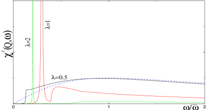
FIG. 4.: Imaginary part of the dynamical spin susceptibility in the superconducting state for $T\ll\Delta$ and $\lambda=0.5,1,2$, determined from the full solution of the Eliashberg equations. Dashed line - the normal state result shown for comparison. Observe that the resonance peak gets sharper when it moves away from $2\Delta$.

Fig.4 shows our results for $\chi({\bf Q},\omega)$ obtained from the full solution of the set of three coupled equations at $T\approx 0$ and $\lambda=0.5,1,2$. We clearly see that for $\lambda\geq 1$, the spin susceptibility has a sharp peak at $\omega=\Delta_{s}$. The peak gets sharper when it moves away from $2\Delta$. At the same time, for $\lambda=0.5$, which models weak coupling, the peak is very weak and is washed out by a small thermal damping. In this case, $\chi^{\prime\prime}$ only displays a discontinuity at $2\Delta$.

Before we proceed with the analysis of fermionic properties, we show that the spin resonance does not exist for $s-$wave superconductors. In the latter case, the spin polarization operator is given by almost the same expression as in (14), but with a different sign for $\Phi_{n}\Phi_{n+m}$ term. The sign difference comes from the fact that the two fermions in the spin polarization bubble differ in momentum by ${\bf Q}$, and the $d$-wave gap changes sign under ${\bf k}\rightarrow{\bf k}+{\bf Q}$.

One can immediately check using (14) that for a different sign of the anomalous term, $\Pi^{\prime\prime}$ does not possess a jump at $2\Delta$ (the singular contributions from $\Sigma_{n}\Sigma_{n+m}$ and $\Phi_{n}\Phi_{n+m}$ cancel each other). Then $\Pi^{\prime}(\omega)$ does not diverge at $2\Delta$, and hence there is no resonance at weak coupling. Still, however, one could naively expect the resonance at strong coupling as at small frequencies $\Pi^{\prime}(\omega)$ is quadratic in $\omega$ simply by virtue of the existence of the threshold for $\Pi^{\prime\prime}$. It turns out, however, that the resonance in the case of isotropic $s$-wave pairing is precluded by the fact that $\Pi(\omega=0)<0$ (recall that in case of $d$-wave pairing, $\Pi(\omega=0)=0$). This negative term overshadows the positive $\omega^{2}$ term in $\Pi(\omega)$ such that for all frequencies below $2\Delta$, $\Pi(\omega)<0$ [34]. That $\Pi(\omega=0)<0$ in $s-$wave superconductors can be easily explained. Indeed, a negative $\Pi(0)$ implies that the spin correlation length decreases as the system becomes superconducting. This is exactly what one should expect as $s$-wave pairing involves fermions both from opposite and from the same sublattice. The pairing of fermions from the same sublattice into a spin-singlet state obviously reduces the antiferromagnetic correlation length.

C Comparison with experiments

In Fig.5 we show the representative experimental result for $\chi^{\prime\prime}({\bf Q},\omega)$ for optimally doped ${\rm YBi}_{2}{\rm Cu}_{3}{\rm O}_{6.9}$[35]. We clearly see a resonance peak at $\omega\approx 41$ ${\rm meV}$. A very similar result has been recently obtained for ${\rm Bi}2212$[21]. In the last case, the resonance frequency is $43$ ${\rm meV}$. With underdoping, the measured resonance frequency goes down [19, 20]. In strongly underdoped ${\rm YBi}_{2}{\rm Cu}_{3}{\rm O}_{6.6}$, it is approximately $25$ ${\rm meV}$[19]. The very existence of the peak and the downturn renormalization of its position with underdoping agree with the theory. Furthermore, the measured $\chi^{\prime\prime}({\bf Q},\omega)$ displays an extra feature at $60-80$ ${\rm meV}$ [20, 35], which can be possibly explained as a $2\Delta$ effect.

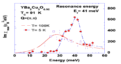
FIG. 5.: Inelastic neutron scattering intensity for momentum ${\bf Q=}\left(\pi,\pi\right)$ as function of frequency for YBa${}_{2}{\rm Cu}_{3}{\rm O}_{6.9}$. Data from Ref. [35].

The full analysis of the resonance peak requires more care as (i) the peak is only observed in two-layer materials, and only in the odd channel, (ii) the momentum dispersion of the peak is more complex than that for magnons  [36], (iii) the peak broadens with underdoping [19, 20], (iv) in underdoped materials, the peak emerges at the onset of the pseudogap, and only sharpens at $T_{c}$ [20, 35]. All these features can be explained within the spin-fermion model as well. The discussion of these effects, however, is beyond the scope of the present paper. For our present purposes, it is essential that the resonance peak has been observed experimentally, and that its frequency for optimally doped materials is around $40$ ${\rm meV}$.

We now proceed to the detailed analysis how the spin resonance at $\Delta_{s}$ affects fermionic observables. In each instance, we first briefly discuss the results for a $d-$wave gas, and then focus on the strong coupling limit.

IV “Fingerprints” of the spin resonance in fermionic variables

A The spectral function

We first consider the spectral function $A_{{\bf k}}(\omega)=(1/\pi)|G_{{\bf k}}^{\prime\prime}(\omega)|$. In the superconducting state, for quasiparticles near the Fermi surface

$$A_{{\bf k}}(\omega>0)=\frac{1}{\pi}~{}{\rm Im}\left[\frac{\Sigma(\theta,\omega)+\varepsilon_{{\bf k}}}{\Sigma^{2}(\theta,\omega)-\Phi^{2}(\theta,\omega)-\varepsilon_{{\bf k}}^{2}}\right],$$ (20)

where, we remind, $\Sigma(\theta,\omega)$ is the fermionic self-energy (which includes a bare $\omega$ term), and $\Phi(\theta,\omega)$ is a $d-$wave anomalous vertex. Both can be taken at the Fermi surface, and generally depend on the direction of ${\bf k}_{{\rm F}}$, which we labeled as $\theta$. Also, by definition, $A_{{\bf k}}(-\omega)=A_{{\bf k}}(\omega)$.

1 The $d$-wave gas

In a Fermi gas with $d$-wave pairing, $\Sigma(\theta,\omega)=\omega$, and $\Phi(\theta,\omega)=\Delta(\theta)\propto\cos\left(2\theta\right)$. The spectral function then has a $\delta-$functional peak at $\omega=(\Delta^{2}(\theta)+\varepsilon_{{\bf k}}^{2})^{1/2}$. It is obvious but essential for comparison with the strong coupling case that the peak disperses with ${\bf k}$ and far away from the Fermi surface recovers the normal state dispersion.

2 Strong coupling behavior

Here we consider the spectral function, $A_{{\bf k}}(\omega)$, for fermions located near hot spots. As we discussed, for those fermions, one can obtain a closed set of equations (Eqs.12-14) which determine $A_{{\bf k}}(\omega)$. Since spin fluctuations in a superconducting phase are propagating quasiparticles, the effect of the spin scattering on fermions near hot spots should be exactly the same as the effect of phonon scattering in an $s$-wave superconductor, i.e., in addition to a peak at $\omega=\Delta$, the spectral function $A_{{\bf k}_{{\rm hs}}}(\omega)=A(\omega)$ should possess a singularity at $\omega=\omega_{0}=\Delta+\Delta_{s}$.

The behavior of $A(\omega)$ near the singularity is very robust and can be obtained even without a precise knowledge of the frequency dependence of $\Sigma(\omega)$ and $\Phi(\omega)$. Our reasoning here parallels the one for $\Pi(\omega)$: all we need to know is that near $\omega=\Delta$, $\Sigma^{2}(\omega)-\Phi^{2}(\omega)\propto\omega-\Delta$. Substituting this form into (14) and using the spectral representation, we obtain for $\omega=\omega_{0}+\epsilon$

$$\Sigma^{\prime\prime}(\omega)\propto\int_{0}^{\epsilon}~{}\frac{dx}{(x(\epsilon-x))^{1/2}}$$ (21)

Evaluating the integral, we find that $\Sigma^{\prime\prime}$ undergoes a finite jump at $\omega=\omega_{0}$. By Kramers-Kronig relation, this jump gives rise to a logarithmic divergence of $\Sigma^{\prime}$. Exactly the same singular behavior holds for the anomalous vertex $\Phi(\omega)$, with exactly the same prefactor in front of the logarithm. The last result implies that $\Sigma(\omega)-\Phi(\omega)$ is non-singular at $\omega=\omega_{0}$. Substituting these results into (20), we find that the spectral function $A(\omega)$ emerges at $\omega>\omega_{0}$ as $1/\log^{2}(\omega-\omega_{0})$, i.e., almost discontinuously. Obviously, at a small but finite $T$, the spectral function should have a dip very near $\omega=\omega_{0}$, and a hump at a somewhat higher frequency.

FIG. 6.: (a) The quasiparticle spectral function determined by solving the coupled Eliashberg equations. The peak-dip-hump structure of $A(\omega)$ is clearly visible. (b) The real (dashed line) and imaginary (solid line) parts of the electronic self-energy. (c) The derivative of the imaginary part of the self-energy over $\omega$. The singularities at both $\Delta+\Delta_{s}$ and at $3\Delta$ are clearly seen.

In Fig.6 we present $\Sigma(\omega)$ and $A(\omega)$ from a solution of the set of three coupled Eliashberg equations at $T\approx 0$. This solution is consistent with our analytical estimate. We clearly see that the fermionic spectral function has a peak-dip-hump structure, and the peak-dip distance exactly equals $\Delta_{s}$. We also see in Fig.6 that the spectral function is nonanalytic at $\omega=3\Delta$. As we discussed, this nonanalyticity is peculiar to the spin-fermion model, and is due to the nonanalyticity of the dynamical spin susceptibility at $\omega=2\Delta$.

Another “fingerprint” of the spin-fluctuation scattering can be observed by studying the evolution of the spectral function as one moves away from the Fermi surface. The argument here goes as follows: at strong coupling, where $\Delta\geq\omega_{{\rm sf}}$, probing the fermionic spectral function at frequencies progressively larger than $\Delta$, one eventually probes the normal state fermionic self-energy at $\omega\gg\omega_{{\rm sf}}$. Due to strong spin-fermion interaction, this self-energy is large. Indeed, the solution of Eq.(14) with $\Phi=0$ and $\Pi(\omega)=i\omega$ yields at $T=0$[29]

$$\Sigma(\omega)=\omega\left(1+\frac{2\lambda}{1+(1-\frac{i|\omega|}{\omega_{{\rm sf}}})^{1/2}}\right)$$ (22)

For $\omega\gg\omega_{sf}$, $\ \Sigma(\omega)$ becomes

$$\Sigma(\omega)=\omega(1+(i{\bar{\omega}}/|\omega|)^{1/2})$$ (23)

Substituting this form into the fermionic propagator, we find that up to $\omega\sim{\bar{\omega}}$, the spectral function in the normal state does not have a quasiparticle peak at $\omega=\varepsilon_{{\bf k}}$. Instead, it only displays a broad maximum at $\omega=\varepsilon_{{\bf k}}^{2}/{\bar{\omega}}$. Alternatively speaking, at $\omega_{{\rm sf}}<\omega<{\bar{\omega}}$, the spectral function in the normal state displays a non-Fermi liquid behavior with no quasiparticle peak (see Fig. 7). This particular non-Fermi liquid behavior ($\Sigma(\omega)\propto\sqrt{\omega}$) is associated with the closeness to a quantum phase transition into an antiferromagnetic state. Indeed, at the transition point, $\omega_{{\rm sf}}=0$, and hence $\Sigma(\omega)\propto\sqrt{\omega}$ extends down to a zero frequency.

The absence of the quasiparticle peak in the normal state implies that the sharp quasiparticle peak which we found at $\omega=\Delta$ for momenta at the Fermi, cannot simply disperse with ${\bf k}$, as it does for noninteracting fermions with a $d$-wave gap. Specifically, the quasiparticle peak cannot move further in energy than $\Delta+\Delta_{s}$ as at larger frequencies, the spin scattering becomes possible, and the fermionic spectral function should display roughly the same non-Fermi-liquid behavior as in the normal state.

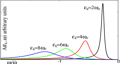
FIG. 7.: The normal state spectral function, relevant for the high frequency behavior in the superconducting state. Note the absence of a quasiparticle peak. This is the consequence of the proximity to an antiferromagnetic quantum critical point.

In Fig.8a we present successive plots for the spectral function as the momentum moves away from the Fermi surface. We see exactly the behavior we just described: the quasiparticle peak cannot move further than $\Delta+\Delta_{s}$. Instead, when ${\bf k}-{\bf k}_{{\rm F}}$ increases, it gets pinned at $\Delta+\Delta_{s}$ and gradually looses its spectral weight. At the same time, the hump disperses with ${\bf k}$ and for frequencies larger than $\Delta+\Delta_{s}$ gradually transforms into a broad maximum at $\omega=\varepsilon_{{\bf k}}^{2}/{\bar{\omega}}$. The positions of the peak and the dip versus ${\bf k}-{\bf k}_{{\rm F}}$ are presented in Fig.8b

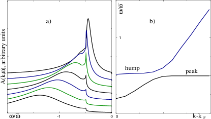
FIG. 8.: a) Frequency dependence of the spectral function in the superconducting state for different $\epsilon_{k}$. The curve at the bottom has a highest $\epsilon_{k}$. No coherent quasiparticle peak occurs for energies larger than $\Delta+\Delta_{s}$. Instead, the spectral function displays a broad maximum, similar to that in the normal state.

3 Comparison with the experiments

The quasiparticle spectral function at various momenta is measured in angle resolved photoemission (ARPES) experiments. In a sudden approximation (an electron, hit by light, leaves the crystal without further interactions with other electrons and without paying attention to selection rules for the optical transition to its final state), the photoemission intensity is given by $I_{{\bf k}}(\omega)=A_{{\bf k}}(\omega)n_{F}(\omega)$ where $n_{F}$ is the Fermi function. ARPES data of Ref.[7] for near optimally doped, $T_{c}=87{\rm K}$ in ${\rm Bi}2212$ for momenta near a hot spot are presented in Fig.9. We clearly see that the intensity displays a peak/dip/hump structure. A sharp peak is located at $\sim 40{\rm meV}$, and the dip is at $80{\rm meV}$.

FIG. 9.: ARPES spectrum  for near optimally doped Bi$2212$ for momenta close to the hot spots. Data from Ref.[6].

The experimental peak-dip distance is $42{\rm meV}$  [7]. The neutron scattering data [21] on ${\rm Bi}2212$ with nearly the same $T_{c}=91{\rm K}$ yielded $\Delta_{s}=43{\rm meV}$ which is in excellent agreement with the ARPES data. Furthermore, with underdoping, the peak-dip energy difference decreases and, up to error bars, remains equal to $\Delta_{s}$. This behavior is illustrated in Fig.10.

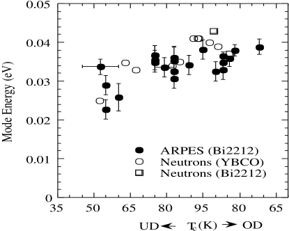
FIG. 10.: The experimental peak-dip distance at various doping concentrations vs $\Delta_{s}$ extracted from neutron measurements. Data from Ref.[30]

Finally, in Fig.11 we present experimental results for the variation of the peak and hump positions with the deviation from the Fermi surface. We clearly see that the hump disperses with ${\bf k}-{\bf k}_{{\rm F}}$ and eventually recovers the position of the broad maximum in the normal state. At the same time, the peak shows little dispersion, and does not move further in energy than $\Delta+\Delta_{s}$. Instead, the amplitude of the peak just dies off as ${\bf k}$ moves away from ${\bf k}_{{\rm F}}$. This behavior is fully consistent with the theory.

FIG. 11.: The experimental peak and hump positions with the deviation from the Fermi surface. We clearly see that the hump disperses with ${\bf k}-{\bf k}_{{\rm F}}$ and eventually recovers the position of the broad maximum in the normal state, while the peak position changes little with the deviation from ${\bf k}_{{\rm F}}$. Data from Ref.[6].

We regard the presence of the dip at $\Delta+\Delta_{s}$, and the absence of the dispersion of the quasiparticle peak are two major “fingerprints” of strong spin-fluctuation scattering in the spectral density of cuprate superconductors.

B The density of states

The quasiparticle density of states, $N(\omega)$, is the momentum integral of the spectral function:

$$N(\omega)=\int\frac{d^{2}{\bf k}}{4\pi^{2}}~{}A_{{\bf k}}(\omega).$$ (24)

Substituting $A_{{\bf k}}(\omega)$ from Eq.(20) and integrating over $\varepsilon_{{\bf k}}$, one obtains

$$N(\omega)\propto{\rm Im}~{}\int_{0}^{2\pi}d\theta~{}\frac{\Sigma(\theta,\omega)}{(\Phi^{2}(\theta,\omega)-\Sigma^{2}(\theta,\omega))^{1/2}},$$ (25)

where, we remind, $\theta$ is the angle along the Fermi surface. As before, we first consider $N(\omega)$ in a $d$-wave gas, and then discuss strong coupling effects.

1 Density of states in a $d$-wave gas

Consider for simplicity a circular Fermi surface for which $\Delta_{{\bf k}}=\Delta\cos\left(2\theta\right)$. Integrating in (25) over $\theta$ we obtain [54]

$$N(\omega) = {\rm Re}~{}\left[\frac{\omega}{2\pi}\int_{0}^{2\pi}\frac{d\theta}{\sqrt{\omega^{2}-\Delta^{2}\cos^{2}(2\theta)}}\right]$$ (26)

$$= \frac{2}{\pi}\left\{\begin{array}[]{ll}K(\Delta/\omega)&\mbox{for $\omega>\Delta$}\\ (\omega/\Delta)K(\omega/\Delta)&\mbox{for $\omega<\Delta$}\end{array}\right.,$$ (29)

where $K(x)$ is the elliptic integral of first kind. We see that $N(\omega)\sim\omega$ for $\omega\ll\Delta$ and diverges logarithmically as $(1/\pi)\ln(8\Delta/|\Delta-\omega|)$ for $\omega\approx\Delta$. At larger frequencies, $N(\omega)$ gradually decreases to a frequency independent, normal state value of the DOS, which we normalized to $1$. The plot of $N(\omega)$ in a $d-$wave BCS superconductor is presented in Fig.12

FIG. 12.: Density of states of a noninteracting Fermi gas with $d$-wave gap (solid line) and with $s$-wave gap (dashed line).

For comparison, in an $s$-wave superconductor, the DOS vanishes at $\omega<\Delta$ and diverges as $(\omega-\Delta)^{-1/2}$ at $\omega\geq\Delta$. We see that a $d$-wave superconductor is different in that (i) the DOS is finite down to the smallest frequencies, and (ii) the singularity at $\omega=\Delta$ is weaker (logarithmic). Still, however, $N(\omega)$ is singular only at a frequency which equals to the largest value of the $d-$wave gap. This illustrates a point we made earlier that the angular dependence of the $d$-wave gap reduces the strength of the singularity, but does not wash it out over a finite frequency range.

2 Density of states at strong coupling

We first show that the linear behavior of $N(\omega)$ at low frequencies and the logarithmic divergence at $\omega=\Delta$, observed in a gas, are in fact quite general and are present in an arbitrary $d-$wave superconductor. Indeed, at low frequencies ${\rm Re}\Sigma(\theta,\omega)\propto\omega$, ${\rm Re}\Phi(\theta,\omega)\propto(\theta-\theta_{{\rm node}})$ where $\theta_{{\rm node}}$ $=\frac{\pi}{4},\frac{3\pi}{4}...$ are the positions of the node of the $d$-wave gap. Substituting these forms into (25) and integrating over $\theta$ we obtain $N(\omega)\propto\omega$.  Similarly, expanding $\Sigma^{2}-\Phi^{2}$ near a hot spot, where, at least at strong coupling, the $d-$wave gap is at maximum  [32], we obtain $\Sigma^{2}(\theta,\omega)-\Phi^{2}(\theta,\omega)\propto(\omega-\Delta)+B\widetilde{\theta}^{2}$, where $\widetilde{\theta}=\theta-\theta_{{\rm hs}}$, and $B>0$.  Here, $\theta_{{\rm hs}}$ is the position of a hot spot on the Fermi surface. The integration over $\widetilde{\theta}$ then yields

$$N(\omega)\propto{\rm Re}\int\frac{d\widetilde{\theta}}{\sqrt{B\widetilde{\theta}^{2}+(\Omega-\Delta)}}\approx-\frac{\log|\Omega-\Delta|}{\sqrt{B}}.$$ (30)

This result implies that at strong coupling, the DOS in a $d-$wave superconductor still has a logarithmic singularity at $\omega=\Delta$, although the overall factor for the singular piece depends on the strength of the interaction.

We see therefore that the behavior of the density of states in a $d$-wave superconductors for $\omega\leq\Delta$ is quite robust against strong coupling phenomena. This nice universality on the other hand makes $N(\omega\leq\Delta)$ not very sensitive to a specific mechanism for the pairing.

We now demonstrate that at strong coupling, the DOS possesses extra peak-dip features, associated with the singularities in $\Sigma(\omega)$ and $\Phi(\omega)$ at $\omega=\omega_{0}=\Delta+\Delta_{s}$. The analytical consideration proceeds as follows [31]. Consider first a case when the gap is totally flat near a hot spot. At $\omega=\omega_{0}$, both $\Sigma(\omega)$ and $\Phi(\omega)$ diverge logarithmically. Substituting these forms into (25), we immediately obtain that $N(\omega)$ has a logarithmic singularity:

$$N_{{\rm sing}}(\omega)\propto\left(\log{\frac{1}{|\omega-\omega_{0}|}}\right)^{1/2}.$$ (31)

This singularity gives rise to a strong divergence of $dN(\omega)/d\omega$ at $\omega=\omega_{0}$. This behavior is schematically shown in Fig. (13)a. In part (b) of this figure we present the result for $N(\omega)$ obtained by the solution of Eliashberg-type Eqs.12-14. A small but finite temperature was used to smear out divergences. We recall that the Eliashberg set does not include the angular dependence of the gap near hot spots, and hence the result for the DOS should be compared with Fig. (13)a. We clearly see that $N(\omega)$ has a second peak at $\omega=\omega_{0}$. This peak strongly affects the frequency derivative of $N(\omega)$ which has a predicted singular behavior near $\omega_{0}$.

Note also that a relatively small magnitude of the singularity in $N(\omega)$ is a consequence of the linearization of the fermionic dispersion near the Fermi surface. For actual $\epsilon_{k}$ chosen to fit ARPES data [9], the nonlinearities in the fermionic dispersion occur at energies comparable to $\omega_{0}$. This is due to the fact that hot spots are located close to $(0,\pi)$ and related points at which the Fermi velocity vanishes. As a consequence, the momentum integration of the spectral function should have less drastic smearing effect than in our calculations, and the frequency dependence of $N(\omega)$ should more resemble that of $A(\omega)$ for momenta where the gap is at maximum.

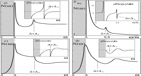
FIG. 13.: (a) The behavior of the SIN tunneling conductance (i.e., DOS) in strongly coupled $d$-wave superconductor. Main pictures - $N(\omega)$, insets - $dN(\omega)/d\omega$. (a) The schematic behavior of the DOS for a flat gap. (b) The solution of the the set of the Eliashberg-type equations for flat gap. The shaded regions are the ones in which the flat gap approximation is incorrect as the physics is dominated by nodal quasiparticles. (c) The schematic behavior of $N(\omega)$ for the quadratic variation of the gap near its maxima. (d) The expected behavior of the DOS in a real situation when singularities are softened out by finite $T$ or impurity scattering. The position of $\Delta+\Delta_{s}$ roughly corresponds to the minimum of $dN(\omega)/d\omega$.

For momentum dependent gap, the behavior of fermions near hot spots is the same as when the gap is flat, but now $\omega_{0}$ depends on $\theta$ as both $\Delta$ and $\Delta_{s}$ vary as one moves away from a hot spot. The variation of $\Delta$ is obvious, the variation of $\Delta_{s}$ is due to the fact that this frequency scales as $\Delta^{1/2}$. Since both $\Delta$ and $\Delta_{s}$ are maximal at or very near a hot spot, we can write quite generally

$$\omega_{0}\rightarrow\omega_{0}-a{\tilde{\theta}}^{2}.$$ (32)

where $a>0$. The singular pieces of the self-energy and the anomalous vertex then behave as $\log(\omega_{0}-\omega-a\widetilde{\theta}^{2})^{-1}$. Substituting these forms into (25) and using the fact that $\Sigma(\omega)-\Phi(\omega)\approx const$ at $\omega\approx\omega_{0}$, we obtain

$$N_{{\rm sing}}(\omega)\propto{\rm Re}\int d\widetilde{\theta}\left[\log(\omega_{0}-\omega-a\widetilde{\theta}^{2})^{-1}\right]^{-1/2}.$$ (33)

A straightforward analysis of the integral shows that now $N(\omega)$ has a one-sided nonanalyticity at $\omega=\omega_{0}$:

$$N_{{\rm sing}}(\omega)=-B\Theta(\omega-\omega_{0})\!\!\!~{}\left(\frac{\omega-\omega_{0}}{|\log(\omega-\omega_{0})|}\right)^{1/2},$$ (34)

where $B>0$, and $\Theta(x)=1$ for $x>0$, and $\Theta(x)=0$ for $x<0$. This nonanalyticity gives rise to a cusp in $N(\omega)$ right above $\omega_{0}$, and a one-sided square-root divergence of the frequency derivative of the DOS. This behavior is shown schematically in Fig. (13)c. Comparing this behavior with the one in Fig. (13)a for a flat gap, we observe that the angular dependence of the gap predominantly affects the form of $N(\omega)$ at $\omega\leq\omega_{0}$. At these frequencies, the angular variation of the gap completely eliminates the singularity in $N(\omega)$. At the same time, above $\omega_{0}$, the angular dependence of the gap softens the singularity, but still, the DOS sharply drops above $\omega_{0}$ such that the derivative of the DOS diverges at approaching $\omega_{0}$ from above. Alternatively speaking, in a $d-$wave superconductor, the singularity in the DOS is softened by the angular dependence of the gap, but it still holds at a particular frequency related to the maximum value of the gap. This point is essential as it enables us to read off the maximum gap value directly from the experimental data without ”deconvolution”  of momentum averages.

For real materials, in which singularities are removed by e.g., impurity scattering, $N(\omega)$ likely has a dip at $\omega\geq\omega_{0}$ and a hump at a larger frequency. This is schematically shown in Fig. (13)d. The location of $\omega_{0}$ is best described as a point where the frequency derivative of the DOS passes through a minimum.

The singularity in $dN(\omega)/d\omega$ at $\omega_{0}$, and the dip-hump structure of $N(\omega)$ at $\omega\geq\omega_{0}$ are another “fingerprints” of spin-fluctuation mechanism in the single particle response.

3 Comparison with the experiments

As we already mentioned, the fermionic DOS $N(\omega)$ is proportional to the dynamical conductance $dI/dV$ through a superconductor-insulator-normal metal (SIN) at $\omega=eV~{}$[4]. The drop in the DOS at $\omega_{0}$ can be reformulated in terms of SIN conductance as follows: if the voltage for SIN tunneling is such that $eV=\omega_{0}$, then an electron which tunnels from the normal metal, can emit a spin excitation and fall to the bottom of the band loosing its group velocity. This obviously leads to a sharp reduction of the current and produces a drop in $dI/dV$. This process is shown schematically in Fig14 [10].

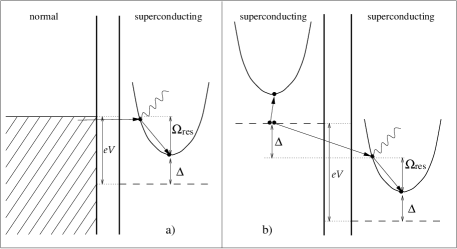
FIG. 14.: The schematic diagram for the dip features in the SIN and SIS tunneling conductances (figures a and b, respectively). For the SIN tunneling, which measures fermionic DOS, the electron which tunnels from a normal metal can emit a propagating magnons if the voltage $eV=\Delta+\Delta_{s}$. After emitting a magnon, the electron falls to the bottom of the band. This leads to a sharp reduction of the current and produces a drop in $dI/dV$. For SIS tunneling, the physics is similar, but one first has to break an electron pair, which costs energy $2\Delta$.

The SIN tunneling experiments have been performed on ${\rm YBCO}$ and ${\rm Bi}2212$ materials [14]. We reproduce these data in Fig. 15. Very similar results have been recently obtained by Pan et al [11].

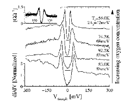
FIG. 15.: The experimental result for the differential conductance through the SIN tunneling junction. This conductance is proportional to the quasiparticle DOS. The data are for $Bi2212$ and are taken from Ref.  [14].

At low and moderate frequencies, the SIN conductance displays a behavior which is generally expected in a $d-$wave superconductor, i.e., it is linear in voltage for small voltages, and has a peak at $eV=\Delta$ where $\Delta$ is the maximum value of the $d-$wave gap [14, 11]. The value of $\Delta$ extracted from tunneling agrees well with the maximum value of the gap extracted from ARPES measurements [12, 13]. At frequencies larger than $\Delta$, the measured SIN conductance clearly displays an extra dip-hump feature which become visible at around optimal doping, and grows in amplitude with underdoping [14]. At optimal doping, the distance between the peak at $\Delta$ and the dip is around $40{\rm meV}$. This is consistent with $\Delta_{s}$ extracted from neutron measurements. The doping dependence of the peak-dip distance, and the behavior of $dN(\omega)/d\omega$ have not been studied in detail, to the best of our knowledge. This analysis is clearly called for.

C SIS tunneling

The measurements of the dynamical conductance $dI/dV$ through a superconductor - insulator - superconductor (SIS) junction is another tool to search for the fingerprints of the spin-fluctuation mechanism. The conductance through this junction is the derivative over voltage of the convolution of the two DOS [4]: $dI/dV\propto S(\omega)$ where

$$S(\omega)=\int_{0}^{\omega}d\Omega N(\omega-\Omega)~{}\partial_{\Omega}N(\Omega)$$ (35)

1 SIS tunneling in a $d$-wave gas

The DOS in a $d-$wave gas is given in Eq.(29). Substituting this form into Eq.(35) and integrating over frequency we obtain the result presented in Fig.16. At small $\omega$, $S(\omega)$ is quadratic in frequency [54]. This is an obvious consequence of the fact that the DOS is linear in $\omega$. At $\omega=2\Delta$, $S(\omega)$ undergoes a finite jump. This jump is related to the fact that near $2\Delta$, the integral over the two DOS includes the region around $\Omega=\Delta$ where both $N(\Omega)$ and $N(\omega-\Omega)$ are logarithmically singular, and $\partial_{\Omega}N(\Omega)$ diverges as $1/(\Omega-\Delta)$. The singular contribution to $S(\omega)$ from this region can be evaluated analytically and yields

$$S(\omega)=-\frac{1}{\pi^{2}}P\int_{-\infty}^{\infty}\frac{dx~{}\log|x|}{x+\omega-2\Delta}=-\frac{1}{2}\mbox{sign}(\omega-2\Delta)$$ (36)

Observe that the amplitude of the jump in the SIS conductance is a universal number which does not depend on the value of $\Delta$.

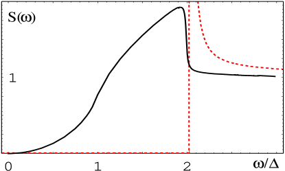
FIG. 16.: The SIS tunneling conductance, $dI/dV$, in a $d-$wave BCS superconductor. The dashed line shows $S(\omega)$ for $s$-wave case for comparison.

At larger frequencies, $S(\omega)$ continuously goes down and eventually approaches a value of $S(\omega\rightarrow\infty)=1$.

2 SIS tunneling at strong coupling

As in the previous subsection, we first demonstrate that the quadratic behavior at low frequencies and the discontinuity at $2\Delta$ survive at arbitrary coupling. Indeed, the quadratic behavior at low $\omega$ is just a consequence of the linearity of $N(\omega)$ at low frequencies. As shown above, this linearity is a general property of a $d-$wave superconductor. Similarly, the logarithmic divergence of the DOS at $\omega=\Delta$ causes the discontinuity in the SIS conductance by the same reasons as in a $d-$wave gas.

We next consider how the singularity in $\Sigma(\omega)$ at $\omega_{0}$ affects $S(\omega)$. From a physical perspective, we should expect a singularity in $S(\omega)$ at $\omega=\Delta+\omega_{0}=2\Delta+\Delta_{s}$. Indeed, to get a nonzero SIS conductance, one has to first break a Cooper pair, which costs an energy of $2\Delta$. After a pair is broken, one of the electrons becomes a quasiparticle in a superconductor and takes the energy $\Delta$, while the other tunnels. If $eV=\Delta+\omega_{0}$, the electron which tunnels through a barrier has energy $\omega_{0}$, and can emit a spin excitation and fall to the bottom of the band (see Fig. 14). This should produce a drop in $dI/dV$ by the same reasons as for SIN tunneling. This behavior is schematically shown in Fig. 17.

Consider this effect in more detail. We first notice that $\omega=\Delta+\omega_{0}$ is special for Eq.(35) because both $dN(\Omega)/d\Omega$ and $N(\omega-\Omega)$ diverge at the same energy, $\Omega=\omega_{0}$. Substituting the general forms of $N(\omega)$ near $\omega=\omega_{0}$ and $\omega=\Delta$, we obtain after simple manipulations that for a flat gap, $S(\omega)$ has a one-sided divergence at $\omega=\omega_{0}+\Delta=2\Delta+\Delta_{s}$.

$$S_{{\rm sing}}(\epsilon)\propto\frac{\Theta(-\epsilon)}{\sqrt{-\epsilon}}$$ (37)

where $\epsilon=\omega-(\omega_{0}+\Delta)$. This obviously causes the divergence of the frequency derivative of $S(\omega)$ (i.e., of $d^{2}I/dV^{2}$). This behavior is schematically shown in Fig. 17a. In Fig. 17b we present the results for $S(\omega)$ obtained by integrating theoretical $N(\omega)$ from the previous subsection (see Fig.13b). We clearly see that $S(\omega)$ and its frequency derivative are singular at $\omega=2\Delta+\Delta_{s}$, in agreement with the analytical prediction.

For quadratic variation of the gap near the maxima, the calculations similar to those for the SIN tunneling yield that $S(\omega)$ is continuous through $2\Delta+\Delta_{s}$, but its frequency derivative diverges as

$$\frac{dS(\omega)}{d\omega}\propto P\int_{0}^{\Delta}\frac{dx}{(x|\log x|)^{1/2}\left(x-\epsilon\right)}~{}\sim\frac{\Theta(-\epsilon)}{|\epsilon\log|\epsilon||^{1/2}},$$ (38)

The singularity in the derivative implies that near $\epsilon=0$

$$S(\epsilon)=S(0)-C~{}\Theta(-\epsilon)\left(\frac{-\epsilon}{|\log(-\epsilon)|}\right)^{1/2},$$ (39)

where $C>0$. This behavior is schematically presented in Fig. 17d. We again see that the angular dependence of the gap softens the strength of the singularity, but the singularity remains confined to a single frequency $\omega=2\Delta+\Delta_{s}$.

In real materials, the singularity in $S(\omega)$ is softened and transforms into a dip slightly below $2\Delta+\Delta_{s}$, and a hump at a frequency larger than $2\Delta+\Delta_{s}$. The frequency $2\Delta+\Delta_{s}$ roughly corresponds to a maximum of the frequency derivative of the SIS conductance.

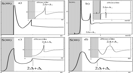
FIG. 17.: (a) The schematic behavior of the SIS tunneling conductance, $S(\omega)$, in a strongly coupled $d$-wave superconductor. Main pictures - $S(\omega)$, insets - $dS(\omega)/d\omega$. (a) The schematic behavior of $S(\omega)$ for a flat gap. (b) The solution of the the set of the Eliashberg-type equations for flat gap using the DOS from the previous subsection. The shaded regions are the ones in which the flat gap approximation is incorrect as the physics is dominated by nodal quasiparticles. (c) The schematic behavior of $S(\omega)$ for quadratic variation of the gap near its maxima. (d) The expected behavior of the SIS conductance in a real situation when singularities are softened out by finite $T$ or by impurity scattering. $2\Delta+\Delta_{s}$ roughly corresponds to the maximum of $dS(\omega)/d\omega$.

3 comparison with experiments

Recently, Zasadzinski et al.[15] obtained and carefully examined their SIS tunneling data for a set of ${\rm Bi}2212$ materials ranging from overdoped to underdoped[15]. Their data, presented in Fig.18, clearly show that besides a peak at $2\Delta$, the SIS conductance also has a dip and a hump at larger frequencies. The distance between the peak and the dip ($\approx\Delta_{s}$ in our theory) is close to $2\Delta$ in overdoped ${\rm Bi}2212$ materials, but goes down with underdoping. Near optimal doping, this distance is around $40{\rm meV}$. For underdoped, $T_{c}=74{\rm K}$ material, the peak-dip distance is reduced to about $30{\rm meV}$.

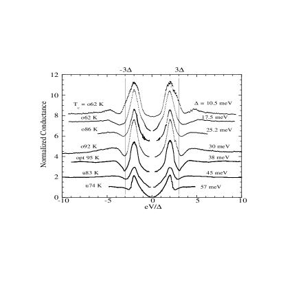
FIG. 18.: SIS tunneling data from Ref.[11] for a set of ${\rm Bi}2212$ materials ranging from overdoped to underdoped.

These results are in qualitative and quantitative agreement with ARPES and neutron scattering data, as well as with our theoretical estimates. The most important aspect is that with underdoping, the experimentally measured peak-dip distance progressively shifts down from $2\Delta$. This is the key feature of the spin-fluctuation mechanism, We regard the experimental verification of this feature in the SIS tunneling data is a strong argument in favor of a magnetic scenario for superconductivity.

D Optical conductivity and Raman response

Another observables sensitive to $\omega_{0}$ are the optical conductivity and the Raman response. Both are proportional to the fully renormalized particle-hole polarization bubble, but with different signs attributed to the bubble made of anomalous propagators. Namely, after integrating in the particle-hole bubble over $\varepsilon_{{\bf k}}$, one obtains

$$R(\omega) = {\rm Im}\int d\omega^{\prime}d\theta V^{2}(\theta)\Pi_{r}(\theta,\omega,\omega^{\prime})$$ (40)

$$\sigma(\omega) = {\rm Im}\frac{i}{\omega+i\delta}~{}\int d\omega^{\prime}d\theta\Pi_{\sigma}(\theta,\omega,\omega^{\prime})$$ (41)

where $V(\theta)$ is a Raman vertex which depends on the scattering geometry [38], and

$$\Pi_{r,\sigma}(\theta,\omega,\omega^{\prime})=~{}\frac{\Sigma_{+}\Sigma_{-}+\alpha\Phi_{+}\Phi_{-}+D_{+}D_{-}}{D_{+}D_{-}(D_{+}+D_{-})}$$ (42)

Here $\alpha=-1$ for $\Pi_{r}$, and $\alpha=1$ for $\Pi_{\sigma}$. Also, $\Sigma_{\pm}=\Sigma\left(\omega_{\pm}\right)$ and $\Phi_{\pm}=\Phi\left(\omega_{\pm}\right)$ with $\omega_{\pm}=\omega^{\prime}\pm\omega/2$ as well as $D_{\pm}=(\Phi_{\pm}^{2}-\Sigma_{\pm}^{2})^{1/2}$. Note, $\Sigma$ and $\Phi$ depend on $\omega$ and $\theta$.

1 Optical and Raman response in a $d$-wave gas

In a superconducting gas, the optical conductivity vanishes identically for any nonzero frequency due to the absence of a physical scattering between quasiparticles in a gas. The presence of a superconducting condensate, however, gives rise to a $\delta$ functional term in $\sigma$ at $\omega=0$: $\sigma(\omega)=\pi\delta(\omega)\int d\theta d\omega^{\prime}\Pi_{\sigma}(\theta,0,\omega^{\prime})$. This behavior is typical for any BCS superconductor [39], and holds for both $s-$wave and $d-$wave superconductors. The behavior of $\sigma(\omega)$ in a superconducting gas with impurities, causing inelastic scattering, is more complex and has been discussed for a $d-$wave case in, e.g., Ref.[41].

The form of the Raman intensity depends on the scattering geometry. For mostly studied $B_{1g}$ scattering, the Raman vertex has the same angular dependence as the $d$-wave gap, i.e., $V(\theta)\propto\cos\left(2\theta\right)$ [38, 40]. Straightforward computations then show that at low frequencies, $R(\omega)\propto\omega^{3}$[40]. For a constant $V(\theta)$, we would have $R(\omega)\propto\omega$.

Near $\omega=2\Delta$, the $B_{1g}$ Raman intensity is singular. For this frequency, both $D_{+}$ and $D_{-}$ vanish at $\omega^{\prime}=0$ and $\theta=0$. This causes the integral for $R(\omega)$ to be divergent. The singular contribution to $R(\omega)$ can be obtained analytically by expanding in the integrand to leading order in $\omega^{\prime}$ and in $\theta$. Using the spectral representation, we then obtain, for $\omega=2\Delta+\delta$[38]

$$R(\omega) = \int_{0}^{\epsilon}d\Omega\int d{\tilde{\theta}}~{}\frac{1}{\sqrt{\Omega+a{\tilde{\theta}}^{2}}\sqrt{\delta-\Omega+a{\tilde{\theta}}^{2}}}$$ (44)

$$\frac{1}{(\sqrt{\Omega+a{\tilde{\theta}}^{2}}+\sqrt{\delta-\Omega+a{\tilde{\theta}}^{2}})}$$

Where, as before, ${\tilde{\theta}}=\theta-\theta_{hs}$ For a flat band ($a=0$), $R(\omega)\propto Re[(\omega-2\Delta)^{-1/2}]$. For $a\neq 0$, i.e., for a quadratic variation of the gap near its maximum, the 2D integration in (44) yields $R(\omega)\propto|\log\epsilon|$. At larger frequencies $R(\omega)$ gradually decreases.

The behavior of $R(\omega)$ in a gas is shown in Fig.19. Observe that due to interplay of numerical factors, the logarithmic singularity shows up only in a near vicinity of $2\Delta$, while at somewhat larger $\omega$, the angular dependence of the gap becomes irrelevant, and $R(\omega)$ behaves as $(\omega-2\Delta)^{1/2}$, i.e., as for a flat gap.

FIG. 19.: The behavior of the Raman response in a BCS superconductor with a flat gap (dashed line), and for a quadratic variation of the gap near its maximum (solid line).

2 Raman and optical response at strong coupling

A nonzero fermionic self-energy mostly affects the optical conductivity for a simple reason that it becomes finite in the presence of the spin scattering which can relax fermionic momentum. For a momentum-independent gap, a finite conductivity emerges above a sharp threshold. This threshold stems from the fact that at least one of the two fermions in the conductivity bubble should have a finite $\Sigma^{\prime\prime}$, i.e., its energy should be larger than $\omega_{0}$. Another fermion should be able to propagate, i.e., its energy should be larger than $\Delta$. The combination of the two requirements yields the threshold for $\sigma(\omega>0)$ at $2\Delta+\Delta_{s}$, i.e., at the same frequency where the SIS tunneling conductance is singular. One can easily demonstrate that for a flat gap, the conductivity emerges above the threshold as $\epsilon^{1/2}/\log^{2}\epsilon$, where, we remind, $\epsilon=\omega-\Delta-\omega_{0}=\omega-(2\Delta+\Delta_{s})$. This singularity obviously causes a divergence of the first derivative of the conductivity at $\epsilon=+0$.

For a true $d-$wave gap, the conductivity is finite for all frequencies simply because the angular integration in Eq.(41) involves the region near the nodes, where $\Sigma^{\prime\prime}$ is nonzero down to the lowest frequencies. Still, however, we argue that the conductivity is singular at $\omega_{0}+\Delta$. Indeed, replacing, as before, $\epsilon$ by $\epsilon+\widetilde{\theta}^{2}$, substituting this into the result for the conductivity for a flat gap, and integrating over $\widetilde{\theta}$, we find that for momentum dependent gap, the conductivity itself and its first derivative are continuous at $\epsilon=0$, but the second derivative of the conductivity diverges as ${d^{2}\sigma}/{d\omega^{2}}\propto 1/(|\epsilon|\log^{2}\epsilon)$.

In Fig.20 we show the result for conductivity obtained by solving the set of coupled Eliashberg-type equations Eqs.12-14. We clearly see an expected singularity at $2\Delta+\Delta_{s}$. Note by passing that at higher frequencies, the theoretical $\Sigma(\omega)$ is inversely linear in $\omega$ [42].

FIG. 20.: Frequency dependence of the optical conductivity computed from the self energy and pairing vertex determined from the Eliashberg equations valid near hot spots. The onset of the optical response is $\omega=2\Delta+\Delta_{s}$. The contribution from the nodes (not included in calculations) yields a nonzero conductivity at all $\omega$ and softens the singularity at $\omega=2\Delta+\Delta_{s}$. The insert shows the experimental data of Puchkov et al. [16].

For the Raman intensity, the strong coupling effects are less relevant. First, one can prove along the same lines as in previous subsections that the cubic behavior at low frequencies for $B_{1g}$ scattering (and the linear behavior for angular independent vertices), and the logarithmic singularity at $2\Delta$ are general properties of a $d-$wave superconductor, which survive for all couplings. Thus, similar to the density of states and the SIS-tunneling spectrum, the Raman response below $2\Delta$ is not sensitive to strong coupling effects. Second, near $\omega_{0}+\Delta$, singular contributions which come from $\Sigma_{+}\Sigma_{-}$ and $\Phi_{+}\Phi_{-}$ terms in $\Pi_{r}$ in Eq.(41) cancel each other. As a result, we found that for a flat gap, only the second derivative of $R(\omega)$ diverges at $\Delta+\omega_{0}$. For a quadratic variation of a gap near its maximum, the singularity is even weaker and shows up only in the third derivative of $R(\omega)$. Obviously, this is a very weak effect, and its determination requires a high quality of the experiment. Notice, however, that, as we already mentioned, due to the closeness of hot spots to $(0,\pi)$ and related points, where $v_{F}$ vanishes, the smearing of the singularity due to momentum integration may be less drastic than in our theory where we used a linearized fermionic dispersion with some finite Fermi velocity.

3 Comparison with experiments

Our theoretical considerations show that optical measurements are much better suited to search for the “fingerprints” of a magnetic scenario, then Raman measurements. Evidences for strong coupling effects in the optical conductivity in superconducting cuprates have been reported in Refs. [16, 18, 45, 46]. We present the experimental data for $\sigma(\omega)$ in optimally doped ${\rm YBCO}$ in the inset of Fig.20. We see that the conductivity drops at about $100{\rm meV}$. Earlier tunneling measurements of the gap in optimally doped ${\rm YBCO}$ yielded $\Delta=29{\rm meV}$ [47]. Combining this with $\Delta_{s}=41{\rm meV}$, we find $2\Delta+\Delta_{s}\approx 100{\rm meV}$, consistent with the data. We consider this agreement as another argument in favor of a magnetic scenario.

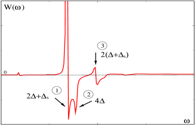
FIG. 21.: A calculated frequency dependence of $W(\omega)=\frac{d^{2}}{d^{2}\omega}(\omega{\rm Re}\sigma^{-1}(\omega))$. This quantity is a sensitive measure for fine structures in the optical response.

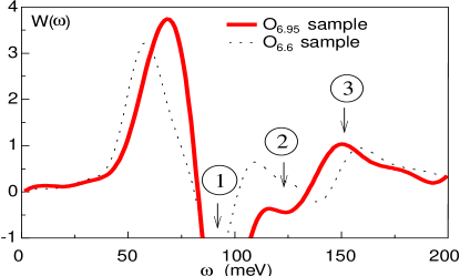
FIG. 22.: Experimental results for $W(\omega)=\frac{d^{2}}{d^{2}\omega}(\omega{\rm Re}\sigma^{-1}(\omega))$ from Ref.[18]. The position of the deep minimum agrees well with $2\Delta+\Delta_{s}$. The extrema at higher frequencies are consistent with $4\Delta$ and $2\left(\Delta+\Delta_{s}\right)$ predicted by the theory.

4 Fine structure of optical conductivity

We now argue that the measurements of optical conductivity allow one not only to verify the magnetic scenario, but also to independently determine both $\Delta_{s}$ and $\Delta$ in the same experiment. We discussed several times above that in a magnetic scenario, the fermionic self-energy is singular at two frequencies: at $\omega_{0}=\Delta+\Delta_{s}$, which is the onset frequency for spin-fluctuation scattering near hot spots, and at $\omega=3\Delta$, where fermionic damping near hot spots first emerges due to a direct four-fermion interaction. We argued that in the spin-fluctuation mechanism, both singularities are due to the same underlying interaction, and their relative intensity can be obtained within a model.

In general, the singularity at $3\Delta$ is much weaker at strong coupling, and can be detected only in the analysis of the derivatives of the fermionic self-energy. We remind that the singularity in $\Sigma(\omega)$ at $\omega_{0}$ gives rise to singularity in the conductivity at $\Delta+\omega_{0}$, while the $3\Delta$ singularity in $\Sigma(\omega)$ obviously causes a singularity in conductivity at $\omega=4\Delta$. Besides, we should also expect a singularity in $\sigma(\omega)$ at $2\omega_{0}$, as at this frequency both fermions in the bubble have a singular $\Sigma(\omega_{0})$.

For phonon superconductors, a fine structure of optical conductivity has been analyzed by studying a second derivative of conductivity via $W(\omega)=\frac{d^{2}}{d^{2}\omega}(\omega{\rm Re}\sigma^{-1}(\omega))$ which is proportional to $\alpha^{2}(\omega)F(\omega)$ where $\alpha(\omega)$ is an effective electron-phonon coupling, and $F(\omega)$ is a phonon DOS  [43].

In Fig.21 we present the theoretical result for $W(\omega)$ in our model [48]. First, we clearly see that there is a sharp maximum in $W(\omega)$ near $2\Delta+\Delta_{s}$, which is followed by a deep minimum. This form is consistent with our analytical observation that for a flat gap (which we used in our numerical analysis), the first derivative of conductivity diverges at $\omega=2\Delta+\Delta_{s}$. At a finite $T$ which is a necessary attribute of a numerical solution, the singularity is smoothened, and the divergence is transformed into a maximum. Accordingly, the second derivative of the conductivity should have a maximum and a minimum near $2\Delta+\Delta_{s}$. We found from our numerical analysis that the maximum shifts to lower frequencies with increasing $T$, but the minimum moves very little from $2\Delta+\Delta_{s}$, and is therefore a good measure of a magnetic “fingerprint”.

Second, we see from Fig.21 that besides the maximum and the minimum near $2\Delta+\Delta_{s}$, $W(\omega)$ has extra extrema at $4\Delta$ and $2\omega_{0}=2\Delta+2\Delta_{s}$. These are precisely the extra features that we expect, respectively, as a primary effect due to a singularity in $\Sigma(\omega)$ at $\omega=3\Delta$, and as a secondary effect due to a singularity in $\Sigma(\omega)$ at $\omega=\omega_{0}$.

The experimental result for $W(\omega)$ shown in Fig.22. We see that the theoretical and experimental plots of $W(\omega)$ look rather similar. Furthermore, the relative intensities of the peaks are at least qualitatively consistent with the theory. Identifying the extra extrema in the experimental $W(\omega)$ with $4\Delta$ and $2\Delta+2\Delta_{s}$, respectively, we obtain $4\Delta\sim 130{\rm meV}$, and $2\Delta+2\Delta_{s}\sim 150{\rm meV}$. This yields $\Delta\sim 32{\rm meV}$, in good agreement with earlier measurements [49], and $\Delta_{s}\sim 45{\rm meV}$, which is only slightly larger than the resonance frequency extracted from neutron measurements [19, 21]. Despite the fact that the determination of a second derivative of a measured quantity is a very subtle procedure, the very presence of the extra peaks and the fact that their positions fully agree with the theory, is an indication that the fine structures in the optical response may indeed be due to strong spin fermion scattering.

V comparison with other works

We now discuss how our work is related to other studies. As we stated in the very beginning of the paper, the fact that the interaction with a bosonic mode with frequency $\omega_{0}$ gives rise to a fermionic damping in a superconductor above $\omega_{0}+\Delta$, is known for conventional $s-$wave superconductors.[5, 44] (see also [23] and [55]). Recent angle-integrated photoemission data for lead and niobium [17] clearly demonstrated that the photoemission intensity at low $T$ possesses peak-dip features, but the dip is located well above $3\Delta$.

The reduction of the spin damping below $2\Delta$ in a $d-$wave superconductor has been discussed in [50]. It has also been argued earlier that the interaction with a nearly resonant collective mode peaked at ${\bf Q}$ explains the ARPES data. Qualitative arguments for this have been displayed by Shen and Schrieffer [51] and Norman and Ding[52]. Norman and Ding also conjectured that the peak-dip separation may be related to the frequency of a neutron peak, and presented weak-coupling calculations for a model in which fermions interact with a resonance bosonic mode. The results of this analysis agree with the ARPES data. From this perspective, the novelty of our approach is in that it presents controlled strong-coupling calculations for a low-energy spin-fermion model, which verify and extend earlier ideas.

It has been also realized earlier that in a $d-$ wave BCS superconductor, the dynamical spin response at wave vector ${\bf Q}$ contains an excitonic pole below $2\Delta$. This has been demonstrated by a number of researchers [53]. The earlier studies, however, considered a weak coupling limit, when a bare particle-hole bubble (a building block of RPA series) is made out of free fermions. However, as we discussed in Sec. III, performing weak coupling calculations consistently, one finds $\Delta_{s}$ exponentially close to $2\Delta$, and the exponentially small residue of the resonance peak. Our work extends the idea that the neutron resonance is a spin exciton to the strong coupling limit.

The results for the density of states, the SIS tunneling conductance, the Raman intensity, and the optical conductivity in a $d-$wave gas have been studied in detail by a number of researchers [54]. In our approach, we used these results as a zero-order theory, and considered strong coupling feedback effects on top of it. As far as we know, for DOS, SIS tunneling and Raman intensity, these feedback effects have not been studied before. The form of the optical conductivity and of $W(\omega)$ in cuprates has been recently studied by Carbotte and co-workers [18, 55, 56]. They also argued that the analysis of $W(\omega)$ supports a magnetic scenario for the pairing. There is, however, some discrepancy between Ref. [18] and out work: it was argued in [18] that the largest, broad maximum in $W(\omega)$ is shifted down from $2\Delta+\Delta_{s}$ due to the angular dependence of the gap, and is located at $\Delta+\Delta_{s}$. We also found that the broad maximum in $W(\omega)$ is located at a frequency smaller than $2\Delta+\Delta_{s}$. We however, attribute this reduction to finite $T$. We showed in the text that for $T\ll\Delta$, the singularity in $W(\omega)$ in a $d-$wave superconductor is still located precisely at $2\Delta+\Delta_{s}$.

Finally, several groups  [57] recently suggested phenomenologically that there is a connection between neutron resonance and specific heat anomaly in cuprates [58]. The verification of this connection within the spin-fermion model is called for.

VI Conclusions

In this paper we demonstrated that the same feedback effect which in the past allowed one to verify the phononic mechanism of a conventional, $s$-wave superconductivity, is also applicable to cuprates, and may allow one to experimentally detect the “fingerprints” of the pairing mechanism in high $T_{c}$ superconductors. We argued that for spin-mediated fermionic scattering, and for the hole-like normal state Fermi surface, the fermionic spectral function, the density of states, the SIS tunneling conductance, and the optical conductivity are affected in a certain way by the interaction with collective spin excitations which in the superconducting state are propagating, magnon-like quasiparticles with the gap $\Delta_{s}$. We have shown that the interaction with propagating spin excitations gives rise to singularities at frequencies $\Delta+\Delta_{s}$ for the spectral function near hot spots and the DOS, and at $2\Delta+\Delta_{s}$ for the SIS tunneling conductance and the optical conductivity. We demonstrated that the value of $\Delta_{s}$ extracted from these experiments agrees well with the results of neutron experiments which measure $\Delta_{s}$ directly.

We further argued that in optical measurements one can also detect subleading singularities at $4\Delta$ and $2\Delta+2\Delta_{s}$, and that these fine features have been observed at right frequencies.

We consider the experimental detection of these singularities, particularly fine structure effects, as the strong evidence in favor of the magnetic scenario for superconductivity in the cuprates.

It is our pleasure to thank A. M. Finkel’stein and D. Pines for stimulating discussions on numerous aspects of strong coupling effects in cuprates. We are also thankful to D. Basov, G. Blumberg, J.C. Campuzano, P. Coleman, L.P. Gor‘kov, P. Johnson, R. Joynt, B. Keimer, D. Khveschenko, G. Kotliar, A. Millis, M. Norman, S. Sachdev, Q. Si, O. Tchernyshyov, A.Tsvelik, and J. Zasadzinski for useful conversations. We are also thankful to D. Basov and J. Zasadzinski for sharing their unpublished results with us. The research was supported by NSF DMR-9979749 (Ar. A and A. Ch.), and by the Ames Laboratory, operated for the U.S. Department of Energy by Iowa State University under contract No. W-7405-Eng-82 (J.S).

REFERENCES

- [1] D. A. Wollmann, D. J. Van Harlingen, W. C. Lee, D. M. Ginsberg, and A. J. Leggett, Phys. Rev. Lett. 71, 2134 (1993).
- [2] C. C. Tsuei, J. R. Kirtley, C. C. Chi, Lock See Yu-Jahnes, A. Gupta, T. Shaw, J. Z. Sun, and M. B. Ketchen Phys. Rev. Lett. 73, 593 (1994).
- [3] For experimental evidences in favor of wave pairing in electron-doped cuprates, see C.C. Tsuei, J.R. Kirtley, cond-mat/0002341; R. Prozorov, R. W. Giannetta, P. Fournier, R. L. Greene, cond-mat/0002301.
- [4] G.D. Mahan, Many-Particle Physics, Plenum Press, 1990.
- [5] D. J. Scalapino, The electron-phonon interaction and strong coupling superconductors, in Superconductivity, in Superconductivity, Vol. 1, p. 449, Ed. R. D. Parks, Dekker Inc. N.Y. 1969.
- [6] see e.g., P. Monthoux, A. Balatsky and D. Pines, Phys. Rev. B 46, 14803 (1992); D.J. Scalapino, Phys. Rep. 250, 329 (1995).
- [7] M. R. Norman et al., Phys. Rev. Lett. 79, 3506 (1997).
- [8] Z-X. Shen et al, Science 280, 259 (1998).
- [9] M. R. Norman, Phys. Rev. B 61, 14751 (2000).
- [10] Strictly speaking, this argumentation is valid only when the anomalous vertex function is independent on frequency [31]. When depends on frequency and possesses the same singularity as (as in the solution of the Eliashberg set), the DOS may even diverge at approaching from below. In any situation, however, it sharply drops above .
- [11] S. H. Pan, E. W. Hudson, K. M. Lang, H. Eisaki, S. Uchida, J. C. Davis, Nature, 403, 746 (2000). More recently, these authors showed that the tunneling gap has a relatively large spatial variation, which may be the reason for the broadening of the superconducting peak observed in photoemission, (J. C. Davis, unpublished).
- [12] A.V. Fedorov et al, Phys. Rev. Lett. 82, 2179 (1999); T. Valla et al., Science, 285, 2210 (1999).
- [13] A. Kaminski et al, Phys. Rev. Lett. 84, 1788 (2000).
- [14] Ch. Renner et al., Phys. Rev. Lett. 80, 149 (1998); Y. DeWilde et al, ibid 80, 153 (1998).
- [15] J. F. Zasadzinski, L. Ozyuzer, N. Miyakawa, K.E. Gray, D.G. Hinks and C Kendzora, submitted to Science.
- [16] A. V. Puchkov et al. J. Phys. Chem. Solids 59, 1907 (1998); D. N. Basov, R. Liang, B. Dabrovski, D. A. Bonn, W. N. Hardy, and T. Timusk, Phys. Rev. Lett. 77, 4090 (1996).
- [17] A. Chainani et al, Phys. Rev. Lett. 85, 1966 (2000) and references therein.
- [18] J. P. Carbotte, E. Schachinger, D. N. Basov, Nature (London) 401, 354 (1999).
- [19] H.F. Fong et al, Phys. Rev. B 54, 6708 (1996);
- [20] P. Dai et al, Science 284, 1344 (1999).
- [21] H.F. Fong et al, Nature 398, 588 (1999).
- [22] T. Holstein, Phys. Rev. 96, 535 (1954); P.B. Allen, Phys. Rev. B 3, 305 (1971).
- [23] P. Littlewood and C.M. Varma, Phys. Rev. B 46, 405 (1992).
- [24] D. J. Scalapino, J. R. Schrieffer and J. W. Wilkins, Phys. Rev. 148, 263 (1966).
- [25] Eliashberg G.M. Sov. Phys. JETP 11, 696 (1960).
- [26] W. L. McMillan and J. M. Rowell, Tunneling and Strong Coupling Superconductivity, in Superconductivity, Vol. 1, p. 561, Ed. Parks, Marull, Dekker Inc. N.Y. 1969; W. Shaw and J.C. Swihart, Phys. Rev. Lett., 20, 1000 (1968).
- [27] D. Coffey, Phys. Rev. B 42, 6040 (1990).
- [28] A.B. Migdal, Sov. Phys. JETP, 7, 996 (1958).
- [29] A. Chubukov, Europhys. Lett. 44, 655 (1997).
- [30] Ar. Abanov and A. Chubukov, Phys. Rev. Lett., 83, 1652 (1999).
- [31] Ar. Abanov and A. Chubukov, Phys. Rev. B 61 ,R9241 (2000).
- [32] Ar. Abanov, A. Chubukov, and A. M. Finkel’stein, cond-mat/9911445.
- [33] Ar Abanov, A. V. Chubukov, and J. Schmalian, cond-mat/0005163.
- [34] Ar. Abanov, A. Chubukov, and O. Tchernyshyov, unpublished.
- [35] P. Bourges et al, cond-mat/9902067.
- [36] P. Bourges et al, Science 288, 1234 (2000).
- [37] J. C. Campuzano et al., Phys. Rev. Lett 83, 3709 (1999).
- [38] see e.g. A. Chubukov, G. Blumberg, and D. Morr, Solid State Comm. 112, 183 (1999).
- [39] J. R. Schrieffer, Theory of Superconductivity (Benjamin, Reading, Mass., 1966).
- [40] T.P. Devereaux et al., Phys. Rev. Lett. 72, 396 (1994); Phys. Rev. B 54, 12 523 (1996).
- [41] S. M. Quinlan, P. J. Hirschfeld, D. J. Scalapino, Phys. Rev. B 53, 8575 (1996).
- [42] R. Haslinger, A. Chubukov, and Ar. Abanov, cond-mat/0009051
- [43] B. Farnworth and T. Timusk, Phys. Rev. B 10, 2799 (1974); F. Marsiglio et al., Phys. Lett. A 245 , 172 (1998).
- [44] J. P. Carbotte, Rev. Mod. Phys. 62, 1027 (1990).
- [45] D. A. Bonn, P. Dosanjh, R. Liang, and W. N. Hardy, Phys. Rev. Lett. 68, 2390 (1992).
- [46] M. C. Nuss, P. M. Mankiewich, M. L. M’OMalley, and E. H. Westwick, Phys. Rev. Lett. 66, 3305 (1991).
- [47] I. Maggio-Aprile, Ch. Renner, A. Erb, E. Walker, and Ø. Fischer, Phys. Rev. Lett.75, 2754 (1995).
- [48] Ar. Abanov, A. Chubukov, and J. Schmalian, in preparation.
- [49] N. Miyakawa et al, Phys. Rev. Lett. 83, 1018 (1999).
- [50] B.W. Statt and A. Griffin, Phys. Rev. B 46, 3199 (1992); S.M. Quinlan, D.J. Scalapino and N. Bulut, ibid 49, 1470 (1994).
- [51] Z-X. Shen and J.R. Schrieffer, Phys. Rev. Lett. 78, 1771 (1997).
- [52] M.R. Norman and H. Ding, Phys. Rev. B 57 R11089 (1998); see also M. Eschrig and M.R. Norman, cond-mat/0005390.
- [53] D.Z. Liu, Y. Zha and K. Levin, Phys. Rev. Lett. 75, 4130 (1995); I. Mazin and V. Yakovenko, ibid 75, 4134 (1995); C. Stemmann, C. Pépin, and M. Lavagna, Phys. Rev. B 50, 4075 (1994); A. Millis and H. Monien, Phys. Rev. B 54, 16172 (1996); N. Bulut and D. Scalapino, Phys. Rev. B 53, 5149 (1996); J. Brinckmann and P.A. Lee, Phys. Rev. Lett. 82, 2915 (1999); S. Sachdev and M. Vojta, Physica B 280, 333 (2000); M.R. Norman, Phys. Rev. B 61, 14781 (2000); O. Tschernyshov, M.R. Norman and A. Chubukov, cond-mat/0009072; D.K. Morr and D. Pines, Phys. Rev. Lett. 81, 1086 (1998); F. Onufrieva and P. Pfeuty, cond-mat/9903097.
- [54] Ye Sun and K. Maki, Phys. Rev. B 51, 6059 (1995) and references therein.
- [55] E. Schachinger, J. P. Carbotte, and F. Marsiglio, Phys. Rev. B 56, 2738 (1997).
- [56] F. Marsiglio, T. Startseva, and J. P. Carbotte, Physics Lett. A 245, 172 (1998).
- [57] D. J. Scalapino and S.R. White, Phys. Rev. B 58, 1347 (1998); E. Demler and S.-C. Zhang, Nature, 396, 733 (1999), B. Janko, cond-mat/9912073.
- [58] J.W. Loram et al, J. Supercond., 7, 243 (1994).