Computer Science in Physics

Abstract

This talk describes how techniques developed by Computer Scientists have helped our understanding of certain problems in statistical physics which involve randomness and “frustration”. Examples will be given from two problems that have been widely studied: the “spin glass” and the “random field model”.

1 Introduction

An important part of the area of physics known as “statistical physics” is the study of phase transitions, at which the system converts from one state to another. Most interest has centered on “second order” or “continuous” transitions, in which the property which distinguishes the two phases vanishes continuously as the transition is approached. The disappearance of the magnetization of a ferromagnet, such as iron, as the temperature is increased is generally continuous. At the other type of transition, known as “first order” or “discontinuous”, there is a jump in the properties of the system as the transition is crossed, and also a latent heat. An everyday example of a first order transition is the freezing of water.

We shall focus on magnetic transitions in this talk because (i) they can be represented by simple models amenable to numerical study, and (ii) there are many experimental systems which are describable by these models. One of the major advances in the field has been the realization that behavior in the vicinity of the transition (called the “critical point”) is “universal” [1]. This means that “critical behavior” does not depend on the microscopic details of the system but only on much more basic features such its dimensionality and symmetry. Consequently one can use relatively simple models, which can be readily simulated, to make precise comparisons with experiment. That said, it should be emphasized that universality is much better justified for clean systems than for the systems with disorder which we shall be considering in this talk. One goal of applying sophisticated algorithms from computer science to these problems will be to see if universality also holds for disordered systems.

The simplest model which describes a magnetic transition, known as the Ising model, has a variable at each site on a regular lattice which can point either “up” or “down”. This represents the orientation of the magnetic moment of an atom, and is simplified to only allow two possible orientations. We shall follow standard notation in calling these variables “spins”, labeled $S_{i}$ where $i$ denotes a lattice site. It is convenient to denote the up spin state by $S_{i}=1$ and the down spin state by $S_{i}=-1$.

Neighboring sites on the lattice interact with each other. If the interaction favors parallel alignment of the spins, it is called “ferromagnetic”, while an interaction favoring anti-parallel alignment is called “anti-ferromagnetic”. The energy (confusingly called the “Hamiltonian” in the physics literature) can therefore be written as

$$E=-\sum_{\langle i,j\rangle}J_{ij}S_{i}S_{j},$$ (1)

where the sum is over all nearest neighbor pairs of the lattice (counted once) and the interactions are labeled $J_{ij}$. If all the $J_{ij}$ are positive then the state of lowest energy (ground state) has all spins parallel (either all $+1$ or all $-1$) and is called a ferromagnet. As the temperature is increased, the net alignment of the spins, the magnetization, decreases and vanishes at a critical temperature $T_{c}$, where thermal noise, which tends to randomize the spins, overcomes the interactions, which tend to make them order.

The situation with all interactions negative is simple if the sites of the lattice can be divided into two sublattices, A and B, such that all the neighbors of A are in B and vice-versa. Such lattices are said to be “bi-partite”, and are the only type that we shall consider here. A square grid is an example of a bipartite lattice. The ground state for a bipartite lattice with negative interactions has all spins $+1$ on sublattice A and all spins $-1$ on sublattice B, or vice-versa. Such a state is called an antiferromagnet. Again the ordering decreases to zero at a critical temperature.

The problems of interest to us have two more ingredients. The first is disorder. The interactions are not all equal but are chosen in some random way. The simplest model for disorder is to pick each interaction from a probability distribution, independently of all the others. The second ingredient is “frustration” or competition between the interactions. For the model in Eq. (1) this can be incorporated by allowing the sign as well as the magnitude of the interaction to be random.

That this leads to frustration can be seen in the “toy” example in Fig. 1. This shows just four sites round a square with one anti-ferromagnetic (negative) interaction and three ferromagnetic (positive) interactions. If the spins along the bottom row and top left corner are oriented in directions which minimize the energy (as shown) the spin at the top right is “frustrated” since it receives conflicting instructions from its two neighbors. It wants to be parallel to both of them which is impossible. It is easy to see that there is frustration if there is an odd number of negative interactions round the square, which is then called a “frustrated square”.

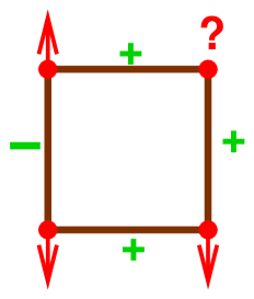
Figure 1: A simple example illustration frustration as discussed in the text.

If we extend this toy example of four sites to a large lattice, choosing the sign (and possibly the magnitude) of the interactions at random, determining the ground state is non-trivial, which is not the case if all interactions have the same sign. This type of problem, which has been extensively studied, is called a “spin glass” [2, 3]. There are many experiments on magnetic systems with these features of disorder and frustration but it would take us too far afield to discuss them here. Spin glasses are also considered as prototypes for other systems with frustration and disorder which have many features in common. Examples are neural networks, protein folding models, elastic manifolds in random media, and the “vortex glass” transition in superconductors in a magnetic field. These are discussed in the articles in Ref. [2]

Determination of the ground state in systems with disorder and frustration is an optimization problem, in which the “cost function” that has to be minimized is the energy. As we shall see, algorithms from computer science enable us to calculate the ground state of spin glasses for surprisingly large lattice sizes, at least in certain cases. An excellent introduction to optimization algorithms as applied to problems in physics is the review by Rieger [4].

Spin glasses and other problems with disorder and frustration are hard because the energy varies in a complicated manner as one moves through configuration space. There are local minima of the energy, which we will call “valleys” in the “energy landscape”, separated by “barriers” (i.e. saddle points). Different local minima can have similar energies but have very different configurations of the spins. At a finite temperature the systems should spend time in different valleys with relative proportions given by the appropriate Boltzmann factors [5]. Only one of the local minima will be the global minimum (ground state). This can be hard to find if there are many minima and/or the global minimum has a small “basin of attraction”. However, it is generally quite easy to find a minimum with energy close to the ground state energy, for example by the method of “simulated annealing” [6].

The precise value of the ground state energy will depend on the particular choice of the random interactions (remember they were picked from a distribution). In physics we usually look at “intensive” quantities (those which do not depend on size of the system, $N$, as $N\to\infty$) such as the ground state energy per spin. Many intensive quantities are “self-averaging” which means that its value does not depend on the realization of disorder for $N\to\infty$. However, there are sample-to-sample fluctuations, generally of order $1/\sqrt{N}$, for finite-sized systems, so we need to average results over many realizations of disorder. This makes the problem even more computationally challenging than if we just had to solve for one sample, but fortunately averaging over samples is clearly “trivially parallelizable”, so we can easily take advantage of the large-scale parallel machines that are widely available at present, or just run the code on a “farm” of independent workstations.

In this talk I will also discuss another widely studied problem with frustration and disorder, known as the random field model. A magnetic field will prefer a spin to align in one direction rather than the other, and so can be represented in the expression for the energy by terms linear in the spins. Eq. (1) is therefore modified to

$$E=-\sum_{\langle i,j\rangle}J_{ij}S_{i}S_{j}-\sum_{i}h_{i}S_{i},$$ (2)

where we have allowed for a different field $h_{i}$ on each site. The random field model is obtained if one chooses the $h_{i}$ at random with zero average value, and has the $J_{ij}$ unfrustrated (so we could set them all to equal unity). Again there are experimental systems which have been widely studied but which space does not allow me to discuss. For more information see Ref. [7] and the articles in Ref. [2]. In Eq. (2) frustration comes from competition between the interactions on the one hand, which prefer the spins to be parallel, and the random fields on the other, which prefer the spins to follow the local field direction.

The traditional physics approach to studying problems with frustration and disorder is the Monte Carlo simulation, i.e. a random sampling of the states according to the Boltzmann distribution [5]. However, at low temperatures the system gets trapped in one of the valleys for a long “time” and is only very rarely able to escape over a barrier in the energy landscape to another valley. The probability for escape is exponentially small in the ratio of the barrier height to the temperature. As a result, equilibrium simulations can only be done on very small systems at low temperatures. Some speed up can be obtained from recently developed Monte Carlo algorithms such as parallel tempering [8, 9] (also known as “exchange Monte Carlo”) but the range of sizes that can be studied is still quite limited.

In this talk I will discuss an alternative approach which uses sophisticated optimization algorithms from Computer Science [4] to find the exact ground state. The idea will be to “beat the small size limit” of Monte Carlo methods. The advantages of the computer science approach are:

1. It is exact. There are no statistical errors or problems of equilibration.

2. One can study large sizes.

However, there are also some disadvantages. These are:

1. Only the ground state is determined, so one is restricted to zero temperature properties.

2. Only for some models are there efficient algorithms.

In the rest of this talk I will discuss what has been learned from applying optimization algorithms to the spin glass and random field problems, and also describe some prospects for the future.

2 The Random Field Model

In this section I will discuss how optimization algorithms have enhanced our understanding of the random field model. The energy is given by Eq. (2) with the sites on a regular lattice, which we take to be a square grid in two-dimensions, a simple cubic grid in three-dimensions, and similarly in higher dimensions. The interactions $J_{ij}$ are all set to unity and the random fields are chosen from a symmetric distribution with mean and variance given by

$$[h_{i}]=0,\qquad[h_{i}^{2}]=h_{R}^{2},$$ (3)

where the rectangular brackets $[\cdots]$ denote an average over the disorder, so $h_{R}$ is the strength of the random field.

In the absence of random fields it is known that there is a non-zero magnetization $\langle S_{i}\rangle$ at low temperatures and we say that there is “long range order”. This long range order vanishes continuously at critical temperature. When the random fields are turned on one could ask whether even a small random field prevents the formation of long range order at any temperature or whether a critical field strength is needed to destroy long range order at low temperature. A famous argument due to Imry and Ma [10] states that for dimension two and lower, the random field always “wins” in the sense that long range order is destroyed by an arbitrarily weak random field, with the system “breaking up” into domains of parallel spins. The domain size diverges as $h_{R}\to 0$ so one recovers long range order for $h_{R}$ strictly zero. However, in dimension, $d$, greater than two an arbitrarily small random field does not cause the system to break up into domains on long length scales and long range order is preserved up to a critical field strength.

For $d>2$, the phase diagram is that sketched in Fig. 2. For $h_{R}=0$ the ferromagnetic phase disappears at $T=T_{c}$ due to thermal fluctuations, while at $T=0$ the ferromagnetic phase disappears at a critical value of the random field, $h_{c}$, due to the disordering effects of the random field. This will be important later.

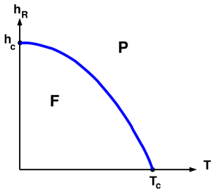
Figure 2: The phase diagram of the random field model in dimension greater than two.“P” denotes the paramagnetic phase with no long range ferromagnetic order, while “F” denotes the ferromagnetic phase.

What aspects of the random field problem are physicists interested in? It turns out that many quantities vary with a power law in the vicinity of the critical point. Denoting by $\delta$ the deviation from the phase boundary in Fig. 2, the magnetization varies, for $\delta$ small, like

$$\langle S_{i}\rangle\sim|\delta|^{\beta},$$ (4)

where $\beta$ is known as a “critical exponent”. Other quantities of interest are the specific heat, $C$, and the magnetic susceptibility, $\chi$, which vary as

$$\langle C\rangle \sim \delta^{-\alpha},$$

$$\langle\chi\rangle \sim \delta^{-\gamma}.$$ (5)

Critical exponents such as $\alpha,\beta$ and $\gamma$ are of interest because they are universal [1], only depending on broad features of the problem such as the dimensionality of the lattice and whether or not there is a random field. They are not expected to depend on the strength of the random field, as long as it is non-zero, or the distribution used for the random fields, as long as it is symmetric.

Physicists would like to the understand universal critical behavior, such as the values of the critical exponents. Since the phase boundary is crossed at zero temperature by varying $h_{R}$ one can investigate the behavior near the phase boundary using optimization (i.e. $T=0$) algorithms. Fortunately, determining the ground state energy is equivalent to a Max-Flow problem [4] which can be solved in polynomial time. This was first realized by Barahona and Anglès d’Auriac et al. [11] and subsequently used by Ogielski [12], Sourlas and collaborators [13], and others.

Here I will just discuss briefly some of the results found in Ref. [13], which investigated the random field model in $d=3$. In their optimized implementation of the Max-Flow algorithm, they studied $L^{3}$ lattices up to $L=90$, and found empirically that the CPU time varied as $L^{4}$. This is remarkably efficient, being not much more than the time ($L^{3}$) needed to scan once through the lattice. Ref. [13] provides strong evidence that the transition is actually discontinuous, corresponding to an exponent $\beta=0$. This had been suspected earlier from finite-$T$ Monte Carlo simulations [14] on sizes up to $L=16$ but the results of Ref. [13] are more convincing because they are on much larger systems. Normally a first order transition leads to a latent heat and rather weak fluctuation effects compared with a continuous transition. However, no latent heat is seen in the random field problem and, in other respects, there seem to be large fluctuation effects characteristic of a continuous transition. This dichotomy is not understood.

Several different types of random field distribution were used in Ref. [13]. While they all gave rise to $\beta=0$, other quantities, also expected to be universal, seemed to depend on the type of disorder, casting some doubt on the hypothesis that universality holds for random systems. This important question needs further work.

The $T=0$ approach cannot easily determine the specific heat exponent $\alpha$, which is unfortunate because there is a discrepancy between the experimental value [15] which is close to zero and results from Monte Carlo simulations, e.g. Ref. [14], which give $\alpha\simeq-0.5$.

3 The Spin Glass

The energy of the spin glass problem is given by Eq. (1) where the $J_{ij}$ are taken from a symmetric distribution with mean and variance given by

$$[J_{ij}]=0,\qquad[J_{ij}^{2}]=1.$$ (6)

One often takes a Gaussian distribution, though another popular choice is is the bimodal distribution, also the called $\pm J$ distribution, in which the interactions have values $+1$ and $-1$ with equal probability. The latter distribution has the special feature that there are many ground states (we say that the ground state is “degenerate”). In fact the number of ground states is exponentially large in the number of spins $N$ giving rise to a finite ground state entropy.

Two principal questions have been asked about spin glasses:

1. Is there a phase transition at finite temperature $T_{c}$?

2. What is the nature of the spin glass state below $T_{c}$?

For the first question, Monte Carlo simulations and early (unsophisticated) ground state calculations have shown;

• In $d=2$ the transition is only at $T=0$.

• In $d=3$ (and higher) the transition is at finite temperature.

The conclusion for $d=2$ is very strong and so is the situation in $d=4,5,\cdots$ etc. The case of $d=3$ has been the most difficult to resolve and earlier work was not very conclusive, but the most recent simulations [16] seem rather convincing.

Concerning the second question, we have already noted that, because of the complicated energy landscape, there are large clusters of (carefully chosen) spins which can be flipped with rather low energy cost. Is it possible to quantify this remark? Two principal scenarios have been proposed which differ, mainly, as to the energy of these large-scale excitations. These scenarios are:

• The “droplet model” of Fisher and Huse [17]. In this phenomenological picture a few very plausible assumptions are made. The lowest energy to create an excitation of linear size $L$ is assumed to vary as

  $$\Delta E\sim L^{\theta},$$ (7)

  where $\theta\ (>0)$ is an exponent. $\theta$ can not be negative if $T_{c}>0$ otherwise there would be large scale excitations which cost vanishingly small energy and the system would break up into domains at any finite temperature. We shall see below that this is what happens in $d=2$. Note that for a ferromagnet there is a positive energy cost for each interaction on the wall of the excitation and, since the wall area goes like $L^{d-1}$, one has $\theta=d-1$ in that case. However, for a spin glass it turns out that $\theta<d-1$ (in fact it is also true that $\theta<(d-1)/2$). Hence, there is a near cancellation between the effects of the bonds which were “unsatisfied” before the excitation is flipped and then become “satisfied” (which lower the excitation energy), and the the effects of the satisfied bonds which become unsatisfied (which increase the excitation energy).

• The “replica symmetry breaking” (RSB) picture of Parisi [18]. The Parisi theory is the (presumably) exact solution of an artificial model with infinite-range interactions. The assumption is then made that qualitatively similar behavior also occurs for more realistic models with short range interactions. An important ingredient of the RSB picture is that there are excitations of order the size of the system whose energy does not grow with the size of the system i.e.

  $$\Delta E\sim\mathrm{const.}$$ (8)

  This is in contrast to the prediction of the droplet theory in Eq. (7). The cancellation between the effects of the satisfied and unsatisfied bonds on the boundary of the excitation is then even more complete than in the droplet model.

To discuss what has been learned from optimization algorithms it is necessary to distinguish $d=2$ from higher dimensions. We first consider $d=2$.

We have already noted that a square is frustrated if an odd number of its bonds are negative and the converse, that the square is unfrustrated (i.e. each bond can be satisfied) if there are an even number of negative bonds, is also true. Changing the sign of the bonds in such a way that the frustration remains unchanged has no effect on the ground state energy because it can be compensated for by changing the sign of appropriate spins. Hence, for the $\pm J$ distribution, the ground state energy is determined entirely by the location of the frustrated squares. For a distribution in which the magnitude of the bonds is not constant we also need to keep track of the magnitude of the bonds (though not the sign) plus the location of the frustrated squares.

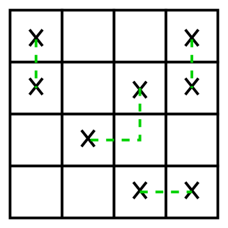
Figure 3: A two dimensional spin glass in which the frustrated squares are denoted by crosses. The ground state energy is obtained from the minimum length of the strings connecting the frustrated squares. For a distribution of interactions where the magnitude as well as the sign varies there is a weight to each string segment equal to the magnitude of the bond which it crosses.

Let us therefore indicate the frustrated squares on the lattice by drawing a cross in their center, as shown in Fig. 3. We indicate the unsatisfied bonds by drawing dashed lines at right angles across them. Clearly the lines must begin and end on frustrated squares and so form “strings” connecting the crosses. The ground state energy is increased relative to that of the unfrustrated system by the energy of the bonds crossed by the strings. For a $\pm J$ distribution the ground state energy is therefore determined by minimizing the length of the strings. For a distribution of interactions where the magnitude as well as the sign varies one has to minimize the total “weight” of the string, where the weight of a string segment is equal to the magnitude of the bond which it crosses.

This problem is equivalent to a Minimum Weight Perfect Matching Problem [4] as first realized by Barahona et al. [19] which can be solved in polynomial time, i.e. it belongs to the category “P” of optimization problems. To be more precise it is a polynomial algorithm provided the lattice is a “planar graph”, i.e. it can be drawn on a piece of paper with no lines crossing. Unfortunately this rules out periodic boundary conditions which are often imposed to eliminate surface effects which arise from the spins on the surface having a different number of neighbors from the spins in the bulk. With periodic boundary conditions the problem belongs to the class “NP”. However, an efficient “Branch and Cut” algorithm [4] enables quite large sizes to be studied [20].

In three dimensions or higher calculating the ground state of spin glass is NP for all boundary conditions. Most work has used “heuristic” algorithms, which are not guaranteed to give the exact ground states, but which, when used carefully, do seem to give the true ground state in most instances. The most effective such approach seems to be the “genetic algorithm” developed for spin glasses by Pal [21] and subsequently used by Palassini and me [22, 23] and Marinari and Parisi [24].

Let us now discuss what has been learned about spin glasses from optimization techniques, starting with $d=2$.

First we note that the restriction to $T=0$ is more serious than for the random field problem because we cannot go through the critical point. We can, however, learn about low energy excitations by computing the ground state, then perturbing the system in some way, and finally recomputing the ground state. As an example let us start with periodic boundary conditions and then change to anti-periodic boundary conditions in one direction, which simply corresponds to changing the sign of the bonds across one boundary. This induces a domain wall across the system, as shown in Fig. 4, such that all the spins on one side of the wall are flipped.

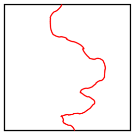
Figure 4: A domain wall crossing a two-dimensional lattice. Its energy will be of order $L^{\theta}$, where is $L$ is the size of the lattice in each dimension, and it will have a fractal dimension $d_{s}$.

The wall will have an energy, which could have either sign, and its characteristic scale varies with the size of the system in each direction, $L$, as in Eq. (7). Starting with the pioneering work of Bray and Moore [25], and followed by later studies [26, 27] for larger sizes (up to about $30^{2}$) using the Branch and Cut method, it has been found that $\theta$ is negative in $d=2$ with a value of around $-0.28$. The negative value means that the system will break up into large domains at any finite temperature, so there is no spin glass state except at $T=0$. These studies also show that the wall is a fractal with fractal dimension $d_{s}$ about 1.28, greater than 1 so it is not a smooth curve, but also less than 2 so the wall is not “space filling”.

Recently Middleton [28] has used the Matching algorithm to determine ground states of two-dimensional spin glasses with free boundaries for very large sizes, up to $512^{2}$, using a different approach to generate excitations from which $\theta$ and $d_{s}$ can be determined. His results agree well with the other work.

The case of $d=3$ is more interesting that that of $d=2$ not only because this is the physical dimension but also because there is a finite temperature spin glass state. There is general agreement that $\theta\simeq 0.20$ in $d=3$, starting with the first studies of Bray and Moore [25] which could only consider sizes up to $4^{3}$, and followed by later work [22, 29] which could go up to about $10^{3}$ using heuristic optimization algorithms. The positive value indicates that the spin glass state should be stable at low but finite temperatures. Ref. [22] also find that $d_{s}\simeq 2.68$.

Subsequently, two papers [30, 23] have argued that a different value of $\theta$, consistent with zero, is obtained from excitations in which the boundary conditions are not changed but a carefully chosen set of spins is flipped, for example by thermal noise. This suggests that the spin glass is actually quite close to the RSB picture. However, the sizes are still quite small, up to around $10^{3}$, and the assertion that there are two values (at least) for $\theta$ depending the type of excitation being considered is quite messy, so this claim needs further study.

Given the considerable interest in the spin glass in three-dimensions, it is unfortunate that there are no polynomial algorithms for finding the ground state. It is to be hoped that, in the future, algorithms will be developed which both give exact ground states and can treat larger sizes than the present heuristic algorithms.

4 Conclusions

This discussion of the role of optimization algorithms in statistical physics has been very brief. For further information the reader should consult the references. Ref. [4] is a good place to start.

The main conclusions of this talk are:

1. Algorithms from computer science have “broken the size barrier” for some problems in statistical physics, e.g.

   1. The random field model

   2. The spin glass in two-dimensions

2. The application of algorithms from computer science to physics problems works best as a collaboration between computer scientists and physicist, e.g. Ref. [26].

3. For the future I expect there will be developments in the following areas:

   1. More models will be solved.

   2. More efficient algorithms will be developed for NP problems such as the spin glass in three-dimensions. So far, with the genetic algorithm, we can study up to of order $10^{3}$ spins. Surely we do better than this.

   3. Spin glasses will be used to investigate the statistics of “hardness”. For example, given an algorithm for the exact ground state of a three-dimensional spin glass such as branch-and-cut, one can study the distribution of CPU times required to solve the problem for different realizations of disorder. It would be interesting to see how the average CPU time varies with system size and do the same for the typical (e.g. median) CPU time. If the distribution of CPU times is very broad, the average may be dominated by a few rare samples which are extremely “hard” and vary with size in a different way from the typical CPU time. This distinction has been made recently in statistical physics in the study of some quantum systems undergoing phase transitions at zero temperature [31] but, to my knowledge, does not seem to have been investigated systematically in studies of hardness of NP problems.

Acknowledgments:
I would like to thank Heiko Rieger for educating me about the algorithms mentioned in this talk and many other topics. Much of my own work in this field has been with Matteo Palassini and I would like to thank him for a stimulating collaboration. I am especially grateful to the organizer, Reinhard Wilhelm, for inviting me to speak at the 10th Anniversary Dagstuhl conference, which introduced me to large areas of computer science about which I knew nothing before. My research is supported by the NSF under grant DMR-9713977.

References

- [1] Universality became well established after the development of renormalization group theory by K. Wilson. A good reference is J. Cardy, Scaling and Renormalization in Statistical Physics, (Cambridge University Press, Cambridge, 1996).
- [2] Spin Glasses and Random Fields, A. P. Young Ed., (World Scientific, Singapore, 1998)
- [3] K. Binder and A. P. Young, Spin Glasses: Experimental Facts, Theoretical Concepts and Open Questions, Rev. Mod. Phys. 58, 801 (1986).
- [4] A good review of the application of optimization methods to problems in statistical physics is H. Rieger, Frustrated Systems: Ground State Properties via Combinatorial Optimization, in Advances in Computer Simulations, Lecture Notes in Physics, 501, J. Kertész and I. Kondor Eds., (Springer-Verlag, Heidelberg, 1998). This is also available on the cond-mat archive as cond-mat/9705010. The URL for cond-mat is http://xxx.lanl.gov/archive/cond-mat.
- [5] According to statistical mechanics, a system in thermal equilibrium has a probability proportional to of being in a state with energy , where is the temperature, and is Boltzmann’s constant (usually set to unity in model calculations). This exponential is known as a “Boltzmann factor”.
- [6] S. Kirkpatrick, C. D. Gelatt and M. P. Vecchi, Optimization by Simulated Annealing, Science 220 671 (1983).
- [7] D. P. Belanger and A. P. Young, The Random Field Ising model, J. Magn. and Magn. Mat. 100, 272 (1991).
- [8] K. Hukushima and K. Nemoto, Exchange Monte Carlo Method and Application to Spin Glass Simulations, J. Phys. Soc. Japan 65, 1604 (1996).
- [9] H. G. Katzgraber, M. Palassini and A. P. Young, Spin Glasses at Low Temperatures, cond-mat/0007113.
- [10] Y. Imry and S. K. Ma, Phys. Rev. Lett. 35, 1399 (1975).
- [11] F. Barahona, J. Phys. A. 18, L673 (1985); J.-C. Anglès d’Auriac, M. Preissman and R. Rammal, J. de Physique Lett. 46, L173 (1985).
- [12] A. T. Ogielski, Phys. Rev. Lett. 57, 1251 (1986).
- [13] N. Sourlas, Universality in Random Systems: The Case of the 3-d Random Field Ising model cond-mat/9810231; J.-C. Anglès d’Auriac and N. Sourlas, The 3-d Random Field Ising Model at Zero Temperature, Europhysics Lett. 39, 473 (1997).
- [14] H. Rieger and A. P. Young, Critical Exponents of the Three Dimensional Random Field Ising Model, J. Phys. A, 26, 5279 (1993); H. Rieger, Critical Behavior of the 3d Random Field Ising Model: Two-Exponent Scaling or First Order Phase Transition?, Phys. Rev. B 52, 6659 (1995).
- [15] D. P. Belanger, A. R. King and V. Jaccarino, Phys. Rev. B 31, 4538 (1985).
- [16] H. G. Ballesteros, A. Cruz, L.A. Fernandez, V. Martin-Mayor, J. Pech, J. J. Ruiz-Lorenzo, A. Tarancon, P. Tellez, C.L. Ullod, and C. Ungil, Critical Behavior of the Three-Dimensional Ising Spin Glass, cond-mat/0006211.
- [17] D. S. Fisher and D. A. Huse, J. Phys. A. 20 L997 (1987); D. A. Huse and D. S. Fisher, J. Phys. A. 20 L1005 (1987); D. S. Fisher and D. A. Huse, Phys. Rev. B 38 386 (1988).
- [18] G. Parisi, Phys. Rev. Lett. 43, 1754 (1979); J. Phys. A 13, 1101, 1887, L115 (1980; Phys. Rev. Lett. 50, 1946 (1983).
- [19] F. Barahona, J. Phys. A 15, 3241 (1982); F. Barahona, R. Maynard, R. Rammal and J. P. Uhry, J. Phys. A 15, 673 (1982).
- [20] The group of Prof. M. Jünger, at the University of Cologne, has generously made available to the public a server which calculates exact ground states of the Ising spin glass in two dimensions with periodic boundary conditions using a Branch and Cut algorithm. Information about this service can be obtained at http://www.informatik.uni-koeln.de/ls_juenger/projects/sgs.html.
- [21] K. F. Pal, The Ground State Energy of the Edwards-Anderson Ising Spin Glass with a Hybrid Genetic Algorithm, Physica A 223, 283 (1996); The Ground State of the Cubic Spin Glass with Short-Range Interactions of Gaussian Distribution, 233, 60 (1996).
- [22] M. Palassini and A. P. Young, Triviality of the Ground State Structure in Ising Spin Glasses, Phys. Rev. Lett. 83, 5126 (1999);
- [23] M. Palassini and A. P. Young, Nature of the Spin Glass State, Phys. Rev. Lett. 85, 3017 (2000);
- [24] E. Marinari and G. Parisi, On the Effects of a Bulk Perturbation on the Ground State of 3D Ising Spin Glasses, cond-mat/0007493; E. Marinari and G. Parisi, On the Effects of Changing the Boundary Conditions on the Ground State of Ising Spin Glasses, cond-mat/0005047;
- [25] A. J. Bray and M. A. Moore, J. Phys. C 17, L463 (1984).
- [26] H. Rieger, L. Santen, U. Blasum, M. Diehl, and M. Jünger, The Critical Exponents of the Two-Dimensional Ising Spin Glass Revisited: Exact Ground State Calculations and Monte Carlo Simulations, J. Phys. A 29, 3939 (1996).
- [27] M. Palassini and A. P. Young, Trivial Ground State Structure in the Two-Dimensional Ising Spin Glass, Phys. Rev. B. 60, R9919 (1999).
- [28] A. A. Middleton, Numerical Investigation of the Thermodynamic Limit for Ground States in Models with Quenched Disorder, Phys. Rev. Lett. 83, 1672 (1999); Energetics and geometry of excitations in random systems, cond-mat/0007375.
- [29] A. K. Hartmann, Scaling of Stiffness Energy for 3d Ising Spin Glasses, Phys. Rev. E 59, 84 (1999).
- [30] F. Krzakala and O. C. Martin, Spin and Link Overlaps in Three-Dimensional Spin Glasses, Phys. Rev. Lett, 85, 3013 (2000).
- [31] D. S. Fisher, Phys. Rev. B 51, 6411 (1995).