Grain Dynamics in a Two-dimensional Granular Flow

Abstract

We have used particle tracking methods to study the dynamics of individual balls comprising a granular flow in a small-angle two-dimensional funnel. We statistically analyze many ball trajectories to examine the mechanisms of shock propagation. In particular, we study the creation of, and interactions between, shock waves. We also investigate the role of granular temperature and draw parallels to traffic flow dynamics.

I Introduction

Density waves are known to propagate in a variety of granular flow systems. For example, flows in funnels or hoppers can have slowly propagating density waves that may move up or down depending on sand properties and geometry[1]. They also occur in long pipes[2] and closed hourglasses[3] as a result of the interaction with the interstitial fluid. In particular, they have been observed in a flow of monodisperse balls in both small-angle[4, 5] and wide-angle[6] two-dimensional funnels. In the former, one in fact observes kinematic shock waves which propagate upstream.

The kinematic shock waves in a small-angle two-dimensional funnel have a complex phenomenology of their own and have been studied extensively in a previous work [5] (hereafter referred to as HD). It was established that the flow can be divided into three different types depending on the funnel half-angle $\beta$, each having a different characteristic shock speed $U$:

• Pipe flow ($\beta<0.1^{\circ}$): the shocks can be stationary or very slow ($U<10$ cm/s) but always stop before reaching the inlet to the funnel.

• Intermittent flow ($0.1^{\circ}<\beta<0.5^{\circ}$): strong shocks propagate the full length of the funnel with $50<U<150$ cm/s.

• Dense flow ($\beta>0.5^{\circ}$): the flow is densely packed and the shocks are weak but fast ($100<U<300$ cm/s). For $\beta>2.0^{\circ}$, shocks can no longer be observed by eye.

In general, it was found that both the average local shock speed $U(x)$ and shock frequency $\nu(x)$ increased with the distance from the funnel outlet $x$. It also appeared that $U(x)\sim w(x)/D$ where $w(x)$ is the local funnel width and $D$ is the funnel outlet width. Moreover, it was established that the shocks are mainly created at specific positions as a consequence of the monodispersity. Finally, different types of interactions between shocks were also observed.

In the present work we simultaneously track all balls in the field of view of a camera to study the flow on smaller length and time scales. This enables us to observe shock creation and interaction more closely. We can then compute the granular temperature and also traffic flow curves. The paper is structured as follows. In Sec. II we describe the experimental setup and the particle tracking method. In Sec. III we study the properties of individual ball trajectories. In Sec. IV we reduce the ball flow to various one-dimensional fields. In Sec. V we discuss how shock waves are created and in Sec. VI we describe their interactions. In Sec. VII we discuss the role of granular temperature in the flow. In Sec. VIII we present the time averaged flow properties. In Sec. IX we compare the ball flow with traffic flow. Finally, we summarize our results in Sec. X.

FIG. 1.: (a) Schematic of the experiment. (b) Parameters of the funnel geometry.

II Data acquisition

A Experimental setup

The experimental setup is described in detail in HD and will only be briefly reviewed here. A top view is shown in Fig. 1(a). The granular matter consists of 50000 3.18 mm diameter brass balls. They roll in one layer between 3.45 mm high aluminum walls (A) on a coated Lexan plane (B). The aluminum walls have $200$ cm long straight sections which then open smoothly at the top forming a reservoir area (C). The straight sections can be moved to vary the outlet width $D$ and the half-angle $\beta$ of the funnel (see Fig. 1(b)). The Lexan plane is tilted an angle $\theta$ so the balls flow through the funnel into a collection container (E). Another plate (not shown) was placed on top of the aluminum walls to keep the flow in a single layer. Unless stated otherwise, the outlet width and inclination angle were kept fixed at $D=10$ mm and $\theta=4.1^{\circ}$, respectively. The funnel half-angle was varied in the range $\beta=0^{\circ}-3^{\circ}$.

Elements of the data acquisition system are also shown in Fig. 1(a). A light box (F) was placed below the lower $120$ cm of the funnel and a video camera (G) was placed above it. Its analog output signal (H) was sent to a frame grabber in a PC (not shown). The camera was mounted on a stiff bar (I) and could be moved along its length. The bar was supported by a stabilized stand (J).

B Video system

The video camera is a Pulnix TM-6701AN, $8$-bit grey tone, non-interlaced, analog CCD camera. It is capable of filming in four modes of which we used two: $640\times 200$ pixels at $130$ frames/second (fr/s) and $640\times 100$ pixels at $221$ fr/s. The camera shutter may be adjusted from no shutter to $1/32000$ s. Shutter speeds of $0.5$-$1$ ms are mostly used due to the available light intensity. The analog signal from the camera is not a standard video signal but has a pixel rate of 25.5 MHz. This signal is transmitted to a Matrix Vision PCimage SGVS frame grabber card. This PCI-bus PC-card has almost no internal memory and data is transmitted by direct memory access to the main memory of the host computer. Up to 32 MBytes may be grabbed per measurement. Thus, for $\beta<0.1^{\circ}$, up to 2000 consecutive frames may be grabbed. For the largest angles only $\sim 400$ consecutive frames can be stored. Consequently, recorded sequences typically span 2-9 s, corresponding to 1-15 shocks depending on $\beta$ and $x$.

The camera is equipped with a 16 mm C-mount lens with a field of view of $\sim 20^{\circ}$. The camera is oriented such that the $640$ pixel direction is parallel with the center line of the funnel. The view length is used to denote the length of the funnel visible in these 640 pixels. The lens was set at a height of 106 cm giving a 36.9 cm view length. The camera was placed so as to cover one of the following ranges: $x=-0.2$-36.7 cm, $x=36.8$-73.7 cm, or $x=73.8$-110.7 cm.

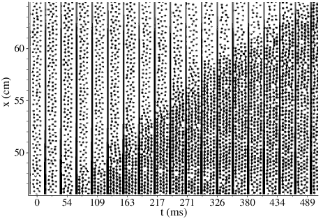
FIG. 2.: Sequence of video frames showing a propagating shock ($\beta=0.15^{\circ}$, $D=10$ mm, $\theta=4.1^{\circ}$). Only every fourth frame is shown.

The aluminum walls are painted black and extended with black plates to ensure that the only non-black part of the camera’s field of view is the funnel lighted from below. The balls therefore appear as black “dots” in a white funnel as shown in the frame sequence in Fig. 2.

C Ball tracking method

At 221 fr/s, a ball speed of 1 ball diameter per frame corresponds to a velocity of $\sim 70$ cm/s. Dense flows must be slower to be tracked. In low density flows, tracking is possible at significantly higher speeds due to the larger ball separations. (Computer based particle tracking is the only feasible method for data sets containing up to a million ball images.)

Previously, several experiments with fast, low density flows have been recorded on high speed film ($\sim 1400$ fr/s), with ball positions then obtained by eye [7]. This method is useful for following relatively small groups of particles over relatively short periods of time. Warr et al. [8] have used expensive digital high speed video equipment to follow a few (27-90) fast particles. Particle positions are subsequently determined by computer using the Hough transformation (an edge detection method [9]) for determining ball perimeters. This method requires many pixels ($\gtrsim 150$) for each ball. By comparison, we use $\sim 30$ pixels/ball.

We now sketch the algorithm used in the present experiment. (The full details are described in Appendices A and B.) Each frame is subtracted from the image of the empty funnel. Thus, the balls stand out as a white patch on a black background. A threshold is then determined based on local grey scale distributions and everything above the threshold is then defined as part of a ball. Each ball center position and height (i.e., grey scale intensity) is estimated, and a number of pixels are assigned to the ball image (typically 20-35). These data are used as input to a fitting routine. The pixel values (with coordinates $(x,y)$) are fitted to a two-dimensional peak function and the center of the fitted peak position determines the ball center ($x^{j}_{c}(t_{k})$,$y^{j}_{c}(t_{k})$) for the $j$th ball in the $k$th frame. The final result is illustrated in Fig. 3.

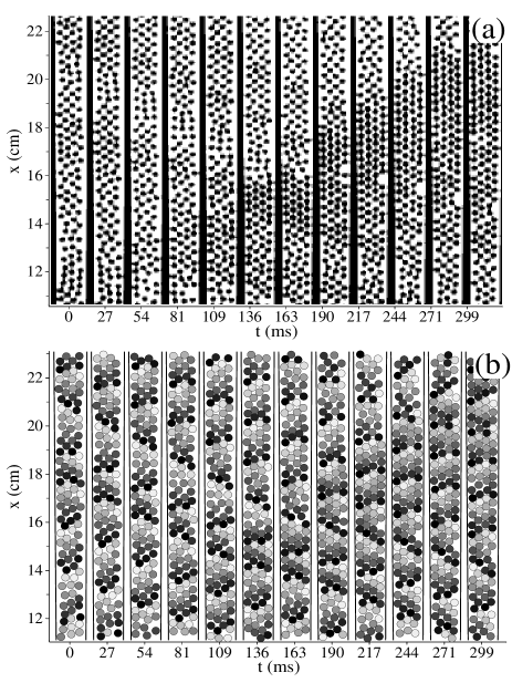
FIG. 3.: Comparison of (a) video frames and (b) corresponding artificial frames using ball tracking ($\beta=0.3^{\circ}$, $D=10$ mm, and $\theta=4.1^{\circ}$). In (b) each ball is identified by a shade of grey.

Each frame has now been converted into a table of ball positions. Based on the correlations between the first two frames and their densities, an initial guess is made of the one-dimensional coarse-grained velocity field $v(x,t_{1})$ of the first frame. The $j$th ball in the first frame is now assigned a velocity $(v^{j}_{x}(t_{1}),v^{j}_{y}(t_{1}))=(v[x^{j}_{c}(t_{1}),t_{1}],0)$. In the interest of clarity, we will henceforth drop the indices $j$ and $k$. Based on these velocities, predictions of the possible positions in the next frame are determined and compared with the actual ball positions. Positions are matched “one-to-one” making the best matches first. Balls in the old frame that cannot be matched acceptably are defined as lost. Matching is first attempted at the position predicted for constant $(v_{x}(t),v_{y}(t))$, then at the old position $(v_{x}(t),v_{y}(t))=(0,0)$, and finally at a midway point. Unmatched new balls are assigned $(v_{x}(t),v_{y}(t)=(v(x,t),0)$ at their respective positions. (In each frame $v(x,t)$ is re-computed from averages of those balls which have known velocities.) By repeated application of this method, the full trajectory of each ball can be found.

The error of $(x_{c},y_{c})$ is $\lesssim 0.15$ mm, but in a few bad cases it may be as much as $\sim 0.5$ mm. Less than $0.05\%$ of the balls are normally lost in each frame. Most balls can be followed from the time they enter the view length of the camera until they leave it. Bad matches are very rare. (They only seem to happen in groups and are easily recognized.)

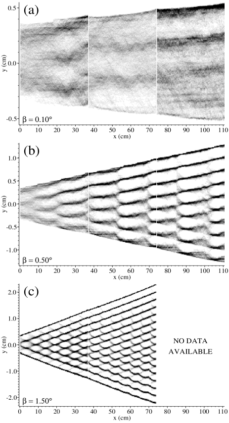
FIG. 4.: Histograms of measured ball center positions. (a) $\beta=0.1^{\circ}$. One only observes weak structures. (b) $\beta=0.5^{\circ}$. There are now $4-10$ triangular packing rows. (c) $\beta=1.5^{\circ}$. There are $4-17$ triangular packing rows. (The vertical white stripes separate independent data sets. The weak horizontal stripes in (a) and (b) with a separation of $\sim 0.6$ mm are caused by interference with camera pixel rows. See Appendix B.)

The final determination of the velocity ($v_{x}(t)$,$v_{y}(t)$) and acceleration ($a_{x}(t)$,$a_{y}(t)$) of each ball is based on a least squares fit of the positions to a parabola using a number of consecutive points. This number represents a tradeoff between precision and time resolution. For velocities, 5 points are generally used, resulting in a time resolution of $\sim 23$ ms. For accelerations, 5 or 7 points are used depending on the application. The latter corresponds to a time resolution of $\sim 32$ ms.

III Flow in Lagrangian coordinates

A Single ball trajectories

Since each measurement typically involves 0.3-1.0 million balls, it is possible to measure high resolution distributions of the ball center positions ($x_{c}(t)$,$y_{c}(t)$) (averaged over all frames). Some examples are shown in Fig. 4. For intermittent flow (Fig. 4(a)) we observe weak periodic patterns across the funnel. For dense flows (Figs. 4(b) and (c)), these patterns are much more pronounced. (No such patterns are observed for pipe flow.)

As discussed in HD, the monodispersity of the balls allows triangular close packing at packing sites $x=\chi_{i}$ given by

$$\chi_{i}=\frac{2r+\sqrt{3}r(i-1)-D}{2\tan\beta}$$ (1)

where $i$ is an integer and $r$ is the ball radius. This predicts that such packing sites should recur at intervals of $\sqrt{3}r$ and $\sqrt{3}r/2\tan\beta$ in the funnel axis and transverse directions, respectively. This is what is indeed observed as can be seen in Figs. 4(b) and (c) to within $\sim 3\%$. Immediately downstream of a packing site the lattice must rearrange itself. It appears that this occurs over a relatively short distance. For example, in Fig. 4(b) where ${\chi}_{7}=56$ cm and ${\chi}_{8}=72$ cm, the rearrangement occurs at $x=70$ cm. As one might intuitively suspect, shock waves are more readily produced where collisions are most likely. We believe this is the reason for the nearly exclusive creation of shock waves at the packing sites $\chi_{i}$ as discussed in HD.

Fig. 5(a) shows four representative examples of individual ball trajectories obtained using the method described in Sec. II C. Figs. 5(b) and (c) show $v_{x}(t)$ for the same four balls. Note that since the balls almost always move downstream, we always plot $-v_{x}(t)$ for convenience. It is apparent from these figures that an individual ball experiences long periods of constant (negative) acceleration interrupted by abrupt drops in speed to $|v_{x}|\sim 1-5$ cm/s for $\beta>0.2^{\circ}$ and $\sim 5-15$ cm/s for $\beta<0.1^{\circ}$. These drops occur when the ball encounters a shock. This qualitative behavior is even more apparent in the acceleration $a_{x}(t)$. In Fig. 6 we show the velocity $v_{x}(t)$ (a) and acceleration $a_{x}(t)$ (b) for another trajectory.

FIG. 5.: (a) The trajectories of four balls for different funnel angles. The $x_{c}(t)$-coordinate is plotted for each ball. (b) The velocity $v_{x}(t)$ of the two lower trajectories in (a) (small funnel angles). (c) The velocity $v_{x}(t)$ of the two upper trajectories in (a) (large funnel angles).

B Collisions and the coefficient of restitution

By observing collisions between two balls, we can measure (with limited resolution) the coefficient of restitution $\varepsilon$ of a ball, defined as the ratio of the relative velocities before and after a collision. This can only be done for flows with low densities and no shock waves in the field of view so that individual collisions can be identified. In two data sets at $\beta=0^{\circ}$ that adhere to these requirements, we have measured a total of 192 collisions and found that $\varepsilon=0.78\pm 0.02$. The average relative velocity before these collisions was $v_{rel}=7\pm 3$ cm/s, compared with the actual ball speed $|v_{x}|=112\pm 6$ cm/s. Assuming that the balls roll without slipping, the tangential velocity difference immediately preceding each collision should be twice the ball speed and therefore much higher than $v_{rel}$. The measured value of $\varepsilon$ using this method agrees with the value $\varepsilon\gtrsim 0.74$ found by dropping a ball on a hardened steel block.

From measurements of fast rolling collisions ($v_{x}\sim 40$-80 cm/s) with a steel barrier, we estimate $\varepsilon\sim 0.5$-0.6. The additional energy loss here may come from the rolling ball sliding on the contact surfaces at the moment of collision. This may be related to the situation where a fast ball encounters the slowly moving packed region of a shock wave.

C Shock profiles

We showed in Figs. 5(b,c) and 6(a) the velocity $v_{x}(t)$ of single ball trajectories. Their apparent sawtooth behavior is, in fact, a general feature observed in many trajectories. From this simple structure we can obtain some interesting information concerning the dissipation of the flow between shock waves.

FIG. 6.: Movement of a single ball at $\beta=0.8^{\circ}$ between $x=73$ cm and $x=37$ cm showing the (a) velocity $v_{x}(t)$ and (b) acceleration $a_{x}(t)$. The peaks in (b) indicate that the ball has encountered and is nearly stopped by a shock. The dashed line marks zero acceleration.

First, we determine the inter-shock acceleration $a_{is}$, i.e., the acceleration between shock waves. Using the acceleration $a_{x}(t)$ shown in Fig. 6(b) and employing a threshold criterion, we can identify shock waves and the time $t_{s}$ when a given ball encounters a shock wave. Linear fits yield typical values of $a_{is}=-40\pm 10$ cm/s². This value should be compared with the expected effective gravitational acceleration (for spheres rolling without slipping) $g_{r}=\frac{5}{7}g\sin{\theta}=-50$ cm/s² for $\theta=4.1^{\circ}$. It is not surprising that $|a_{is}|<|g_{r}|$ since energy is probably lost in collisions and friction processes.

FIG. 7.: Average velocity profiles of shocks in Lagrangian coordinates. Specifically, we plot the average of $-v_{x}(t-t_{s})$ of individual balls, where $t_{s}$ is a pronounced local maximum in ball acceleration. (a) $\beta=0.15^{\circ}$. Average of one shock. (b) $\beta=2.0^{\circ}$. Average of $\sim 10$ shocks. (c) single shock profile for $\beta=0.2^{\circ}$ and different inclination angles $\theta$. The dashed lines in (a) and (b) indicate the standard deviation of the measurement.

Better statistics can be obtained by averaging over many trajectories of balls encountering the same shock wave. By using a film sequence such as that in Fig. 2, we choose a time interval such that only one shock is visible in the view length. Single ball trajectories with values of $t_{s}$ within that interval are then selected (typically a few hundred). If we now average the trajectories for all these balls by setting $t_{s}=0$ for each ball, we obtain average profiles such as those shown in Figs. 7(a) and (b) for intermittent and dense flow, respectively. These preserve the sawtooth structure discussed earlier, reinforcing our picture of the behavior of single balls passing through shock waves. In particular, the inter-shock acceleration calculated for points outside the shock region for $\theta=4.1^{\circ}$ is $a_{is}=-38\pm 3$ cm/s². It was found to be independent of both velocity (i.e., the same just preceding or following a shock wave) and $\beta$ when $\beta>0.1^{\circ}$ (i.e., for intermittent and dense flows; there are exceptions in pipe flow when $|v_{x}|\gtrsim 80$ cm/s). It was also checked that $a_{is}$ was the same in different regions of the funnel, and hence independent of $x$ as it should be.

FIG. 8.: (a) The median of the distribution of $v_{min}$ versus $x$. (b) The same data replotted against the rescaled variable $w(x)/D$.

We have also checked the dependence of $a_{is}$ on $\theta$. The velocity profiles for three different values of $\theta$ are shown in Fig. 7(c). Ignoring for now differences in the velocity jumps across the shock, one sees that $a_{is}$ increases with $\theta$. For $\theta=3.0^{\circ}$, we find $a_{is}=-27\pm~{}3$ cm/s² and for $\theta=5.0^{\circ}$, $a_{is}=-45\pm~{}3$ cm/s². (These values were also independent of velocity and $\beta$.) It appears therefore that $a_{is}/g_{r}\sim 0.75$ in all three cases, implying that $a_{is}$ can be regarded as an effective gravitational acceleration.

Experiments involving only a single ball for $\theta=4.1^{\circ}$ yielded a measured value $g_{r}=-45\pm 5$ cm/s². The reason for the difference between this and the theoretical value $g_{r}=-50$ cm/s² is partially due to a local deviation of $\theta$ of $\sim 0.2^{\circ}-0.3^{\circ}$ from a small bending of the plane, and possibly also to non-ideal rolling. Consequently, we believe that the difference in $a_{is}$ and the measured value of $g_{r}$ is significant, i.e., due to the interaction between balls in intermittent and dense flows.

Just before and after a shock, a ball reaches its maximum and minimum velocity $v_{max}$ and $v_{min}$, respectively (see, for example, Fig. 6). In particular, knowledge of $v_{min}$ is necessary to understand the creation of shock waves discussed in Sec. VI. In the same manner as discussed earlier, we find that the average value of $v_{min}$ for all balls passing through a given shock wave is $|v_{min}|\sim 10-20$ cm/s, $4-10$ cm/s, and $1-5$ cm/s, in pipe, intermittent, and dense flow, respectively (see for example Figs. 5, 6, and 7).

We also checked the dependence of $v_{min}$ on $\beta$ and $x$. (Due to the presence of shock waves that are created within the view length and a low number of shock waves, $v_{min}(x)$ is obtained as the median of the distribution of $v_{min}$, not the mean.) This is shown in Fig. 8(a) for $0.4^{\circ}<\beta<3.0^{\circ}$ and $D=7$, 10, and 14 mm. (There were too few shock waves for smaller $\beta$ to obtain meaningful statistics.) In HD it was found that the local shock speed $U(x)$ depended linearly on the local funnel width $w(x)$. If we plot $v_{min}$ against $w(x)/D$, we obtain the plot shown in Fig. 8(b). The apparent collapse of the data indicates that there may indeed be some simple scaling properties inherent in the system. It will be shown in a future work how the behavior of $a_{is}$ and $v_{min}$ can be used to model shock wave statistics[10].

IV Flow in Eulerian coordinates

A Granular fields

From the full set of ball trajectories in the flow, we can construct continuous one-dimensional Eulerian fields, such as the density $\rho(x,t)$ and velocity $v(x,t)$. (The justification for considering a one-dimensional flow is given in Appendix C.) Of course, to obtain meaningful results, it is necessary to coarse-grain. In order to obtain a spatial resolution better than one ball diameter, this was done by drawing a primitive unit cell (for close-packed circles) around the ball center positions $(x_{c}(t),y_{c}(t))$, with two sides parallel to $x$ (i.e., the center line of the funnel). The funnel was then binned into strips of width $\sim 0.1$ mm and the occupied area was calculated for each strip. These strips can then be summed to achieve any desired resolution, although typically we used a resolution of $\sim 1$ mm. We then divided by the area of the strip to obtain the relative density $\tilde{\rho}(x,t)$. Thus, for close packed balls, $\tilde{\rho}(x,t)=1$. (The relative density here differs from that in HD which was measured using relative light intensities.) The velocity field $v(x,t)$ is then computed as the weighted average

$$v(x,t)=\sum_{j}\tilde{\rho}^{j}v_{x}^{j}(t)/\sum\tilde{\rho}^{j}$$ (2)

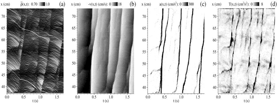
FIG. 9.: The different fields for $\beta=0.8^{\circ}$. (a) relative density $\tilde{\rho}(x,t)$, (b) velocity $v(x,t)$, (c) positive acceleration $a(x,t)$, (d) granular temperature $T(x,t)$.

where the sum is over all balls whose unit cells contribute to a strip and $\tilde{\rho}^{j}$ is the corresponding relative density. The acceleration field $a(x,t)$ is obtained in a similar manner.

The granular temperature per ball is defined as $T(x,t)=\langle(v_{y}-\bar{v}_{y})^{2}\rangle+\langle(v_{x}-\bar{v}_{x})^{2}\rangle$ where $\bar{v}_{x}=v(x,t)$ and $\bar{v}_{y}=0$, and where the brackets indicate an average as in Eq. 2. It can be written as the two components $T(x,t)={T_{x}}(x,t)+{T_{y}}(x,t)$, where ${T_{x}}(x,t)=\langle[v_{x}-v(x,t)]^{2}\rangle$ and ${T_{y}}(x,t)=\langle v_{y}^{2}\rangle$, in order to see if the granular temperature is isotropic.

B Discussion of the fields

An example of the relative density is shown in Fig. 9(a) for dense flow ($\beta=0.8^{\circ}$). It reveals five faint shocks. However, in dense flows, density fluctuations on the scale of a ball diameter tend to be comparable with or even dominate the fluctuations associated with the passing of shock waves. (For example, the whiter tracks moving downstream are defects, which are often vacancies. In dense flows they can survive the passing of shock waves since shocks do not seriously rearrange the local packing.)

The corresponding velocity and acceleration fields are shown in Figs. 9(b) and (c), respectively. In the velocity field, the same shock waves are much more clearly visible since the greatest contrast occurs when fast balls enter a shock wave and lose most of their speed. (Note that again, since $v(x,t)$ is always negative, we plot $-v(x,t)$ here and in all subsequent plots.)

By adjusting the resolution in the positive acceleration field $a(x,t)$ shown in Fig. 9(c), we can improve the contrast in $v(x,t)$ in order to reveal weaker details of the flow. For example, one can now see the creation of (temporarily) stationary shocks at locations corresponding approximately to the packing sites $\chi_{8}=45$ cm and $\chi_{9}=55$ cm (see Eq. 1).

The granular temperature $T(x,t)$ shown in Fig. 9(d) clearly peaks in the shock regions as it did for $a(x,t)$, although it is not as evenly distributed along the shocks. The temperature appears to cool down over relatively short time and length scales. There is a background level of $\sim 2$ cm${}^{2}/$s² with a weak packing site periodicity of $\sim 10$ cm. The granular temperature will be discussed more thoroughly in Sec. VII.

C Flow dynamics for fixed $x$

The grey scale plots of the granular fields in Fig. 9 do not convey the magnitudes of the fields very well. Therefore we show $v(x,t)$ and $\tilde{\rho}(x,t)$ for four fixed $x$ in Fig. 10 and study how these quantities are affected by propagating shock waves.

In Fig. 10(a), the velocity $v(x,t)$ is shown at $x=44$ cm (midway between ${\chi}_{4}=24$ cm and ${\chi}_{5}=64$ cm), and at $x=\chi_{5}=64$ cm for an intermittent flow ($\beta=0.2^{\circ}$). (These positions were chosen for reasons which will become clear later.) One can clearly see propagating shock waves and smoothly increasing flow speeds between the shocks in the range 3-45 cm/s. From the displacements of the shock fronts, we estimate that $U\sim 120$ cm/s. At $x=64$ cm, one can see two shocks labelled A1 and A2. From fields such as those in Fig. 9, we know that these are newly created shocks. At $x=44$ cm, disturbances are observed at A3 and A4 as the velocity increases between shocks. These are caused by balls that have passed the newly created shocks at A1 and A2. The corresponding relative densities are shown in Figs. 10(b,c). They reveal that the shock fronts are relatively sharp, but otherwise details of the flow are generally not as clear as in $v(x,t)$.

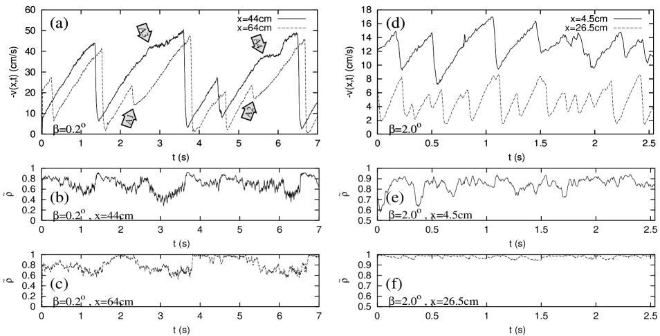
FIG. 10.: Time series of $-v(x,t)$ and $\tilde{\rho}(x,t)$ at fixed $x$ showing propagating shocks for two different $\beta$. (a) velocity for $\beta=0.2^{\circ}$ at $x=44$ cm (between $\chi_{4}$ and $\chi_{5}$) and $x=\chi_{5}=64$ cm. A1 and A2 indicate newly created shocks, and A3 and A4 show, respectively, the effect of these shocks 20 cm downstream. (b) density corresponding to (a) at $x=44$ cm. (c) density corresponding to (a) at $x=64$ cm. (d) velocity for $\beta=2.0^{\circ}$ at $x=4.5$ cm (between packing sites) and $x=26.5$ cm (at a packing site). (e) density corresponding to (d) at $x=4.5$ cm. (f) density corresponding to (d) at $x=26.5$ cm.

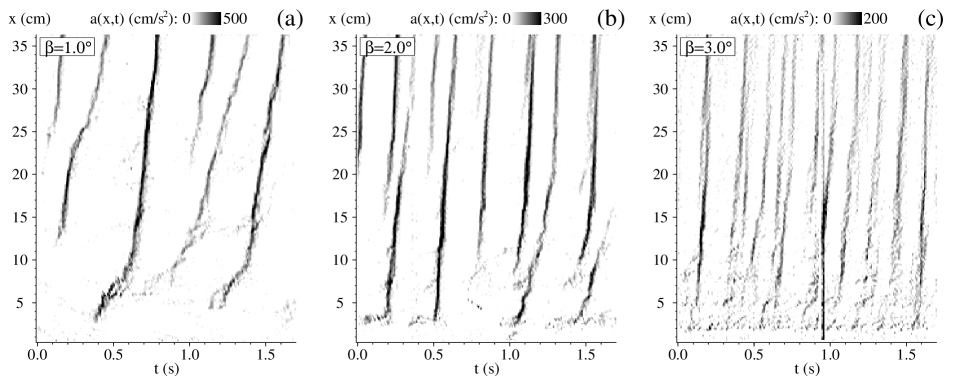
FIG. 11.: Acceleration field $a(x,t)$ showing weak shock waves for large values of $\beta$: (a) $\beta=1.0^{\circ}$, (b) $\beta=2.0^{\circ}$, (c) $\beta=3.0^{\circ}$. The grey scale for the magnitude is shown at the top of each plot.

In Fig. 10(d), we show $v(x,t)$ at $x=4.5$ cm (between ${\chi}_{4}=2.4$ cm and ${\chi}_{5}=6.5$ cm), and $x=\chi_{10}=26.5$ cm for a dense flow ($\beta=2.0^{\circ}$). Many shocks with speeds $U\sim 350$ cm/s are now visible. At $x=4.5$ cm they are all newly created. These shocks can still be observed at $x=26.5$ cm along with many other shocks created upstream of them. The corresponding relative densities are shown in Figs. 10(e) and (f), respectively. These are of limited value when $\beta>1.5^{\circ}$ Near the outlet (e) there are still fluctuations related to shock waves, but upstream (f) the density is constant and nearly unity despite the presence of many shock waves.

D Shock behavior for $\beta>1.0^{\circ}$

As $\beta$ is increased, the shock waves are faster, weaker, and more frequent as discussed in HD. For $\beta>1.5^{\circ}$, one can no longer study shock waves from directly measured density fluctuations as in HD and in this situation the ball tracking method is particularly useful.

In Figs. 11(a-c) we show $a(x,t)$ near the outlet for three relatively large values of $\beta$. One can see that as $\beta$ increases, the frequency and speed of the shocks increase while their strength decreases. In particular, in Fig. 11(c) it also appears that the shock waves die off noticeably with increasing $x$.

FIG. 12.: The spatial dependence of (a) the velocity $-v(x,t)$ and (b) the corresponding relative densities $\tilde{\rho}(x,t)$ for fixed $t$. In these data, one is observing a decaying propagating shock.

Once again it it useful to look at the magnitudes of $v(x,t)$ and $\tilde{\rho}(x,t)$, but now for fixed $t$. In Fig. 12 we show $v(x,t)$ and $\tilde{\rho}(x,t)$ for four equally spaced consecutive times. In Fig. 12(a) one can see a shock propagating upstream with a speed $U\sim 250$ cm/s. As already noted, it dies off as it moves upstream, but now one can clearly see that the shock region also gets broader. Fig. 12(b) indicates why the density $\tilde{\rho}(x,t)$ cannot be used to detect shock waves for large $\beta$. Except for the lowest 10 cm of the funnel, the density fluctuations are entirely dominated by the packing sites (which in this case have a periodicity of 3.2 cm).

FIG. 13.: (a) Estimated shock speed $U(x)$ for $1.0^{\circ}\leq\beta\leq 3.0^{\circ}$ and $D=7$, 10, and 14 mm. (b) The same data replotted against the rescaled variable $w(x)/D$.

As already discussed in Sec. III C, it was observed in HD that for $0.1^{\circ}<\beta<1.0^{\circ}$ the local average shock speed seemed to depend linearly on the local funnel width. We can now test this hypothesis for larger $\beta$. Unfortunately, with our current data constraints, we have only 10-20 shocks so the statistics are not as good as could be desired. Fig. 13 shows $U(x)$ based on a simple ridge detection method applied to $a(x,t)$. Fig. 13(a) shows $U(x)$ for different values of $\beta$ and $D$ while (b) shows the same data versus $w(x)/D$. The data collapse in Fig. 13(b) is not complete, although it is consistent with the same analysis in HD.

V Shock creation

Having established some understanding of how shock waves propagate, we would now like to examine under what circumstances they are created. Since for $\beta>0.1^{\circ}$ shock waves (once created) propagate all the way to the reservoir, the mechanisms of shock creation will strongly effect the flow properties. In HD it was found that for intermittent flows new shock waves were almost exclusively created at the packing sites $\chi_{i}$. Fig. 4 illustrates how a moderately dense flow is forced to reorganize at the packing sites, thus possibly increasing the likelihood of congestion there.

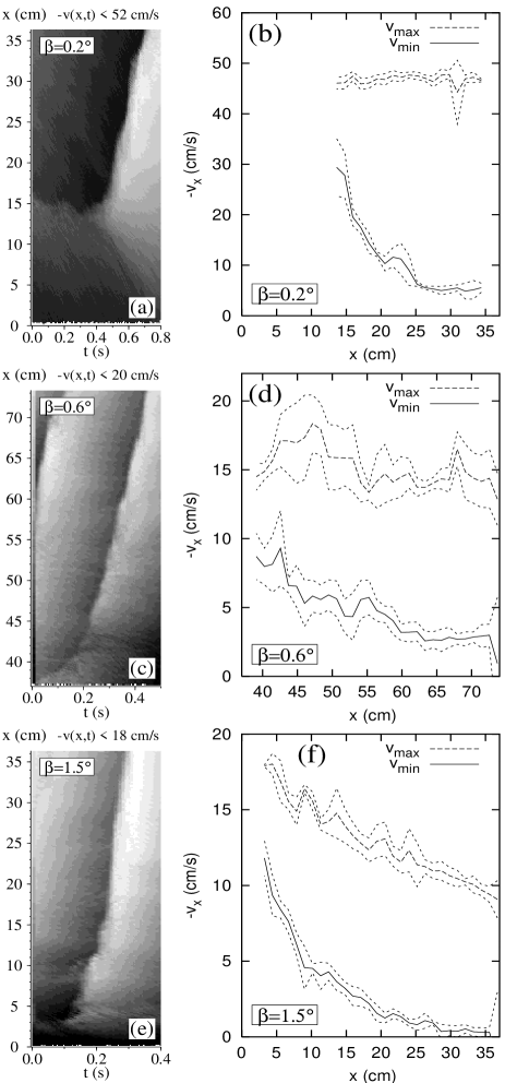
FIG. 14.: Examples of starting shocks and their respective $v_{min}(x)$ and $v_{max}(x)$ for different funnel angles: (a,b) $\beta=0.2^{\circ}$, (c,d) $\beta=0.6^{\circ}$, (e,f) $\beta=1.5^{\circ}$.

In Sec. III C it was discussed how $v_{min}$ varies in the different flow types. Basically $v_{min}$ is a measure of how effectively the shock has absorbed momentum and energy from the flow upstream of the shock. Generally, we have found that $v_{min}$ for newly created shocks is often significantly higher than the typical values of $v_{min}(x)$ shown in Fig. 10(a) where the shocks at A1 and A2 are known to be newly created. This means that the new shocks do not dissipate energy as efficiently as the older shocks around them. Three examples of newly created shocks are shown in Figs. 14(a,c,e), and the averages of $v_{min}$ and $v_{max}$ of the balls encountering these shocks are shown in (b,d,f), respectively. One can observe how $v_{min}$ starts relatively high, but then over a distance of 5-15 cm, it drops to the typical values found in Sec. III C.

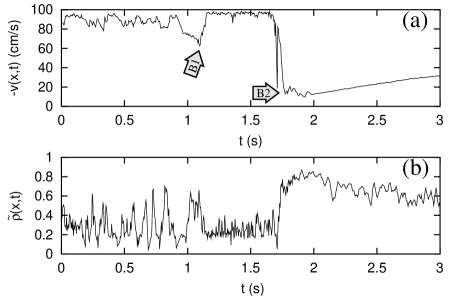
FIG. 15.: Time series of (a) $-v(x,t)$ and (b) $\tilde{\rho}(x,t)$ at $x=30$ cm showing the creation of a shock in pipe flow ($\beta=0.075^{\circ}$). A slow, dense group of balls passes downstream (B1) and forms a shock at $x=26$ cm (not shown) which starts propagating upstream (B2).

For each flow type we can make more specific observations about how shocks are typically created. In pipe flow new shocks typically start as a group of balls moving downstream which have a somewhat smaller velocity and higher density than those around them. This early stage of a shock at some point becomes stronger, stops, and then starts moving upstream as a stable shock (shocks moving downstream are generally not very stable). An example of this process is shown in Fig. 15 where a disturbance passes the observation point at B1, turns around downstream, and then starts propagating upstream, passing the observation point again at B2. Mass conservation across the shock discontinuity requires that

$$U=(\rho_{u}v_{u}-\rho_{d}v_{d})/(\rho_{u}-\rho_{d})$$ (3)

where the subscripts $u$ and $d$ signify upstream and downstream of the shock, respectively. In this example, $\rho_{u}\sim 0.3w$, $\rho_{d}\sim 0.6w\rightarrow 0.8w$, and $v_{u}\sim-95$ cm/s. Note that as $v_{d}$ increases from $-70$ cm/s to $-20$ cm/s, and $\rho_{d}$ increases slightly, $U$ changes sign.

In intermittent flow the shock may start in the manner described above for pipe flow, but more commonly it is created at a packing site without the early downstream phase discussed above. An example of such a shock is shown in Fig. 14(a).

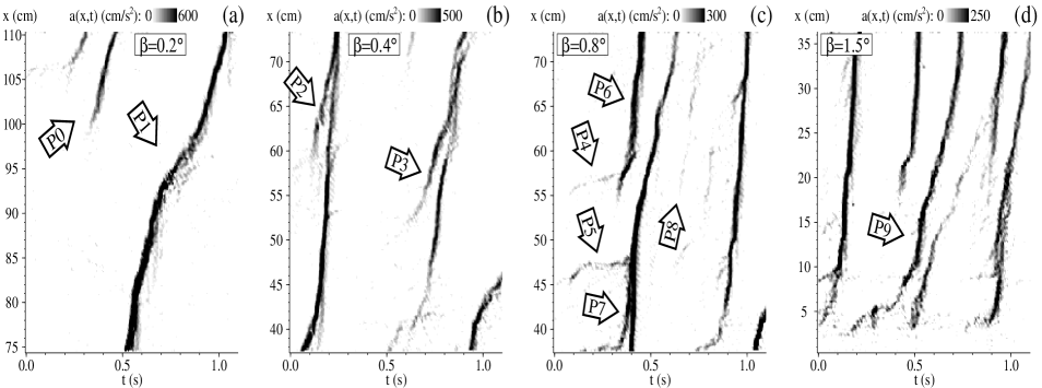
FIG. 16.: Positive acceleration field $a(x,t)$ showing examples of shock interactions. (a) Shock start repulsion (P0 and P1) ($\beta=0.2^{\circ}$). (b) Two temporary pre-shocks (P2 and P3) ($\beta=0.4^{\circ}$). (c) Stationary shocks joining at packing sites (P4 and P5), and a near shock repulsion (P6), pre-shock (P7), and micro-shock (P8) ($\beta=0.8^{\circ}$). (d) Near shock repulsion (P9) ($\beta=1.5^{\circ}$).

In Fig. 14(b) we see how the growing difference between $v_{min}$ and $v_{max}$ shows how shocks improve their ability to absorb momentum and energy during the first 10 cm of propagation. Other examples of shock creation in intermittent flows have already been shown in Figs. 3(a) and 10(a).

In dense flow shocks are often created by the joining of a few relatively stationary weak “pre-shocks” (which will be discussed in the next section) or a region with seemingly “unstructured” disturbances in the flow at a packing site (see, e.g., Figs. 9 and 11). The nature of these shock creation processes is not known. Fig. 14(c) shows the creation of a shock wave 38 cm upstream of the outlet. The $|v_{min}|$ shown in Fig. 14(d) initially has a value somewhat higher than what is typical for that funnel position (see Fig. 8(a)). In Fig. 14(e) the creation of a shock near the outlet is shown for large $\beta$. Fig. 14(f) shows how its $|v_{min}|$ also quickly drops after the creation. Near the outlet (and one packing site up) all shocks have just been created. Therefore, the $v_{min}$ curve in Fig. 14(f) partially corresponds to the first part of the curves in Fig. 8. This also explains why the values of $v_{min}$ in Fig. 10(d) at $x=4.5$ cm are relatively high.

VI Shock interactions

Shock wave interactions have been discussed in HD. Since these were studied using directly measured density fluctuations, they were hard to resolve and the nature of the interactions was somewhat speculative. The superior spatial and temporal resolution of the ball tracking method now gives us a clearer picture of the interactions and even reveals new interactions not observed earlier.

An example of a weak shock start repulsion is shown in Fig. 16(a). First, a new shock is created at point (P0). When the balls leaving this shock reach the next shock, they cause it to temporarily slow down (P1), in effect repelling it. (A similar patch of slower balls was observed in Fig. 10(a) at A3 and A4 following the creation of new shocks at A1 and A2.)

In Fig. 16(b) examples of pre-shocks (P2 and P3) separated from the main shock by less than $0.1$ s are shown. At P3 the pre-shock seems to gain amplitude and swallows the original main shock. Fig. 16(c) shows weak stationary shocks (P4 and P5) waiting to be swallowed by arriving shocks at or just upstream of packing sites. Examples are shown of a near shock repulsion at P6 and of a weak pre-shock at P7. Some micro-shocks also seem to propagate upwards with speeds similar to the surrounding shocks at P8. It is not clear what these represent, but since the balls are densely packed at $\beta=0.8^{\circ}$, they may be “chain collisions” propagating in single rows of balls. The data set in Fig. 16(c) partially overlap the data presented in Fig. 9. In Fig. 16(d) a near shock repulsion is seen at P9 and several weak waiting shocks are observed. These waiting shocks seem related to the shock creation process in dense flows discussed in Sec. V. There is no indication that shock interactions disappear at larger $\beta$ (compare with Fig. 11).

VII Shock temperature

When a ball encounters a shock, it quickly loses most of its velocity (and therefore most of its momentum and energy) in collisions with other balls and the funnel walls. In the dense region of the shock where the mean distance between balls is small, this results in relatively high collision rates when they encounter a fast incoming ball. The high density also forces balls to come into contact with the funnel walls so that the total momentum/energy of a dense group of balls is also reduced by friction. This phenomenon is reminiscent of the clustering[11] and inelastic collapse[12] observed in simulations of granular materials.

This process can also be described as follows. Upstream of the shock there is a steady flow of relatively high energy balls. When a group of balls encounters the shock, collisions “randomize” their translational energy, increasing the granular temperature. However, it is then reduced by each collision and by the friction processes mentioned above. Some distance downstream of the shock the relative motion of neighboring balls appears to be negligible. Thus, since we cannot measure collision rates in a shock, the rate at which the granular temperature decays in a group of balls following the passage of a shock front seems the best way of studying the energy loss processes in the shock. Consequently, we define $\tau_{T}$ as the characteristic decay time of $T(x,t)$ following the passage of a shock front in Lagrangian coordinates.

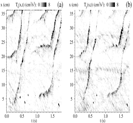
FIG. 17.: Comparison of (a) $T_{x}(x,t)$ and (b) $T_{y}(x,t)$ showing creation and propagation of shocks for $\beta=0.6^{\circ}$.

First, we must consider the usefulness of $T(x,t)$ in the shock region. It may be argued that since $v(x,t)$ is changing rapidly in the shock region, a calculation of $T_{x}(x,t)$ (and thus $T(x,t)$) is of limited value here. The coarse-grain resolution on which $T_{x}(x,t)$ is based is $\lesssim 1$ ball diameter, while the shock region is typically $\gtrsim 3$ ball diameters. Thus the resolution of $T_{x}(x,t)$ should suffice. In Fig. 17 we compare $T_{x}(x,t)$ and $T_{y}(x,t)$ and find that in general they have the same magnitude, except for some small packing site related oscillations. (There is obviously less room for transverse movement of individual balls near packing sites.) Consequently, we will only consider $T(x,t)$ rather than the individual components.

Transforming $T(x,t)$ to Lagrangian coordinates to study the magnitude of $\tau_{T}$ would be difficult. Instead the following observation can be made. The characteristic decay length $\lambda_{T}$ of $T(x,t)$ downstream of the shock can be estimated from graphs of $T(x,t)$ for fixed $t$. Following the passage of a shock front by a group of balls, the shock will move upstream with a speed $U$ while the balls move downstream with a speed $\sim|v_{min}|$. Consequently, we find that $\tau_{T}\approx\lambda_{T}/(U+|v_{min}|)$.

FIG. 18.: Spatial dependence of $T(x,t)$ at the position of a propagating shock at subsequent times. In (a) the shock is created at $x=40$ cm ($\chi_{5}=41$ cm) just before $t_{0}$. ¿From $t_{0}+0.1$ s to $t_{0}+0.35$ s the shock propagates from $x=44$ cm to $x=70$ cm with increasing speed. In (b) the passage of the shock at the next packing site ($\chi_{6}=67$ cm) is shown with better time resolution.

The spatial dependence of $T(x,t)$ around a propagating shock is shown in Fig. 18 for a series of fixed times. In Fig. 18(a) a shock wave is created at $\chi_{5}=41$ cm and propagates from $x=40$ cm to $x=70$ cm in $0.35$ s. The propagation past $\chi_{6}=67$ cm is shown with higher temporal resolution in Fig. 18(b). Due to the dense packing at and just below a packing site ($62$ cm $\leq x\leq 67$ cm in Fig. 18(b)), there is little room for relative motion between the balls. When a shock passes this region, $T(x,t)$ remains small but has peaks both upstream and downstream. The tendency of $T(x,t)$ to remain small in areas just below packing sites is generally observed (see Figs. 9(d) and 17). For large funnel angles ($\beta>1^{\circ}$), the region of increased temperature associated with a shock may extend over the intervals between three or more packing sites. From Fig. 18(a) and(b) we estimate that $\lambda_{T}\sim 2-5$ cm, hence $\tau_{T}\lesssim 0.04$ s.

From plots of $T(x,t)$ it is easy to estimate the decay rate of $T(x,t)$ in Eulerian coordinates $\tau_{T}^{\ast}\approx\lambda_{T}/U$. When $U>>|v_{min}|$, we find that $\tau_{T}^{\ast}\approx\tau_{T}$. Figs. 9(d) and 17 yield the estimate $\tau_{T}^{\ast}\lesssim 0.05$ s. Generally, it seems that $\tau_{T}^{\ast}$ is always significantly shorter than the characteristic time separation between neighboring shocks and thus fluctuations in the flow velocity created by one shock generally do not reach the next shock.

A more extended region of increased $T(x,t)$ is often observed where new shocks are created (see Figs. 9(d) and 17). This may be due to the less efficient packing of balls in these shocks (which may be related to the inefficient energy dissipation and large values of $|v_{min}|$ discussed in Sec. V).

In the above discussion of magnitudes and decay rates of $T(x,t)$ it should be recalled that $T(x,t)$ is based on measurements of $v_{x}$ and $v_{y}$ with time resolutions $\sim 0.02$ s (see Sec. II C). Granular temperature associated with very high collision rates therefore cannot be resolved. Due to these high collision rates, the unmeasured part of the granular temperature must decay even faster than the measured part, and consequently better time resolution would merely increase the magnitude of $T(x,t)$ in the central shock region and not change the observed decay rates.

VIII Average properties

FIG. 19.: Spatial dependence of the time averaged relative density $\bar{\tilde{\rho}}(x)$ showing the packing site periodicity and decay near the outlet for different funnel angles: (a) $\beta=0.15^{\circ}$, (b) $\beta=0.3^{\circ}$, (c) $\beta=0.6^{\circ}$, (d) $\beta=1.0^{\circ}$, (e) $\beta=2.0^{\circ}$. (All curves are composed of two or three data sets, hence, there are some gaps in the data.)

Moving beyond the flow behavior associated with individual shocks, we will now study the spatial dependence of the time averaged values of $\tilde{\rho}(x,t)$ and $v(x,t)$ which we denote as $\bar{\tilde{\rho}}(x)$ and $\bar{v}(x)$ respectively. It is important to remember that the measurements only cover a time span corresponding to 3-15 passing shock waves. It was established earlier that individual shock waves strongly influence $\tilde{\rho}(x,t)$ and $v(x,t)$. Thus, measurements with only a few shocks (usually intermittent flows) may exhibit large fluctuations from the “true” mean values. By combining the averages of these two or three measurements from contiguous sections of the funnel, we obtain the statistics in the lowest 110 cm of the funnel in the measurements presented below.

In Fig. 19 we show $\bar{\tilde{\rho}}(x)$ for various intermittent and dense flows. In the intermittent flows in Figs. 19(a) and (b), we see that $\bar{\tilde{\rho}}(x)$ has a slow growing trend throughout the observed region, with weak packing site related oscillations. For the dense flows in Figs. 19(c-e), $\bar{\tilde{\rho}}(x)$ is nearly unity except near the outlet, and packing site effects are more pronounced. The general decrease of $\bar{\tilde{\rho}}(x)$ near the outlet is most likely caused by the passing of fewer shock waves there.

FIG. 20.: Spatial dependence of the time averaged ball velocities $-\bar{v}(x)$ showing weak packing site periodicity and a decreasing overall dependence on $x$. (All curves are composed of two to three data sets, hence, there are gaps in the data.)

In Fig. 20 the average velocities are shown for different values of $\beta$. For $\beta<0.4^{\circ}$ the statistics are not quite good enough to ensure that the curves fit together. In all curves a general decreasing trend is observed, on top of which there are weak packing site related effects. Average ball speeds are lowest at the packing sites. Since the average flow rate is constant throughout the funnel, then $|\bar{v}(x)|\sim 1/w(x)\bar{\tilde{\rho}}(x)$. For large $\beta$, $\bar{\tilde{\rho}}(x)$ is essentially constant and thus $|\bar{v}(x)|\sim 1/w(x)$.

FIG. 21.: Schematic drawings of the (a) flow/speed diagram $v(q)$ and the (b) fundamental diagram $q(\rho)$.

IX Comparison with traffic flow

Three flow types have been identified in traffic flow, namely, uncongested flow (steady flow of vehicles with speeds $\sim 100$ km/h and low to moderate densities), queue flow (slow flow from 0-20 km/h and near maximum density), and queue discharge (accelerating vehicles leaving a queue flow situation)[13]. Traffic data are usually presented as $v(q)$ (the speed/flow relation) or as $q(\rho)$ (the fundamental diagram), where $v$, $q$, and $\rho$ are the velocity, flow rate, and density, respectively. As shown schematically in Fig 21, both $v(q)$ (a) and $q(\rho)$ (b) have regions associated with the three flow types mentioned above. The fundamental diagram often resembles an inverted parabola[13, 14, 15], which may contain a discontinuity near its maximum as shown in Fig. 21(b).

In Fig. 22 we show grey scale histograms of $(q,v)$ and $(\tilde{\rho},q)$ for four different values of $\beta$. The average values, corresponding to $v(q)$ and $q(\tilde{\rho})$, are shown as solid lines. (Note that we use the relative density $\tilde{\rho}$ instead of $\rho$.) As noted in Sec. III C, at any given time the balls in our system are either nearly motionless in a shock wave (corresponding to queue flow) or slowly speeding up (corresponding to queue discharge). No regimes corresponding to steady high speed flow (i.e., uncongested flow) were found for $\beta>0.05^{\circ}$.

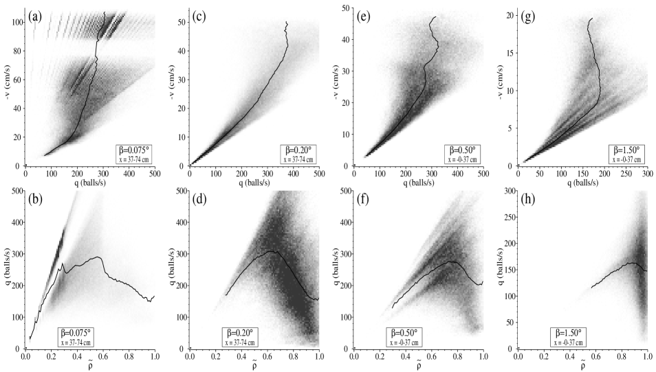
FIG. 22.: The $(q,v)$ and $(\rho,q)$ distributions for four different funnel angles: (a,b) $\beta=0.075^{\circ}$, (c,d) $\beta=0.20^{\circ}$, (e,f) $\beta=0.50^{\circ}$, (g,h) $\beta=1.50^{\circ}$. The solid lines are the averages, indicating the flow/speed diagram $v(q)$ or the fundamental diagram $q(\tilde{\rho})$ as appropriate.

For pipe flow ($\beta=0.075^{\circ}$) Fig. 22(a) shows a small queue region and then a large region similar to queue discharge behavior. In the fundamental diagram in Fig. 22(b) low densities dominate. The $q(\tilde{\rho})$ curve in (b) (solid line) has a parabolic shape which peaks at $\tilde{\rho}\sim 0.5$. The data set from which the distributions were derived contained only one shock wave, hence, certain regions contain no data since some flow states (e.g., $v\sim 80$ cm/s) simply did not occur during the measurement.

For intermittent flow ($\beta=0.2^{\circ}$) Fig. 22(c) displays a longer queue flow region than Fig. 22(a). It then changes smoothly into a relatively broader queue discharge region. The $(\tilde{\rho},q)$ distribution in Fig. 22(d) is dominated by moderately large densities ($\tilde{\rho}>0.5$) and $q(\tilde{\rho})$ peaks at a slightly higher value ($\tilde{\rho}\sim 0.7$) than pipe flow.

For the denser flows shown in Figs. 22(e) and (g), it becomes increasingly difficult to distinguish between queue flow and queue discharge. The queue discharge regions are found at lower values of $v$ and $q$, which is consistent with the general trend of falling average velocities (see Sec. VIII) and average flow rates ($q\sim\beta^{-0.4}$ for $\beta>0.5^{\circ}$[4]). The corresponding fundamental diagrams in Figs. 22(f) and (h) again have parabolic shapes which peak at increasingly higher densities ($\tilde{\rho}>0.8$). The shapes of the distributions close to $\tilde{\rho}=1$ are not very well-defined. We know from Secs. IV D and VIII that virtually all density variations are related to packing site effects at large $\beta$. Consequently, it should not be expected that the distribution for $\tilde{\rho}>0.9$ can be resolved. For $\tilde{\rho}<0.9$, the behavior in Fig. 22(h) is most likely caused by the manner in which the dense flow leaves the outlet.

In real traffic, shock waves are generally slower than vehicle speeds (see [15]) and the densities are low ($\tilde{\rho}<0.3$) during uncongested flow. These properties are similar to the flow conditions in true pipe flow ($\beta=0^{\circ}$), whereas our few measurements (of duration $\sim 8$ s) do not have the time and space resolution necessary to catch the full range of the shock dynamics. Thus we cannot display ball flow behavior corresponding to uncongested flow.

Flows for $\beta>0.2^{\circ}$ are strongly affected by packing sites and thus by the changing number of lanes as illustrated in Fig. 4. Several consecutive reductions in the number of lanes in traffic are seldom found, but a comparison would be interesting. A more general comparison between the manner in which granular shock waves and traffic jams propagate in space and time would also be interesting, but unfortunately there are practically no available $v(x,t)$ measurements in traffic with the appropriate temporal and spatial resolution.

X Summary

We have presented the results of particle tracking measurements on a two-dimensional flow of monodisperse balls. The circumstances of the creation and propagation of shock waves have been studied. In particular, we have observed how individual balls behave both in the shock region and between shocks, and established that the interaction of balls between shocks can be disregarded by a simple rescaling of gravity. The simultaneous tracking of thousands of balls has been used to study the time and space variations of quantities such as flow velocity, acceleration and granular temperature. This has been used to study the shock wave behavior in very dense flows, the processes surrounding the creation of new shocks, and the role played by granular temperature.

A Ball position determination

Each stored video frame is recalled from the harddisk as an array of unsigned 8-bit integers. This array is equivalent to a grey scale image where black corresponds to 0 and white to 255. Each frame is subtracted from the image of the empty funnel. Thus, the balls stand out as a white patch on a black background. We will call these patches ball images. Based on the local distributions of grey scale values, a threshold is determined. Everything above the threshold is defined as part of a ball. Areas of adjoining pixels with values over the threshold belong to the same ball. An estimate of the ball center position $(x_{c},y_{c})_{est}$ (based on a weighted average of the pixel values) and height (intensity in grey scale) is made. The height and estimated positions $(x_{c},y_{c})_{est}$ will be used as starting values in a fit of a ball’s image to a rotationally symmetric “bell-shaped” function representing it.

Next, we need to determine which pixels belong to the ball image and should be used in the fit. An area of pixels surrounding the estimated ball center $(x_{c},y_{c})_{est}$ is selected. Let $d$ be the distance from $(x_{c},y_{c})_{est}$ for each pixel and let $r$ be the ball radius. Pixels with $d\leq 0.9r$ are all selected. Pixels with $0.9r<d<1.45r$ are selected if the next pixels away from $(x_{c},y_{c})_{est}$ are not higher than the value of the pixel in question (if they are, it indicates that the value of the pixel is influenced by a wall or another ball). All other pixels are disregarded. In this way, most of the pixels belonging to the ball image and some of the surrounding black ones will be selected, while pixels belonging to other balls will be left out.

Typically, between 20 and 35 pixels are selected for the position fit of each ball. These pixel values are fitted to a rotationally symmetric bell-shaped function with 4 fitting parameters: peak height, $(x,y)$ components of the center position, and the ball radius. (The convergence of the fits is more stable when the radius is allowed to vary.) When a radial distribution of pixel values is found, the resulting curve matches the function $e^{-{|d|}^{3}}$ remarkably well, where $d$ is the pixel distance from $(x_{c},y_{c})$. In most fits, a bell-shaped function with a radial dependence $\sim e^{-{|d|}^{3}}$ also gives the best results. In a small number of fits ($<1\%$), however, a stable fit is not achieved with this function. In these cases a second fit is made with an ordinary Gaussian function $e^{-{|d|}^{2}}$ . The Gaussian fits give slightly inferior results on average but are much more stable in the “difficult” cases. All fits were made using the amoeba method [16]. At this point a table of ball center positions has been determined for each frame in the sequence.

The error of the ball center positions ($\lesssim 0.15$ mm) was determined in two ways. In the first, a number ($\sim 20$) of balls were glued to a rigid, transparent piece of plastic. This piece was translated and rotated in the funnel and a number of frames were shot. In each frame the relative positions of the balls should be constant and the noise level could subsequently be determined. In the second, individual balls were allowed to roll freely in the funnel (without touching the funnel walls or other balls). ¿From the smoothness of enlargements of the resulting trajectories, the noise level of the position detection could be estimated.

B Interference with pixel array of camera

In original versions of ball center position histograms of the type shown in Fig. 4, there were clear signs of horizontal stripe patterns where the distance between the stripes corresponded to the distance between neighboring lines of pixels in the camera. This indicated that there was some interference between the pixel periodicity of the camera and the determined ball center positions since there is no reason why some positions relative to the pixel array should occur significantly more often than others. Subsequent histograms of the fractions of the ball center positions in pixel coordinates were made. An example of such a histogram is shown in Fig. 23(a). These histograms confirmed the existence of interference along both the $x$ axis and the $y$ axis. For simplicity, we assume that this interference was the same in all areas of the camera and that this systematic remapping is “smooth”. With these assumptions it is relatively easy to map the positions back to their “true” values and thus eliminate the effect of this interference. The resulting repositionings of the ball centers are less than half the statistical uncertainty of the positions and thus it is of limited importance. In Fig. 23(b) a comparison is made between the same ball trajectory before and after the remapping. As can be seen, the effect is relatively small. The remapping has nevertheless been done for all data sets to avoid any “cumulative” effects of this systematic error. In Figs. 4(a,b) there is still a faint set of horizontal lines (with a vertical periodicity of $\sim 0.6$ mm) but this has been significantly reduced by the remapping.

FIG. 23.: (a) Distribution of fractional part of ball coordinates measured in pixel coordinates ($\beta=0.5^{\circ}$, $D=10$mm, $\theta=4.1^{\circ}$). (b) Comparison of $v_{y}$ for the same ball before and after re-mapping of ball coordinates. The “after re-mapping” curve is displaced $-2$ cm/s. ($\beta=0.15^{\circ}$, $D=10$mm, $\theta=4.1^{\circ}$). (The ball encounters a shock at $t=0.1$ s.)

C Assumption of transverse uniformity

Throughout this article the flow of balls has been treated as essentially one-dimensional. Since the width of the funnel ($\lesssim 10$ ball diameters) is relatively small compared with the other important length scales in the system (e.g., funnel length and shock separation), it is reasonable to assume that the flow is uniform across the funnel. Between shocks, balls essentially move independently of each other (see Sec. III C) and uniformity may be harder to maintain. In any case, this assumption should be checked. It is unfortunately hard to devise any meaningful statistics that could confirm the instantaneous transverse equilibrium of a moving shock wave. By averaging over $x$ and $t$ on the other hand, we can achieve meaningful statistics and subsequently check the $y/w(x)$ dependence of various flow properties. (When averaging over $x$ is done we must renormalize $y$ with $w(x)$ to make the averaging meaningful.)

FIG. 24.: The space and time averaged velocity profile versus $y/w(x)$ for different funnel angles ($D=10$ mm, $\theta=4.1^{\circ}$).

In Fig. 24 the $y/w$ dependence of $v$ is shown averaged over both $x$ (in 10 cm intervals) and $t$ for various flows. Both pipe flow and dense flow show flat velocity profiles while intermittent flow ($\beta=0.15^{\circ}$ and $\beta=0.3^{\circ}$) exhibits a drop near the funnel walls. This is not evidence of a shear flow situation. It simply means that between shocks (where high ball speeds occur) the regions are partially “statistically empty”, namely, when balls leave a shock, they uniformly occupy the full width of the funnel. The balls closest to the funnel walls will often collide with the wall and move towards the center of the funnel. In the middle part of the funnel they will collide with several other balls and in each collision the transverse energy will be reduced and the transverse momentum will be averaged out (since balls are coming from both walls). As a result the density will be somewhat higher in the middle of the funnel compared with regions close to the funnel walls. Thus, in the overall statistics, the fastest balls mostly contribute in the central part of the funnel. In pipe flow ($\beta=0^{\circ}$) this effect is not seen because the density is too low to eliminate transverse energy in the center of the funnel, since each ball basically follows its own “zig-zag” trajectory. (Note that the data for $\beta=0^{\circ}$ has been shifted downwards for clarity. The actual velocities are $\sim 120$ cm/s.) In dense flows ($\beta=0.6^{\circ}$ and $\beta=2.0^{\circ}$) the effect is not observed since the density is constantly high (see Figs. 19(c) and (e)) and there is no space for balls close to the funnel walls to move away as they accelerate following a shock.

REFERENCES

- [1] R. L. Brown and J. C. Richards, Principles of powder mechanics (Pergamon Press, Oxford, 1970); J. Lee, S. C. Cowin, and J. S. Templeton, Trans. Soc. Rheo. 18, 247 (1974); R. L. Michalowski, Powder Tech. 39, 29 (1984); G. W. Baxter, R. P. Behringer, T. Fagert, and G. A. Johnson, Phys. Rev. Lett. 62, 2825 (1989); A. A. Mills, S. Day, and S. Parkes, Eur. J. Phys. 17, 97 (1996). See also, R. P. Behringer and G. W. Baxter, eds., Pattern formation and complexity in granular flows (Springer-Verlag, 1993).
- [2] T. Pöschel, J. Phys. I France 4, 499 (1994); S. Horikawa, A. Nakahara, T. Nakayama, and M. Matsushita, J. Phys. Soc. Jap. 64, 1870 (1995); T. Raafat, J. P. Hulin, and H. J. Herrmann, Phys. Rev. E 53, 4345 (1996); O. Moriyama, N. Kuroiwa, M. Matsushita, and H. Hayakawa, Phys. Rev. Lett. 80, 2833 (1998).
- [3] K. L. Schick and A. A. Verveen, Nature 251, 599 (1974); X.-l. Wu, K. J. Måløy, A. Hansen, M. Ammi, and D. Bideau, Phys. Rev. Lett. 71, 9 (1993); C. T. Veje and P. Dimon, Phys. Rev. E 56, 4376 (1997); C. T. Veje, Ph.D. thesis, University of Copenhagen (1999).
- [4] C. T. Veje and P. Dimon, Phys. Rev. E 54, 4329 (1996); C. T. Veje, Master’s thesis, University of Copenhagen (1995).
- [5] S. Hørlück and P. Dimon, Phys. Rev. E 60, 671 (1999); S. Hørlück, Master’s thesis, University of Copenhagen (1997).
- [6] T. Le Pennec, M. Ammi, J. C. Messager, and A. Valance, Eur. Phys. J. B 7, 657 (1999).
- [7] T. G. Drake, J. Geophys. Res. 95, 8681 (1990); T. G. Drake, J. Fluid Mech. 225, 121 (1991).
- [8] S. Warr, G. T. H. Jacques, and G. M. Huntley, Powder Tech. 81, 41 (1994); S. Warr, G. M. Huntley, and G. T. H. Jacques, Phys. Rev. E 52, 5583 (1995).
- [9] D. H. Ballard and C. M. Brown, Computer vision (Prentice Hall, 1982).
- [10] S. Hørlück, preprint.
- [11] I. Goldhirsch and G. Zanetti, Phys. Rev. Lett. 70, 1619 (1993).
- [12] S. McNamara and W. R. Young, Phys. Rev. E 53, 5089 (1996).
- [13] See, for example, D. E. Wolf, M. Schrenkenberg, and A. Bachem, eds., Workshop on traffic and granular flow (World Scientific, Singapore, 1995).
- [14] M. J. Lighthill and G. B. Whitham, Proc. Roy. Soc. A 229, 317 (1955).
- [15] G. B. Whitham, Linear and nonlinear waves (Wiley, New York, 1974).
- [16] W. H. Press, S. A. Teukolsky, W. T. Vetterling, and B. P. Flannery, Numerical recipes in C: The art of scientific computing (Cambridge University Press, Cambridge, 1992).