Linked Cluster Series Expansions for Two-Particle Bound States

Abstract

We develop strong-coupling series expansion methods to study two-particle spectra of quantum lattice models. At the heart of the method lies the calculation of an effective Hamiltonian in the two-particle subspace. We explicitly consider an orthogonality transformation to generate this block diagonalization, and find that maintaining orthogonality is crucial for systems where the ground state and the two-particle subspace are characterized by identical quantum numbers. We discuss the solution of the two-particle Schrödinger equation by using a finite lattice approach in coordinate space or by an integral equation in momentum space. These methods allow us to precisely determine the low-lying excitation spectra of the models at hand, including all two-particle bound/antibound states. Further, we discuss how to generate series expansions for the dispersions of the bound/antibound states. These allow us to employ series extrapolation techniques, whereby binding energies can be determined even when the expansion parameters are not small. We apply the method to the (1+1)D transverse Ising model and the two-leg spin-$\frac{1}{/}2$ Heisenberg ladder. For the latter model, we also calculate the coherence lengths and determine the critical properties where bound states merge with the two-particle continuum.

I INTRODUCTION

The study of bound states and multiparticle excitations remains a challenging problem in many-body physics. Experimentally, there are several probes for low-dimensional magnetic or strongly correlated electronic systems which show spectral features associated with multiparticle continuum and bound states. These include two-magnon Raman spectra, optical absorption, photoemission and neutron scattering spectra. The multiparticle features often remain poorly understood. On the theoretical side, one example of the intriguing issues that may arise is the role that the increasing number of bound states play in the confinement-deconfinement transition in spin-Peierls systems. At the transition the spectrum switches from a soliton-antisoliton continuum to elementary triplet excitations, their bound states and continuum[4].

A controlled numerical framework for the calculation of multi-particle spectral properties, which can also account for various singularities as the coupling constants are varied, is currently missing. In one dimension, a variety of numerical methods including Lanczos, exact diagonalization and most notably density matrix renormalization group (DMRG) [5] hold promise for such calculations. However, unlike ground state and single-particle properties, the calculation of full dynamical properties like spectral functions still needs more conceptual advances. In higher than one dimension, all of these methods are restricted to small system sizes, which makes it difficult to study the thermodynamic limit.

On the other hand in the limits of weak or strong couplings, perturbation theory can be used to calculate all properties of the multiparticle spectra directly in the thermodynamic limit. If these calculations can be done to high orders, one can calculate multiparticle spectra in a systematic manner using extrapolation techniques even in cases where the perturbations are not weak. In principle, one can see that as the couplings are increased the number of bound states can change and states can come off or merge into the continuum. The resulting singularities should be amenable to series expansion methods.

In this paper, we show how to calculate multi-particle spectral properties from high-order perturbation expansions, using a linked cluster method. A brief outline and summary of the work was given in a recent letter[6]. Our method is quite distinct from the flow equation approach of Wegner[7], which has also been used recently by Uhrig and collaborators [8, 9] for the study of multiparticle spectral properties in one and two dimensions.

The linked cluster method is by far the most efficient way to generate perturbation series expansions for quantum Hamiltonian lattice models. For the ground state energy and related properties, a linked cluster approach was first discussed in unpublished work by Nickel[10], followed by work of Marland[11], Irving and Hamer[12] and others, as reviewed by He et al[13]. The approach was later rediscovered and applied to a whole new range of problems in condensed matter physics by Singh, Huse and Gelfand[14, 15].

For the energies of excited states, it is more difficult to formulate a true linked cluster expansion, although related methods have been known for some time[10, 16]. It was only in 1996 that the key to a true linked cluster expansion for one-particle excited states was discovered by Gelfand[17]. Since then, many applications of this technique have been made, calculating single-particle energies, dispersion relations and spectral functions in models of interest in condensed matter physics. For a recent review, see Gelfand and Singh[18].

The key advantage of the cluster expansion method is that the calculations can be carried out systematically and efficiently by fully automated computer programs. Furthermore, these methods work by breaking up the thermodynamic problem into a purely combinatorial problem and a number of finite-cluster problems. Thus, while they are technically harder in higher than one dimension, the difficulty is not fundamental. In fact, over the years, a number of workers[19, 20, 18, 21, 22] have independently developed efficient computer programs to generate these clusters automatically, and the cluster data up to quite high number of vertices for most 2-dimensional and 3-dimensional lattices including the simple-cubic, BCC and FCC lattices have been generated[19]: these data can be applied to a wide range of models.

At the heart of our new approach is a generalization of Gelfand’s linked cluster expansion for single-particle excited states to two-particle states. From a technical point of view, our most notable achievement is the development of an orthogonality transformation which leads to a linked cluster theorem for multi-particle states even when their quantum numbers are identical with the ground state. We show how to calculate energies and dispersion relations for two-particle excitations, and coherence lengths for the bound states. The further generalization to higher number of particle is then obvious in principle.

As a first check to ensure that the method is working correctly, we apply it to the case of the transverse Ising model in one dimension, which can be solved exactly in term of free fermions[23]. We show that the series for the 2-particle state agree with the exact results up to 12th order.

Finally, we apply the method to a non-trivial model, the 2-leg spin-$\frac{1}{/}2$ Heisenberg ladder, which has been much discussed recently[24, 25, 26, 27, 28, 29, 30, 31] as a prime example of a one-dimensional antiferromagnetic system with a gapped excitation spectrum. The two-particle bound states have already been studied by Damle and Sachdev[28] and Sushkov and Kotov[30, 31]. We perform a detailed study of these bound states, exhibiting in particular the characteristic features as each bound state emerges from the continuum.

In a companion paper[32], we apply the same techniques to a still more interesting case, the frustrated alternating Heisenberg chain, which displays the confinement-deconfinement transition discussed by Affleck[4].

The organization of the paper is as follows. Section II of the paper lays out the formalism and methods used to obtain the 2-particle spectra. Section III discusses the applications to the transverse Ising chain and the Heisenberg ladder, and Section IV summarizes our conclusions.

II FORMALISM

We consider a Hamiltonian

$$H=H_{0}+\lambda H_{1}\;,$$ (1)

where the unperturbed Hamiltonian $H_{0}$ is exactly solvable, and $\lambda$ is the perturbation parameter. In the lattice models of interest here, $H_{0}$ will typically consist of single-site operators, while interaction terms between different sites will be included in the perturbation operator $H_{1}$. The aim is to calculate perturbation series in $\lambda$ for the eigenvalues of $H$ and other quantities of interest. The calculation proceeds in three stages.

A Block Diagonalization

On any finite lattice or cluster of sites, the first step is to ‘block diagonalize’ the Hamiltonian to form an “effective Hamiltonian”, where the ground state sits in a block by itself, the 1-particle states form another block, the 2-particle states another block, and so on. Here a “particle” may refer to a lattice fermion, a spin-flip, or other excitation, depending on the model at hand. We assume that all the unperturbed states in each block are degenerate under $H_{0}$. There is no unique way to block diagonalize the Hamiltonian, but the eigenvalues and final results should be unique, independent of the method used, as long as the cluster expansion works correctly. Gelfand[17] used a similarity transform for this purpose:

$$H^{\rm eff}=O^{-1}HO\;.$$ (2)

This works correctly for most 1-particle problems, and also for those 2-particle states which have different quantum numbers to the ground state. However in general, especially for the 2-particle states which have identical quantum numbers to the ground state, we need to be a little more careful than this, in order to preserve all the proper symmetries of the Hamiltonian. We must ensure that the transformation is unitary. Here we will only consider the case when the Hamiltonian is real symmetric, and can be block diagonalized by an orthogonal transformation,

$$H^{\rm eff}=O^{T}HO$$ (3)

or more conveniently

$$OH^{\rm eff}=HO\;,$$ (4)

where

$$O^{T}=O^{-1}\;.$$ (5)

The orthogonality of O can be ensured by writing

$$O=e^{S}\;,$$ (6)

where S is real, antisymmetric

$$S^{T}=-S\;.$$ (7)

This transformation is constructed order-by-order in perturbation theory. The matrix elements of $H^{\rm eff}$ between different blocks are zero, up to the given order in perturbation theory. Each matrix is expanded in powers of $\lambda$:

$$O=\sum_{n=0}^{\infty}\lambda^{n}O^{n)}\;,$$ (8)

$$S=\sum_{n=0}^{\infty}\lambda^{n}S^{n)}\;,$$ (9)

$$H^{\rm eff}=\sum_{n=0}^{\infty}\lambda^{n}H_{\rm eff}^{n)}\;,$$ (10)

where at zeroth order we set

$$S^{0)}=0,\hskip 14.22636ptO^{0)}=I,\hskip 14.22636ptH_{\rm eff}^{0)}=H_{0}\;.$$ (11)

where $I$ is an unit matrix, $H_{0}$ is a diagonal matrix, with diagonal matrix elements $E_{i}^{0}$.

At higher orders $n\neq 0$, we have

$$O^{n)}=S^{n)}+\frac{1}{2}\sum_{m,l=1}^{n}S^{m)}S^{l)}\delta_{m+l,n}+\frac{1}{3!}\sum_{m,l,k=1}^{n}S^{m)}S^{l)}S^{k)}\delta_{m+l+k,n}+...$$ (12)

and

$$\sum^{n}_{m,l=0}O^{m)}H_{\rm eff}^{l)}\delta_{m+l,n}=H_{0}O^{n)}+H_{1}O^{n-1)}$$ (13)

and it is convenient to define

$$R^{n)}=O^{n)}-S^{n)}\;.$$ (14)

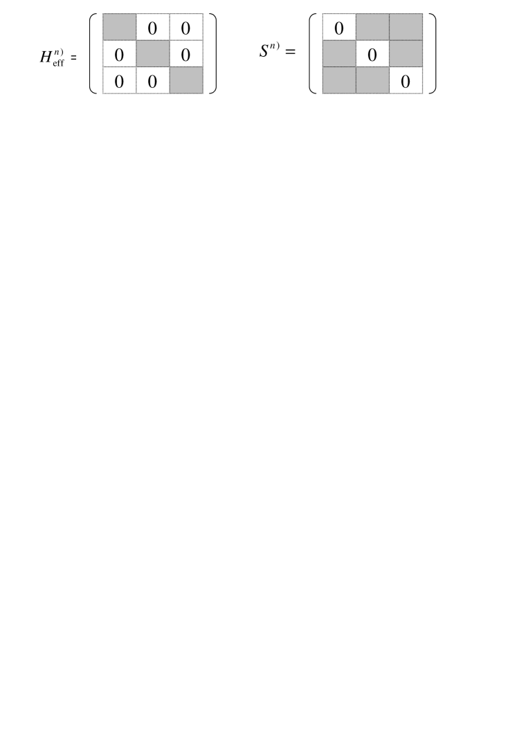
FIG. 1.: Block structure of the matrices $H^{n)}_{\rm eff}$ and $S^{n)}$. Setting the upper right blocks of $H^{n)}_{\rm eff}$ to zero determines the corresponding (shaded) blocks of $S^{n)}$; the diagonal blocks of $S^{n)}$ are set to zero.

If we demand that at any given order n the off-diagonal blocks of $H^{\rm eff}$ in (say) the upper right triangle vanish, then equations (13) determine the entries in the corresponding blocks of $S^{n)}$ (Figure 1). The transposed blocks in the lower left triangle are then determined by the antisymmetry condition (7); and only the diagonal blocks of $S$ remain to be determined. The simplest choice is to set the diagonal blocks to zero. Thus $S^{n)}$ is completely determined:

$$S^{n)}_{ij}=-R^{n)}_{ij}+\frac{1}{(E^{0}_{j}-E^{0}_{i})}\{H_{1}O^{n-1)}-\sum_{m,l=1}^{n-1}O^{m)}H^{l)}_{\rm eff}\delta_{m+l,n}\}_{ij}$$ (15)

or

$$O^{n)}_{ij}=\frac{1}{(E^{0}_{j}-E^{0}_{i})}\{H_{1}O^{n-1)}-\sum_{m,l=1}^{n-1}O^{m)}H^{l)}_{\rm eff}\delta_{m+l,n}\}_{ij}$$ (16)

for elements $ij$ in the off-diagonal (shaded) blocks. Then

$$(H^{n)}_{\rm eff})_{ij}=\{H_{1}O^{n-1)}-\sum_{m,l=1}^{n-1}O^{m)}H^{l)}_{\rm eff}\delta_{m+l,n}\}_{ij}$$ (17)

for elements in the diagonal blocks. The right-hand sides of equations (15,16,17) can all be computed from the results at order $(n-1)$.

The key differences here from the similarity transformation are as follows. In the similarity transformation, the diagonal blocks of $O^{n)}$ are undetermined, and so are chosen to be zero, while the off-diagonal blocks of $O^{n)}$ are antisymmetric and can be determined by demanding the off-diagonal blocks of $H^{n)}_{\rm eff}$ to be zero. In the orthogonal transformation, on the other hand, the diagonal blocks of $O^{n)}$ cannot be chosen to be zero. Instead the diagonal blocks of $S^{n)}$ are chosen to be zero, while the diagonal blocks of $O^{n)}$ are required to be nonzero by orthogonality, and are determined by Eq. (12).

At the end of this process, the effective Hamiltonian has been block diagonalized, up to a given order in perturbation theory. The orthogonal transformation will transform the unperturbed two-particle states into “dressed” states containing admixtures of different particle numbers; and in particular, there will be no annihilation process for these “dressed” states. The states will still be labelled by the positions of the original unperturbed particles; but now they will contain admixtures of other particle states at nearby locations.

At any finite order in perturbation theory, we may assume that the effective Hamiltonian will remain “local” (that is, interactions between states will not extend beyond a finite range); and will have the same bulk symmetries as the original Hamiltonian, such as translation symmetry. These properties are sufficient to admit a linked cluster approach to the calculation of eigenvalues.

We note that the solution of the equations above is not nearly as efficient as the similarity transformation of Gelfand: in particular, the solution of the equation (12) is expensive in CPU time and memory. In the Appendix, we discuss an alternative ‘2-block’ scheme which has the same efficiency as Gelfand’s; but which does not always allow a successful cluster expansion.

B Linked Cluster Expansions

Let us briefly summarize the linked cluster approach in various sectors.

1 Ground-state energy

The ground-state energy $E_{0}$ is a simple extensive quantity, and obeys the “cluster addition property”: if C is a cluster (or set of sites and bonds on the lattice) which is composed of two disconnected sub-clusters A and B, then

$$E_{0}^{C}=E_{0}^{A}+E_{0}^{B}\;.$$ (18)

Hence one finds[10, 11, 12, 13, 14, 15] that the ground-state energy per site for the bulk lattice can be expressed purely in terms of contributions from connected sub-clusters $\alpha$:

$$\epsilon_{0}=\sum_{\alpha}l_{\alpha}\epsilon_{\alpha}\;,$$ (19)

where $l_{\alpha}$ is the “lattice constant”, or number of ways per site that cluster $\alpha$ can be embedded in the bulk lattice, and $\epsilon_{\alpha}$ is the “proper energy” or “cumulant energy” for the cluster $\alpha$. In the language of Feynman diagrams, $\epsilon_{\alpha}$ can be thought of as the sum of all connected diagrams spanning the cluster $\alpha$[33].

A similar formula holds for the ground-state energy of any connected cluster $\alpha$ with open boundaries:

$$E_{0}^{\alpha}=\sum_{\beta}C_{\beta}^{\alpha}\epsilon_{\beta}\;,$$ (20)

where $C_{\beta}^{\alpha}$ is the embedding constant of the connected sub-cluster $\beta$ within cluster $\alpha$.

Equations (19) and (20) form the basis for a simple and efficient recursive algorithm to generate a perturbation series for $\epsilon_{0}$. The steps are:

• Generate a list of clusters $\alpha$, with their lattice constants $l_{\alpha}$ and embedding constants $C_{\beta}^{\alpha}$, appropriate to the problem at hand [21, 19, 20];

• For each cluster $\alpha$, the diagonal entry in the 0-particle sector of $H^{\rm eff}$ gives a perturbation series for the energy $E_{0}^{\alpha}$;

• Now invert equations (20) to solve for the cumulant energies $\epsilon_{\alpha}$, and substitute in (19) to obtain the desired perturbation series for $\epsilon_{0}$.

2 1-particle excited states

FIG. 2.: Decomposition of a 1-particle matrix element into irreducible components. The round box denotes the full matrix element, the square boxes the irreducible matrix elements, and the single line denotes a delta function.

Gelfand[17] discovered how to generalize the approach above to one-particle excited states. Let

$$E_{1}({\bf i,j})=\langle{\bf j}|H^{\rm eff}|{\bf i}\rangle$$ (21)

be the matrix element of $H^{\rm eff}$ between initial 1-particle state $|{\bf i}\rangle$ and final 1-particle state $|{\bf j}\rangle$, labelled according to their positions on the lattice. The excited state energy is not extensive, and does not obey the cluster addition property; but there is a related quantity which does. If cluster C is made up of disconnected sub-clusters A and B, and states $|{\bf i}\rangle$ and $|{\bf j}\rangle$ reside (say) on cluster A, then

$$E_{1}^{C}({\bf i,j})=E_{1}^{A}({\bf i,j})+E_{0}^{B}\;.$$ (22)

But if we define the “irreducible” 1-particle matrix element (Fig. 2)

$$\Delta_{1}({\bf i,j})=E_{1}({\bf i,j})-E_{0}\delta_{{\bf i,j}}\;,$$ (23)

then

$$\Delta_{1}^{C}({\bf i,j})=\Delta_{1}^{A}({\bf i,j})\;,$$ (24)

whereas if $|{\bf i}\rangle$ and $|{\bf j}\rangle$ reside on cluster B, then

$$\Delta_{1}^{C}({\bf i,j})=\Delta_{1}^{B}({\bf i,j})$$ (25)

or in general

$$\Delta_{1}^{C}({\bf i,j})=\Delta_{1}^{A}({\bf i,j})+\Delta_{1}^{B}({\bf i,j})\;,$$ (26)

where $\Delta_{1}({\bf i,j})$ vanishes for any cluster not containing i and j. Note that a 1-particle state cannot annihilate from one sub-cluster and reappear on the other, after the initial block diagonalization.

From the cluster addition property (26) it follows that the elements $\Delta_{1}({\bf i,j})$ can be expanded in terms of contributions from connected clusters alone, which are also “rooted”, or connected to the positions i and j. Hence they can be calculated efficiently by an algorithm like that of subsection (II B 1).

3 2-particle states

The generalization to two-particle states is now not hard to find. Let

$$E_{2}({\bf i,j;k,l})=\langle{\bf k,l}|H^{\rm eff}|{\bf i,j}\rangle$$ (27)

be the matrix element between initial 2-particle state $|{\bf i,j}\rangle$ and final state $|{\bf k,l}\rangle$. To obtain a quantity obeying the cluster addition property, we must subtract the ground-state energy and 1-particle contributions, to form the irreducible 2-particle matrix element [Fig. 3]:

$$\Delta_{2}({\bf i,j;k,l}) = E_{2}({\bf i,j;k,l})-E_{0}(\delta_{{\bf i,k}}\delta_{{\bf j,l}}+\delta_{{\bf i,l}}\delta_{{\bf j,k}})-\Delta_{1}({\bf i,k})\delta_{{\bf j,l}}-\Delta_{1}({\bf i,l})\delta_{{\bf j,k}}$$ (29)

$$-\Delta_{1}({\bf j,k})\delta_{{\bf i,l}}-\Delta_{1}({\bf j,l})\delta_{{\bf i,k}}\;.$$

This quantity is easily found to be zero for any cluster unless i, j, k and l are all included in that cluster, and it obeys the cluster addition property. Once again, the block diagonalization ensures that two particles cannot “annihilate” from one cluster and “reappear” on another disconnected one. Thus the matrix elements of $\Delta_{2}$ can be expanded in terms of connected clusters alone, which are rooted or connected to all four positions i, j, k, l.

FIG. 3.: Decomposition of two identical particle matrix element into irreducible components. Notation as in Fig. 2.

C Calculation of eigenvalues

For the ground state energy, a perturbation series for the eigenvalue was already obtained at the end of subsection II B 1. For the excited state sectors, some further work is required.

1 1-particle states

A perturbation series for the dispersion relation of the 1-particle states can be calculated by a Fourier transform. Translation invariance implies that

$$\Delta_{1}({\bf i,j})\equiv\Delta_{1}({\bf\delta})\;,$$ (30)

where ${\bf\delta}$ is the difference between positions i and j; and that the 1-particle states are eigenstates of momentum:

$$|{\bf K}\rangle=\frac{1}{\sqrt{N}}\sum_{{\bf j}}\exp(i{\bf K\cdot j})|{\bf j}\rangle\;,$$ (31)

(where $N$ is the number of sites in the lattice), with energy gap

$$\omega_{1}({\bf K})=\sum_{{\bf\delta}}\Delta_{1}({\bf\delta})\cos({\bf K\cdot\delta})\;.$$ (32)

Here we have assumed that $\Delta_{1}({\bf\delta})$ is reflection symmetric, so that

$$\Delta_{1}({\bf-\delta})=\Delta_{1}({\bf\delta})\;.$$ (33)

2 2-particle states

The calculation of the eigenvalues in this case is a little more involved than in the 1-particle case. We follow the procedure of Mattis[34].

Consider an unsymmetrized state of non-identical particles, types $a$ and $b$. Then there are $N(N-1)$ states on an $N$-site lattice, labelled by positions $|{\bf i,j}\rangle$, where i,j refer to the positions of particles $a$ and $b$, respectively. We have assumed here that two particles may not reside at the same position (the results are easily amended if this is not the case). Then the irreducible 2-particle matrix element is:

$$\Delta_{2}^{ab}({\bf i,j;k,l}) = E_{2}^{ab}({\bf i,j;k,l})$$ (35)

$$-E_{0}\delta_{{\bf i,k}}\delta_{{\bf j,l}}-\Delta_{1}^{a}({\bf i,k})\delta_{{\bf j,l}}-\Delta_{1}^{b}({\bf j,l})\delta_{{\bf i,k}}\;.$$

Let the 2-particle eigenstate be:

$$|\psi\rangle=\sum_{{\bf i,j}}f_{{\bf ij}}|{\bf i,j}\rangle,\hskip 8.53581pt(i\neq j)\;,$$ (36)

substitute in the Schrödinger equation

$$H^{\rm eff}|\psi\rangle=E|\psi\rangle$$ (37)

and take the overlap with $\langle{\bf i,j}|$, then one obtains:

$$(E-E_{0})f_{{\bf ij}}-\sum_{{\bf k\neq j}}\Delta^{a}_{1}({\bf k,i})f_{{\bf kj}}-\sum_{{\bf k\neq i}}\Delta^{b}_{1}({\bf k,j})f_{{\bf ik}}=\sum_{{\bf k,l}}\Delta^{ab}_{2}({\bf k,l;i,j})f_{{\bf kl}}\;,\hskip 5.69054pt({\bf i\neq j})\;.$$ (38)

Completing the sums on the left-hand side, one obtains:

$$(E-E_{0})f_{{\bf ij}}-\sum_{\bf k}[\Delta^{a}_{1}({\bf k,i})f_{{\bf kj}}+\Delta^{b}_{1}({\bf k,j})f_{{\bf ik}}] = \sum_{{\bf k,l}}\Delta^{a,b}_{2}({\bf k,l;i,j})f_{{\bf kl}}$$ (40)

$$-\Delta^{a}_{1}({\bf j,i})f_{{\bf jj}}-\Delta^{b}_{1}({\bf i,j})f_{{\bf ii}}\;,$$

The fictitious amplitudes $f_{{\bf ii}}$ are introduced to simplify the calculations, and are taken to be defined by these equations[34].

Now define a centre-of-mass position co-ordinate

$${\bf R}=\frac{1}{4}({\bf i+j+k+l})\;,$$ (41)

and relative co-ordinates

$${\bf r}=\frac{1}{2}({\bf i+j-k-l})\;,$$ (42)

$$\delta_{1}={\bf i-j}\;,$$ (43)

$$\delta_{2}={\bf k-l}\;.$$ (44)

Translation invariance then implies that

$$\Delta_{2}({\bf i,j;k,l})\equiv\Delta_{2}({\bf r,\delta_{1},\delta_{2}})\;.$$ (45)

Next, perform a Fourier transformation,

$$f({\bf K,q})=\frac{1}{N}\sum_{{\bf i,j}}e^{i({\bf k_{1}\cdot i+k_{2}\cdot j})}f_{{\bf ij}}\;,$$ (46)

where ${\bf K,q}$ are the centre-of-mass and relative momenta:

$${\bf K}=({\bf k}_{1}+{\bf k}_{2})\;,$$ (47)

$${\bf q}=\frac{1}{2}({\bf k}_{1}-{\bf k}_{2})\;,$$ (48)

then equation (40) leads to

$$[E-E_{0}-\sum_{{\bf\delta}}[\Delta^{a}_{1}({\bf\delta})\cos({\bf K\cdot\delta}/2+{\bf q\cdot\delta})+\Delta^{b}_{1}({\bf\delta})\cos({\bf K\cdot\delta}/2-{\bf q\cdot\delta})]f({\bf K,q}) =$$ (49)

$$\frac{1}{N}\sum_{{\bf q^{\prime}}}f({\bf K,q^{\prime}})[\sum_{{\bf r,\delta_{1},\delta_{2}}}\Delta^{ab}_{2}({\bf r,\delta_{1},\delta_{2}})\cos({\bf K\cdot r}+{\bf q\cdot\delta_{1}}-{\bf q^{\prime}\cdot\delta_{2}})$$ (50)

$$-\sum_{{\bf\delta}}\Delta^{a}_{1}(\delta)\cos({\bf K\cdot\delta}/2+{\bf q\cdot\delta})+\Delta^{b}_{1}(\delta)\cos({\bf K\cdot\delta}/2-{\bf q\cdot\delta})]\;,$$ (51)

where we have again assumed reflection symmetry

$$\Delta^{a,b}_{1}(\delta)=\Delta^{a,b}_{1}(-\delta)\;,$$ (52)

$$\Delta^{ab}_{2}({\bf r,\delta_{1},\delta_{2}})=\Delta^{ab}_{2}({\bf-r,-\delta_{1},-\delta_{2}})\;.$$ (53)

Finally, look for solutions with definite exchange symmetry.

Symmetric states

$$f_{ij}=+f_{ji}$$ (54)

therefore

$$f({\bf K,q})=+f({\bf K,-q})\;.$$ (55)

‘Averaging’ over $f({\bf K,\pm q})$ (i.e. taking $\frac{1}{2}[f({\bf K,q})+f({\bf K,-q})]$), we get:

$$\{E-E_{0}-\sum_{{\bf\delta}}[\Delta^{a}_{1}({\bf\delta})+\Delta^{b}_{1}({\bf\delta})]\cos({\bf K\cdot\delta/2})\cos({\bf q\cdot\delta})\}f({\bf K,q}) =$$ (56)

$$\frac{1}{N}\sum_{{\bf q^{\prime}}}f({\bf K,q^{\prime}})[\sum_{{\bf r,\delta_{1},\delta_{2}}}\Delta^{ab}_{2}({\bf r,\delta_{1},\delta_{2}})\cos({\bf K\cdot r})\cos({\bf q\cdot\delta_{1}})\cos({\bf q^{\prime}\cdot\delta_{2}})$$ (57)

$$-\sum_{{\bf\delta}}[\Delta^{a}_{1}(\delta)+\Delta^{b}_{1}(\delta)]\cos({\bf K\cdot\delta}/2)\cos({\bf q\cdot\delta})]\;.$$ (58)

Antisymmetric states

$$f_{ij}=-f_{ji}$$ (59)

therefore

$$f({\bf K,q})=-f({\bf K,-q})\;.$$ (60)

‘Averaging’ over $f({\bf K,\pm q})$ (i.e. taking $\frac{1}{2}[f({\bf K,q})-f({\bf K,-q})]$), we get:

$$\{E-E_{0}-\sum_{{\bf\delta}}[\Delta^{a}_{1}({\bf\delta})+\Delta^{b}_{1}({\bf\delta})]\cos({\bf K\cdot\delta/2})\cos({\bf q\cdot\delta})\}f({\bf K,q}) =$$ (61)

$$\frac{1}{N}\sum_{{\bf q^{\prime}}}f({\bf K,q^{\prime}})\sum_{{\bf r,\delta_{1},\delta_{2}}}\Delta^{ab}_{2}({\bf r,\delta_{1},\delta_{2}})\cos({\bf K\cdot r})\sin({\bf q\cdot\delta_{1}})\sin({\bf q^{\prime}\cdot\delta_{2}})\;.$$ (62)

Identical particles

If the particles $a$ and $b$ are identical, the solution is the same as for symmetric states except the labels $a$ and $b$ must now be dropped, and to avoid double counting it turns out that the $\Delta_{2}$ term must be multiplied by an extra factor of 1/2:

$$[E-E_{0}-2\sum_{{\bf\delta}}\Delta_{1}({\bf\delta})\cos({\bf K\cdot\delta}/2)\cos({\bf q\cdot\delta})]f({\bf K,q}) =$$ (63)

$$\frac{1}{N}\sum_{{\bf q^{\prime}}}f({\bf K,q^{\prime}})[\frac{1}{2}\sum_{{\bf r,\delta_{1},\delta_{2}}}\Delta_{2}({\bf r,\delta_{1},\delta_{2}})\cos({\bf K\cdot r})\cos({\bf q\cdot\delta_{1}})\cos({\bf q^{\prime}\cdot\delta_{2}})$$ (64)

$$-2\sum_{{\bf\delta}}\Delta_{1}(\delta)\cos({\bf K\cdot\delta}/2)\cos({\bf q\cdot\delta})]\;.$$ (65)

The above integral equations can be solved, for a given value of ${\bf K}$, using standard discretization techniques. Instead of using continous momentum ${\bf q}$, one can use $N$ discretized and equally spaced values of momentum, so that instead of solving the complicated integral equation, one only needs to compute the eigenvalue and eigenvector of an $N\times N$ matrix for the discretized system. Notice that the matrix is nonsymmetric due to the unphysical $f_{ii}$ term we have introduced in Eq. (40), but even so the eigenvalues obtained from this matrix are real. The solutions we obtain also include an unphysical one with eigenvalue equal to 0 (this is also due to the unphysical $f_{ii}$ term). The results obtained from the calculation with discretized momenta will converge to those with continous momentum as $N\to\infty$. Actually for those bound states with finite coherence length, the calculation will normally be well converged for quite small values of $N$, but for unbound states, we have an infinite coherence length, so one may need to do finite $N$ extrapolations to get results at $N=\infty$.

There are two methods to compute the eigenvalues of the matrix for the discretized system. Obviously one can get numerical results for the eigenvalues, for a given value of coupling $\lambda$ and momentum ${\bf K}$, via standard numerical techniques where we just perform a naive sum for the series in $\Delta_{1}$ and $\Delta_{2}$. The results presented in a preceding Letter [6] are based on this method; but then one cannot carry out a series extrapolation, and so one may not be able to reach a region of critical coupling. A better technique is to compute the series in $\lambda$ for the eigenvalues through degenerate perturbation theory: that is, by explicit diagonalization of the matrix within the degenerate subspace, order by order in perturbation theory, and then one can perform a series extrapolation. The problem with this method is that the series does not always exist, for example for those bound states appearing at some nonzero value of $\lambda$.

The two particle continuum is delimited by the maximum (minimum) energy of two single particle excitations whose combined momentum is the center of mass momentum. Apart from the unphysical eigenvalue, there may be multiple solutions above/below the two-particle continuum. Those solutions with energy below the bottom edge of the continuum are the bound states, while the solutions with energy higher than the upper edge of the continuum are the antibound states. The binding energy is defined as the energy difference between the lower edge of the continuum and the energy of the bound state, while the antibinding energy is defined as the energy difference between the upper edge of continuum and the energy of an antibound state.

Note that the series for $\Delta_{2}$ may depend on the transformation used to block diagonalize the Hamiltonian. If we compute $\Delta_{2}$ (and also $\Delta_{1}$) to order $n$, the resulting series for the 2-particle energy obtained from the above integral equation will have two parts: the part up to order $n$ is independent of the transformation, while the higher order terms are incomplete, and may depend on the transformation. The numerical solution of the integral equation may also depend partly on the transformation, since it contains the higher order term. Also note that the series for $\Delta_{2}$ need not have any singularities. The singularities, if they exist, arise in the solution of the Schrödinger equation, so our method should be able to explore new bound states arising as we vary the momentum ${\bf K}$. If we get a numerical solution, rather than a series solution, to the Schrödinger equation, we should also be able to explore new bound states arising as we increase $\lambda$ as long as the naive sum to the series converges.

D Finite Lattice Approach

Once the cluster expansions for the irreducible matrix elements $\Delta_{1}$ and $\Delta_{2}$ have been developed, the Schrödinger equation in the two-particle subspace can be solved by an alternative method that works in coordinate space rather than momentum space. By restricting to a finite but large system with periodic boundary conditions, the two-particle Schrödinger equation becomes a finite-dimensional matrix of equations. The cluster expansion results provide the matrix elements of the effective Hamiltonian as a power series in the expansion parameter. The centre of mass momentum is a conserved quantity, thus, for a given value of the centre of mass momentum, one is left with a Schrödinger equation in the separation variable. One can truncate the perturbation theory at a given order and solve the Schrödinger equation numerically. One can then vary the size of the system, which only increases the dimension of matrix to be diagonalized linearly, to study convergence. We have frequently used this method to compare with and check the momentum-space discretization solutions.

This ‘finite lattice approach’ also allows us to obtain power series expansions for bound state energies, by a non-degenerate perturbation theory, provided the bound state exists “localized” in the limit $\lambda\to 0$. For those “extended” bound states in the limit $\lambda\to 0$[32], one still needs to do degenerate perturbation theory, just as in the case of the momentum-space discretization solutions. Another advantage of this method over the the momentum-space discretization technique is that the matrix one deals with is always symmetric.

Furthermore, it gives us explicit real-space wave functions, from which the coherence length and other properties can be deduced. The coherence length $L$ is defined by

$$L={\sum_{{\bf r}}|{\bf r}|f_{{\bf r}}^{2}\over\sum_{{\bf r}}f_{{\bf r}}^{2}}$$ (66)

where $f_{{\bf r}}$ is the amplitude (the eigenvector) for two single-particle excitations separated by distance ${\bf r}$.

III RESULTS

We apply the new method to the (1+1)D transverse Ising model and a two-leg spin-$\frac{1}{/}2$ Heisenberg ladder.

A Transverse Ising model

In order to verify that our new technique is giving the correct results, we firstly apply it to a simple model, the $S=\frac{1}{/}2$ transverse Ising model in (1+1)-dimensions, which is exactly solvable in terms of free fermions. The Hamiltonian for it reads

$$H=\sum_{i}(1-\sigma^{z}_{i})-\lambda\sum_{i}\sigma^{x}_{i}\sigma^{x}_{i+1}\;,$$ (67)

Here we take the first term as the unperturbed Hamiltonian $H_{0}$, and the second term as the perturbation $H_{1}$. The ground state of $H_{0}$ is the unique state with all spins pointing up. The lowest excited states (1-particle excitations) for $H_{0}$ flip one of the spin from spin up to spin down. The exact result[23] for the 1-particle dispersion relation is

$$E_{1}(q)=2\sqrt{1+\lambda^{2}-2\lambda\cos q}\;.$$ (68)

For the 2-particle excitations, the unperturbed states have two spins down. Since this model can be mapped into free fermions, there are no 2-particle bound states, and the 2-particle excitation energy is simply the sum of two 1-particle dispersions, that is

$$E_{2}(q_{1},q_{2})=2\sqrt{1+\lambda^{2}-2\lambda\cos q_{1}}+2\sqrt{1+\lambda^{2}-2\lambda\cos q_{2}}\;,$$ (69)

where $q_{1}$ and $q_{2}$ are the momenta of each particle. Note that this is a non-trivial example for our method as the similarity transformation does not even lead to a cluster expansion.

We have implemented the algorithm described above for this model. For the 1-particle excitation, we can easily reproduce the exact results through the different block diagonalization schemes mentioned before. For the 2-particle excitations, although there are no bound states, the terms $\Delta_{2}$ are not zero. That is because we are using the spin representation; in a fermion representation, the $\Delta_{2}$ would be expected to vanish. We have computed them to order $\lambda^{12}$ by using the 2-block method. The series coefficients up to order $\lambda^{6}$ are given[35] in Table I. With these series, one can solve the discretized version of the integral equation to get the binding and antibinding energy for any given value of momentum $k$ and coupling $\lambda$. Our results show that for all $k$ and $\lambda$, the binding/antibinding energy scales as $1/N^{2}$, and approaches to zero as $N\to\infty$: this is consistent with the absence of bound/antibound states in this model. The results for $\lambda=0.5$ and $k=0,\pi/2,\pi$ are shown in Fig. 4. We have also checked that the resulting series for $E_{2}$ agrees with (69) for the lowest and highest energy of 2-particle states up to 12th order, and the coherence length is infinity, as expected.

FIG. 4.: The binding energy (full points) and antibinding energy (open points) $E_{b}$ versus $1/N^{2}$ ($N$ is the size of the matrix) for the transverse Ising model with coupling $\lambda=0.5$ and momentum $k=0$ (dotted lines), $\pi/2$ (dashed lines), $\pi$ (solid lines).

B Heisenberg ladder

The second model we have investigated is the 2-leg spin-$\frac{1}{2}$ Heisenberg ladder, where the Hamiltonian is

$$H=\sum_{i}\{J_{\perp}{\bf S}_{i}\cdot{\bf S}^{\prime}_{i}+J[{\bf S}_{i}\cdot{\bf S}_{i+1}+{\bf S}_{i}^{\prime}\cdot{\bf S}^{\prime}_{i+1}]\}\;,$$ (70)

where ${\bf S}_{i}$ (${\bf S}^{\prime}_{i}$) denotes the spin at site $i$ of the first (second) chain. $J$ is the interaction between nearest-neighbor spins along the chain, and $J_{\perp}$ is the interaction between nearest-neighbor spins along the rungs. In the present paper the intra-chain coupling is taken to be antiferromagnetic (that is, $J_{\perp}>0$ ) whereas the interchain coupling $J$ can be either antiferromagnetic or ferromagnetic.

The antiferromagnetic Heisenberg ladder has attracted a good deal of attention recently [24, 25, 26, 27, 28, 29, 30, 31]. It is of experimental interest in that there are a number of quasi-one-dimensional compounds which may be described by the model [24]. It is also a prime example of a one-dimensional antiferromagnetic system with a gapped excitation spectrum. Damle and Sachdev [28] as well as Sushkov and Kotov [30] have shown that the system exhibits two-particle bound states, one singlet and one triplet. Our aim here is to explore the properties of these bound states more closely.

In the dimer limit $J/J_{\perp}=0$, the ground state is the product state with the spins on each rung forming a spin singlet. The first excited state consists of a spin triplet excitation on one of the rungs. As $J/J_{\perp}$ increases, this state evolves smoothly, and the system has a gapped excitation spectrum[25, 26, 27]. The dimer expansions have been computed previously up to order $(J/J_{\perp})^{23}$ for the ground-state energy and up to order $(J/J_{\perp})^{13}$ for the 1-particle triplet excitation spectrum[26]. The occurrence of two-particle bound states in this model has been shown by first-order strong-coupling expansions [28, 29] as well as a leading order calculation using the analytic Brueckner approach[30, 31].

FIG. 5.: The excitation spectrum for the Heisenberg spin ladder at $J/J_{\perp}=0.2$. Beside the two-particle continuum (gray shaded), there are three massive quasiparticles: a singlet bound state (S), a triplet bound state (T) below the continuum and a quintet antibound state (Q) above the continuum.

FIG. 6.: The binding/antibinding energy $E_{b}/J_{\perp}$ (upper window) and the rescaled binding/antibinding energy $E_{b}/J_{\perp}(k-k_{c})^{2}$ (lower window) for the Heisenberg spin ladder at $J/J_{\perp}=0.2$.

Here we have calculated series for the dispersions of the 2-particle bound states up to order $(J/J_{\perp})^{7}$ for the singlet bound state ($S$), and to order $(J/J_{\perp})^{12}$ for the triplet bound state ($T$) and the quintet antibound state ($Q$). The reason why the singlet series is computed to only 7th order compared to 12th order for the triplet and quintet states is that the singlet has the same quantum numbers as the ground state. Thus a much more elaborate orthogonalization method is required to implement the cluster expansion for the singlet. For the triplet and quintet bound states, we can use the similarity transformation or the 2-block orthogonal transformation to implement the cluster expansion. Up to order $(J/J_{\perp})^{3}$, the dispersion for the singlet bound state ($E_{S}/J_{\perp}$), triplet bound state ($E_{T}/J_{\perp}$), quintet antibound state ($E_{Q}/J_{\perp}$) are

$$E_{S}/J_{\perp} = 2-\frac{3\,x}{2}+\frac{19\,x^{2}}{16}+\frac{9\,x^{3}}{32}+\left(-\frac{x}{2}+\frac{x^{2}}{8}-\frac{51\,x^{3}}{128}\right)\,\cos(k)$$ (73)

$$+\left(-\frac{5\,x^{2}}{16}-\frac{21\,x^{3}}{32}\right)\,\cos(2\,k)-\frac{37\,x^{3}\,\cos(3\,k)}{128}+O(x^{4})\;,$$

$$E_{T}/J_{\perp} = 2-\frac{3\,x}{2}+\frac{11\,x^{2}}{8}+\frac{17\,x^{3}}{16}+\left(-x-\frac{x^{2}}{4}+\frac{9\,x^{3}}{16}\right)\,\cos(k)$$ (75)

$$+\left(-\frac{x^{2}}{2}-\frac{x^{3}}{2}\right)\,\cos(2\,k)-\frac{5\,x^{3}\,\cos(3\,k)}{16}+O(x^{4})\;,$$

$$E_{Q}/J_{\perp} = 2+\frac{3\,x}{2}+\frac{11\,x^{2}}{8}-\frac{3\,x^{3}}{16}+\left(x-\frac{x^{2}}{4}-\frac{27\,x^{3}}{16}\right)\,\cos(k)$$ (77)

$$+\left(-\frac{x^{2}}{2}-\frac{3\,x^{3}}{8}\right)\,\cos(2\,k)+\frac{7\,x^{3}\,\cos(3\,k)}{16}+O(x^{4})\;,$$

where $x\equiv J/J_{\perp}$. The full dispersion series for the singlet state, and the series for the energy gap at $k=\pi$ for singlet, triplet and quintet bound/antibound states and the lower edge and upper edge of continuum are listed in Table II and III; the other series are available upon request[35]. Figs. 5 and 6 show the dispersion and the binding/antibinding energy at $J/J_{\perp}=0.2$ for the two-particle continuum as well as the the two-particle bound/antibound states. Here we can see there is a singlet ($S=0$) and a triplet ($S=1$) bound state of two elementary triplets below the two-particle continuum, and a quintet ($S=2$) antibound state above the continuum.

From these graphs, we can also see that these bound/antibound states exist only when the momentum $k$ is larger than some “critical momentum” $k_{c}$: the series in Eq. (6) and Table II are valid only for $k\geq k_{c}$. It is interesting to explore the behaviour of the binding energies near this critical momentum. From the series for the one-particle and two-particle dispersions, one can get leading order results for $k_{c}$ as

$$k_{c}=\left\{\begin{array}[]{ll}\sqrt{10x}+O(x)&\mbox{$S=0$}\\ 2\pi/3-5x/(2\sqrt{3})-109x^{2}/(48\sqrt{3})+O(x^{3})&\mbox{$S=1$}\\ 2\pi/3+5x/(2\sqrt{3})+47x^{2}/(48\sqrt{3})+O(x^{3})&\mbox{$S=2$}\end{array}\right.$$ (78)

and in the limit $k\to k_{c}$, the behaviour of the binding energy is

$$E_{b}/J = (k-k_{c})^{2}[5x/8+975x^{2}/128+O(x^{3})]$$ (80)

$$+(k-k_{c})^{3}[12+115x+O(x^{2})]\sqrt{10x}/192+O[(k-k_{c})^{4}]$$

for the singlet bound state, and

$$E_{b}/J = (k-k_{c})^{2}[3/8-x/32+0.45313x^{2}+O(x^{3})]$$ (82)

$$+(k-k_{c})^{3}[\sqrt{3}/16-53x/(64\sqrt{3})+0.19245x^{2}+O(x^{3})]+O[(k-k_{c})^{4}]$$

for the triplet bound state. For the quintet antibound state, the antibinding energy is

$$E_{b}/J = (k-k_{c})^{2}[3/8+x/32-0.40625x^{2}+O(x^{3})]$$ (84)

$$+(k-k_{c})^{3}[\sqrt{3}/16+53x/(64\sqrt{3})+1.00886x^{2}+O(x^{3})]+O[(k-k_{c})^{4}]\;.$$

Here one can see that for all bound/antibound states the “critical index” is 2, independent of the order of expansion, so one expects that this is exact.

FIG. 7.: The critical $(J_{/}J_{\perp})_{c}$ versus $k$ for singlet (S), triplet (T) and quintet (Q) bound/antibound states of the Heisenberg ladder. The solid lines with errorbars are the results obtained from Dlog Padé approximants to the series for binding/antibinding energy $E_{b}$ for given $k$, while the dotted lines are the results of Eq. (78).

A better way to locate the critical line in the $(J/J_{\perp})$-$k$ plane is to calculate the Dlog Padé approximants to the series for the binding/antibinding energy at a fixed momentum $k$. For those critical points lying at $x_{c}<0.2$, the resulting critical point and critical index are very accurate, correct up to 5 digits, and again one finds the critical index is exactly 2. The results for the triplet bound state at $k=3\pi/5$ are given in Table IV. The results for the critical points are given in Fig. 7, together with the results from Eq. (78). From this figure, one can see that as $J/J_{\perp}\to\infty$, $k_{c}$ for the singlet and triplet bound states approaches the same value, about $0.4\pi$, while $k_{c}$ for the quintet antibound state approaches $\pi$. To demonstrate that $E_{b}$ is proportional to $(k-k_{c})^{2}$ near $k_{c}$, we also plot in Fig. 5 the results for $E_{b}/J_{\perp}(k-k_{c})^{2}$ at $J/J_{\perp}=0.2$.

The binding/antibinding energy at $k=\pi$ for bound/antibound states versus $J/J_{\perp}$ is plotted in Fig. 8. In the limit $J/J_{\perp}\to 0$, $E_{b}/J_{\perp}$ is proportional to $J/J_{\perp}$, so in the figure we plot $E_{b}/J$ versus $J/J_{\perp}$. We can see that as $J/J_{\perp}$ increases, $E_{b}/J$ for the singlet bound state firstly increases, passes through a maximum at about $J/J_{\perp}=0.4$, then decreases, while $E_{b}/J$ for the triplet bound state and the quintet antibound state decreases monotonically. At $J/J_{\perp}=1/2$, we find the binding/antibinding energies at $k=\pi$ for the singlet, triplet, and quintet bound/antibound states are $E_{b}/J=$1.03(3), 0.385(1) and 0.0855(5), respectively. The binding energy for the singlet bound state is substantially larger than the value 0.70 obtained in [31].

FIG. 8.: The binding/antibinding energy $E_{b}$ at $k=\pi$ versus $J/J_{\perp}$ for singlet ($S$), triplet ($T$) and quintet (Q) bound/antibound states of the Heisenberg ladder. Several different integrated differential approximants to the series are shown.

FIG. 9.: The coherence length $L$ versus momentum $k$ for singlet (S), triplet (T) and quintet (Q) bound/antibound states of the Heisenberg ladder at $J/J_{\perp}=0.2$.

We have also computed the coherence length $L$ for these bound/antibound states. The results for $J/J_{\perp}=0.2$ are shown in Fig. 9, where we find that $L$ diverges as $1/(k-k_{c})$ as $k$ approaches $k_{c}$. This is to be expected, as the state becomes unbound at that point. The coherence length at $k=\pi$ versus $J/J_{\perp}$ is shown in Fig. 10, where we can see that at $J=0$, $L=1$. This is as expected, as the formation of these bound states is due to the attraction of two triplets on neighboring sites. As $J/J_{\perp}$ increases, the coherence length $L$ increases slowly. $L$ for the quintet antibound state is larger than that for the triplet bound state, which is larger than for the singlet bound state.

FIG. 10.: The coherence length $L$ versus $J/J_{\perp}$ at $k=\pi$ for singlet (S), triplet (T) and quintet (Q) bound/antibound states of the Heisenberg ladder.

IV Conclusions

In conclusion, we have developed new strong-coupling expansion methods to study two-particle spectra of quantum lattice models. We described in full detail the block diagonalization of the Hamiltonian, order by order in perturbation theory, to construct an effective Hamiltonian in the two-particle subspace. This work is closely related to Gelfand’s prior work on using similarity transformations to obtain an effective Hamiltonian for the single-particle subspace [17]. We found that one needs to define a two-particle irreducible matrix element, for a cluster expansion to exist. Furthermore, one needs to maintain explicit orthogonality in the transformations in order to study the two-particle subspace characterized by identical quantum numbers to the ground state. An example of the latter is the two-particle singlet excitation sector in dimerized spin models.

We have discussed the solution of the integral equation one obtains by a Fourier transformation of the two-particle Schrödinger equation and by a ‘finite-lattice approach’. These allow us to precisely determine the low-lying excitation spectra of the models at hand, including all two-particle bound/antibound states. Furthermore, we have shown that one can generate series expansions directly for the dispersions of the bound/antibound states, provided these bound states exist in the limit $\lambda\to 0$. These allow us to apply series extrapolation techniques such as Dlog Padés and differential approximants to study binding energies even when the perturbation parameter is not small.

We applied the method to the (1+1)D transverse Ising model and the two-leg spin-$\frac{1}{/}2$ Heisenberg ladder. While the first model does not include any bound states, we find a singlet and a triplet bound state in the latter model as well as a quintet antibound state. We generated explicit expressions for the dispersions of these states as series in the exchange couplings. Further, we have determined the critical momenta $k_{c}$, where these additional massive quasi-particles merge with the two-particle continuum, which are non-zero for all three states. The explicit expressions of the binding energies at the respective critical momenta are found to contribute first in order $(k-k_{c})^{2}$, independent of the order of the strong coupling expansion. We computed the coherence length for these states and find that the coherence length diverges as one approaches the critical momentum where these states become unbound.

There are several possible direction for future research along these lines. Of course there are many different models to which these methods might be applied. In particular, it remains to show that the linked cluster expansion works sucessfully for two or higher dimensional models. One would also like to know how to calculate other quantities associated with multipartcle excitations, such as spectral weights, lifetimes, and scattering S-matrices. The latter would provide a handle on some important dynamical properties of the system.

A 2-Block Approach

There is an alternative way to perform the block diagonalization of Section II A, which is almost as efficient as Gelfand’s similarity transformation. The idea is to separate the effective Hamiltonian into only two blocks, one containing the states in the sector of interest (e.g. the 1-particle states, or the 2-particle states), and the other containing all other states. One can prove in this two-block approach that $O^{n)}$ determined in this way is antisymmetric with respect to the off-diagonal blocks, and symmetric with respect to the diagonal blocks. Rather than use the complicated equation (12), one can then determine the diagonal blocks of $O^{n)}$ in a much more efficient way by the orthogonality condition (5) which can be rewritten in the following form:

$$\{O^{n)}+O^{n)T}\}_{ij}=-\sum_{m=1}^{n-1}\{O^{m)}O^{n-m)T}\}_{ij}$$ (A1)

for elements in the diagonal blocks. Thus one can dispense with the matrix $S$, and work with $O$ only.

Unfortunately, although it is more efficient, this approach does not always seem to allow a successful cluster expansion. The reason for this is not understood at the present time.

TABLE I.: Series coefficients for $\Delta_{2}(r,\delta_{1},\delta_{2})=\sum_{k}\Delta_{2}^{k}(r,\delta_{1},\delta_{2})x^{k}$ in the (1+1)D transverse Ising model, obtained by the 2-block method. Nonzero coefficients $\Delta_{2}^{k}(r,\delta_{1},\delta_{2})$ up to order $k=6$ are listed.

$(k,2r,\delta_{1},\delta_{2})$	$\Delta_{2}^{k}(r,\delta_{1},\delta_{2})/4$	$(k,2r,\delta_{1},\delta_{2})$	$\Delta_{2}^{k}(r,\delta_{1},\delta_{2})/4$	$(k,2r,\delta_{1},\delta_{2})$	$\Delta_{2}^{k}(r,\delta_{1},\delta_{2})/4$	$(k,2r,\delta_{1},\delta_{2})$	$\Delta_{2}^{k}(r,\delta_{1},\delta_{2})/4$
( 2,-2, 1, 1)	5.000000$\times 10^{-1}$	( 4, 4, 2, 2)	1.562500$\times 10^{-1}$	( 5,-5, 3, 2)	1.093750$\times 10^{-1}$	( 6, 4, 3, 1)	$-$5.468750$\times 10^{-2}$
( 2, 2, 1, 1)	5.000000$\times 10^{-1}$	( 4,-4, 3, 1)	1.562500$\times 10^{-1}$	( 5, 5, 3, 2)	1.093750$\times 10^{-1}$	( 6,-6, 1, 5)	8.203125$\times 10^{-2}$
( 3,-3, 1, 2)	2.500000$\times 10^{-1}$	( 4, 4, 3, 1)	1.562500$\times 10^{-1}$	( 5,-5, 4, 1)	1.093750$\times 10^{-1}$	( 6, 6, 1, 5)	8.203125$\times 10^{-2}$
( 3, 3, 1, 2)	2.500000$\times 10^{-1}$	( 5,-3, 1, 2)	$-$7.812500$\times 10^{-2}$	( 5, 5, 4, 1)	1.093750$\times 10^{-1}$	( 6,-6, 2, 4)	8.203125$\times 10^{-2}$
( 3,-3, 2, 1)	2.500000$\times 10^{-1}$	( 5, 3, 1, 2)	$-$7.812500$\times 10^{-2}$	( 6,-2, 1, 1)	$-$1.953125$\times 10^{-2}$	( 6, 6, 2, 4)	8.203125$\times 10^{-2}$
( 3, 3, 2, 1)	2.500000$\times 10^{-1}$	( 5,-3, 2, 1)	$-$7.812500$\times 10^{-2}$	( 6, 2, 1, 1)	$-$1.953125$\times 10^{-2}$	( 6,-6, 3, 3)	8.203125$\times 10^{-2}$
( 4,-2, 1, 1)	$-$1.250000$\times 10^{-1}$	( 5, 3, 2, 1)	$-$7.812500$\times 10^{-2}$	( 6,-4, 1, 3)	$-$5.468750$\times 10^{-2}$	( 6, 6, 3, 3)	8.203125$\times 10^{-2}$
( 4, 2, 1, 1)	$-$1.250000$\times 10^{-1}$	( 5,-5, 1, 4)	1.093750$\times 10^{-1}$	( 6, 4, 1, 3)	$-$5.468750$\times 10^{-2}$	( 6,-6, 4, 2)	8.203125$\times 10^{-2}$
( 4,-4, 1, 3)	1.562500$\times 10^{-1}$	( 5, 5, 1, 4)	1.093750$\times 10^{-1}$	( 6,-4, 2, 2)	$-$5.468750$\times 10^{-2}$	( 6, 6, 4, 2)	8.203125$\times 10^{-2}$
( 4, 4, 1, 3)	1.562500$\times 10^{-1}$	( 5,-5, 2, 3)	1.093750$\times 10^{-1}$	( 6, 4, 2, 2)	$-$5.468750$\times 10^{-2}$	( 6,-6, 5, 1)	8.203125$\times 10^{-2}$
( 4,-4, 2, 2)	1.562500$\times 10^{-1}$	( 5, 5, 2, 3)	1.093750$\times 10^{-1}$	( 6,-4, 3, 1)	$-$5.468750$\times 10^{-2}$	( 6, 6, 5, 1)	8.203125$\times 10^{-2}$

TABLE II.: Series coefficients for the dispersion $E(k)/J_{\perp}=\sum_{k,n}a_{k,n}x^{k}\cos(nk)$ for the singlet bound state of the Heisenberg ladder. Nonzero coefficients $a_{k,n}$ up to order $k=7$ are listed. Note that the series are valid only for $k\geq k_{c}$.

(k,n)	$a_{k,n}$	(k,n)	$a_{k,n}$	(k,n)	$a_{k,n}$	(k,n)	$a_{k,n}$
( 0, 0)	2.0000000	( 2, 1)	1.2500000$\times 10^{-1}$	( 5, 2)	$-$3.9255371	( 5, 4)	$-$1.5305176
( 1, 0)	$-$1.5000000	( 3, 1)	$-$3.9843750$\times 10^{-1}$	( 6, 2)	$-$1.0420853$\times 10^{1}$	( 6, 4)	$-$5.0236816
( 2, 0)	1.1875000	( 4, 1)	$-$1.9453125	( 7, 2)	$-$2.8697990$\times 10^{1}$	( 7, 4)	$-$1.5335112$\times 10^{1}$
( 3, 0)	2.8125000$\times 10^{-1}$	( 5, 1)	$-$5.2039795	( 3, 3)	$-$2.8906250$\times 10^{-1}$	( 5, 5)	$-$3.8916016$\times 10^{-1}$
( 4, 0)	$-$1.2919922	( 6, 1)	$-$1.2828888$\times 10^{1}$	( 4, 3)	$-$1.0078125	( 6, 5)	$-$2.3588257
( 5, 0)	$-$3.4462891	( 7, 1)	$-$3.3050570$\times 10^{1}$	( 5, 3)	$-$2.7506104	( 7, 5)	$-$9.1123085
( 6, 0)	$-$7.1851196	( 2, 2)	$-$3.1250000$\times 10^{-1}$	( 6, 3)	$-$7.5901184	( 6, 6)	$-$5.0462341$\times 10^{-1}$
( 7, 0)	$-$1.6790197$\times 10^{1}$	( 3, 2)	$-$6.5625000$\times 10^{-1}$	( 7, 3)	$-$2.2107023$\times 10^{1}$	( 7, 6)	$-$3.6886940
( 1, 1)	$-$5.0000000$\times 10^{-1}$	( 4, 2)	$-$1.5449219	( 4, 4)	$-$3.1933594$\times 10^{-1}$	( 7, 7)	$-$6.8294907$\times 10^{-1}$

TABLE III.: Series coefficients for dimer expansions of the energy gap $E/J_{\perp}$ of singlet bound state, triplet bound state, quintet antibound state, and the lower and upper edge of the continuum at $k=\pi$ for the the Heisenberg ladder. Coefficients of $(J/J_{\perp})^{n}$ up to order $n=12$ are listed.

$n$	singlet bound state	triplet bound state	quintet antibound state	lower edge of continuum	upper edge of continuum
0	2.000000000	2.000000000	2.000000000	2.000000000	2.000000000
1	$-$1.000000000	$-$0.500000000	0.500000000	0.000000000	0.000000000
2	0.750000000	1.125000000	1.125000000	1.000000000	2.000000000
3	0.312500000	0.312500000	0.687500000	0.250000000	1.250000000
4	$-$0.203125000	$-$0.476562500	0.148437500	$-$0.625000000	$-$0.500000000
5	$-$0.558593750	$-$0.742187500	$-$0.242187500	$-$1.031250000	$-$1.843750000
6	$-$0.356445313	$-$0.399414063	$-$0.198242188	$-$0.595703125	$-$1.119140625
7	0.440856934	0.444519043	0.219665527	0.648925781	1.613769531
8		1.282394409	0.294692993	1.615997314	3.436676025
9		0.964994431	$-$0.865842819	1.012023926	1.011138916
10		$-$1.139695843	$-$3.052285552	$-$1.200890859	$-$4.719360987
11		$-$3.099767812	$-$3.914894695	$-$2.788565993	$-$6.971628388
12		$-$1.480682586	0.070329791	$-$0.814231584	0.478638977

TABLE IV.: The critical point (pole) and critical index (residue) obtained from $[n/m]$ Dlog Padé approximants to the series for the binding energy at $k=3\pi/5$ for the triplet bound state of the Heisenberg ladder. An asterisk denotes a defective approximant.

n	$[(n-2)/n]$	$[(n-1)/n]$	$[n/n]$	$[(n+1)/n]$	$[(n+2)/n]$
	pole (residue)	pole (residue)	pole (residue)	pole (residue)	pole (residue)
n= 2		0.13342(2.100484)	0.13067(1.917138)∗	0.13163(1.993828)	0.13173(2.002998)
n= 3	0.13169(1.999149)	0.13172(2.001628)	0.13170(2.000083)	0.13170(2.000146)	0.13170(1.999905)
n= 4	0.13171(2.000658)	0.13170(2.000143)	0.13170(2.000097)	0.13170(1.999987)	0.13170(1.999999)
n= 5	0.13170(1.999826)∗	0.13170(1.999969)	0.13170(1.999997)
n= 6	0.13170(2.000016)

REFERENCES

- [1] Email address: w.zheng@unsw.edu.au
- [2] Email address: c.hamer@unsw.edu.au
- [3] Present address: Bell Labs, Lucent Technologies, Murray Hill, NJ 07974
- [4] I. Affleck, in Dynamical Properties of Unconventional Magnetic Systems (NATO ASI, Geilo, Norway, 1997).
- [5] T. D. Kühner and S. R. White, Phys. Rev. B 60, 335 (1999).
- [6] S. Trebst, H. Monien, C. J. Hamer, W. H. Zheng and R. R. P. Singh, to appear in Phys. Rev. Lett. 85, (2000).
- [7] F. Wegner, Ann. Phys. (Leipzig) 3, 77 (1994); C. Knetter and G. S. Uhrig, Eur. Phys. J. B 13, 209 (2000).
- [8] G. S. Uhrig and B. Normand, Phys. Rev. B 58, R14705 (1998).
- [9] C. Knetter, E. Müller-Hartmann and G. S. Uhrig, J. Phys. Condens. Matter 12, 9069 (2000).
- [10] B. G. Nickel, unpublished.
- [11] L. G. Marland, J. Phys. A14, 2047 (1981).
- [12] A. C. Irving and C. J. Hamer, Nucl. Phys. B230, 361 (1984).
- [13] H-X. He, C. J. Hamer and J. Oitmaa, J. Phys. A23, 1775 (1990).
- [14] R. R. P. Singh, M. P. Gelfand and D. A. Huse, Phys. Rev. Lett. 61, 2484 (1988).
- [15] M. P. Gelfand, R. R. P. Singh and D. A. Huse, J. Stat. Phys. 59, 1093 (1990).
- [16] C. J. Hamer and A. C. Irving, J. Phys. A17, 1649 (1984).
- [17] M. P. Gelfand, Solid State Comm. 98, 11 (1996).
- [18] M. P. Gelfand and R. R. P. Singh, Advances in Physics 49, 93 (2000).
- [19] Jaan Oitmaa has developed some efficient computer programs to generate a wide range of cluster for various lattices.
-
[20]
Recently some of the authors (ST and HM) have been using object oriented
programming techniques to represent the graph theoretical part of the problem.
For more information see
http://cond-mat.uni-bonn.de/ClusterExpansion. - [21] See e.g. J. L. Martin, in “Phase Transitions and Critical Phenomena”, vol. 3, p. 47 (ed. C. Domb and M. S. Green, Academic, New York, 1973).
- [22] D.C. Rapaport, Comp. Phys. Commun. 8, 320(1974).
- [23] P. Pfeuty, Ann. Phys. (New York), 57, 79 (1970).
- [24] For a review, see E. Dagotto and T. M. Rice, Science 271, 618 (1996).
- [25] S. Gopalan, T. M. Rice, and M. Sigrist, Phys. Rev. B 49, 8901 (1994).
- [26] J. Oitmaa, R. R. P. Singh, and W.H. Zheng, Phys. Rev. B 54, 1009 (1996); W. H. Zheng, V. Kotov, and J. Oitmaa, Phys. Rev. B 57, 11439 (1998).
- [27] R. Eder, Phys. Rev. B 57, 12832 (1998).
- [28] K. Damle and S. Sachdev, Phys. Rev. B 57, 8307 (1998).
- [29] C. Jurecka and W. Brenig, Phys. Rev. B 61, 14307 (2000).
- [30] O. P. Sushkov and V. N. Kotov, Phys. Rev. Lett. 81, 1941 (1998).
- [31] V. N. Kotov, O. P. Sushkov, and R. Eder, Phys. Rev. B 59, 6266 (1999).
- [32] W. H. Zheng C. J. Hamer, R. R. P. Singh, S. Trebst, and H. Monien, cond-mat/0010243, to be published.
- [33] C. J. Hamer and A. C. Irving, Nucl. Phys. B230, 336 (1984).
- [34] D. C. Mattis, “The Theory of Magnetism I”, p. 146 (Springer-Verlag, New York, 1981).
- [35] Explicit results for the series will be made available electronically at http://www.phys.unsw.edu.au/~zwh.