Stability analysis of static solutions in a Josephson junction

Abstract

We present all the possible solutions of a Josephson junction with bias current and magnetic field with both inline and overlap geometry, and examine their stability. We follow the bifurcation of new solutions as we increase the junction length. The analytical results in terms of elliptic functions in the case of inline geometry, are in agreement with the numerical calculations and explain the strong hysteretic phenomena typically seen in the calculation of the maximum tunneling current. This suggests a different experimental approach based on the use, instead of the external magnetic field the modulus of the elliptic function or the related quantity the total magnetic flux to avoid hysteretic behavior and unfold the overlapping $I_{max}(H)$ curves.

I Introduction

The static properties of a narrow Josephson junction are well characterized by the static sine-Gordon equation [1]. They are experimentally measured by the maximum tunneling current $I_{max}$ as a function of the external field $H$. This is an important and useful measurement since it is required not only for the characterization of the junction properties but also to tailor a device with the desired maximum current. In contrast to its simple form, the static sine–Gordon differential equation problem poses several mathematical and computational challenges. The complete analysis of all of its solutions is hard due to various interesting properties (nonlinearity, non definiteness, periodicity, boundary conditions of Newmann type) inherent to the sine-Gordon problem and the determination of $I_{max}$ either theoretically, numerically or experimentally is difficult.

Several studies analyzing the dynamic and static stability of fluxons in the sine-Gordon equation have appeared in the literature in the past two decades with [2, 3, 4, 5] being the most representative of them. All these studies combine theoretical and numerical analysis and they mainly address the case where there is no external current or magnetic field applied on the junction. None of the above studies is comprehensive enough as far as exploiting all solutions and studying the affect of all physical and geometrical parameters of the problem.

The main objective of this study is fourfold.

• To analytically express all static solutions of 1-dimensional narrow Josephson junctions in a way that will allow us to examine their stability properties and their evolution with respect to the size of the junction, and the applied magnetic field and current.

• To explain the hysteretic behavior and if possible to find the important physical parameters that unravel the hysterisis.

• To build a numerical simulation framework that will allow us to verify some of our theoretical results and show that they apply to more complicated Josephson junction configurations.

• To propose an experimental procedure that will enable us to examine the properties of superconducting devices in a more accurate way. This approach is particularly useful for the analysis of devices that deviate from the standard mathematical model currently used i.e. junctions with impurities, inhomogeneities, …

We should mark here that, at the present, a complete theoretical analysis of such devices is not feasible while numerical simulations, based on state-of-the-art software packages [6, 7], usually fail to capture all the important features. This is mainly due to the difficulty to track the continuation branches and to deal with the bifurcation points involved. It is worth to mark here that the effects of the above mentioned difficulties are clearly seen, even in a relatively simple case, by the fact that it was only very recently [5] realized that the critical value of the bias current corresponds not to a termination point, as conjectured for many years, but to a turning point in the bifurcation diagram.

In addition to the above, the experimental analysis and the computer simulation and analysis of superconducting devices modeled by the sine-Gordon equation require an initial guess that is reasonably close to the desired solution. The selection of such initial guesses significantly affects the effectiveness of the various continuation methods needed to determine $I_{max}$. These guesses will be extensions of the various 1-D solutions obtained here. Therefore the results of the present study are expected to be fully utilized in effectively analyzing two dimensional window Josephson junctions.

The behavior of a Josephson junction is determined by the Josephson characteristic length $\lambda_{J}$ which depends both on material and geometry properties. For a short junction of length $l\ll\lambda_{J}$ the $I_{max}$ vs $H$ pattern (shown in Fig. 1a for normalized length $w=\frac{l}{\lambda_{J}}=1.0$) presents the usual Fraunhoffer pattern

$$I_{max}=\frac{sin\pi\frac{\Phi}{\Phi_{0}}}{\pi\frac{\Phi}{\Phi_{0}}},$$

where $\Phi=Hld$ is the applied flux, $\Phi_{0}=\frac{\hbar}{2e}$ the flux quantum and $d$ the magnetic thickness [1]. Each of the lobes in the diagram can be labeled by the pair of integers $(n,n+1)$ where at one end the magnetic field corresponds to exactly $n$ fluxons (i.e. flux= $n\Phi_{0}$) and at the other end $n+1$ fluxons. For the case of a long junction the problem was solved by Owen and Scalapino [8], and there, the different lobes overlap (as shown in Fig. 1b for $w=10$).

It should be remarked that the sine-Gordon equation, due to its nonlinearity and periodicity with several equilibrium points, has a multiplicity of solutions as shown by the overlapping lobes (in Fig. 1b) and the existence of several unstable branches which play an important role in the hysteretic behavior as you vary the external magnetic field. The unstable branches are of interest too because one can stabilize them, by introducing small defects, and therefore they should lead to observable maximum current. As we will see later in the discussion a defect can modify significantly the relative amplitude of the different lobes in the $I_{max}~{}~{}{\rm vs}~{}~{}H$ curve. The unstable branches can be partially traced experimentally if we perform a quasistatic scanning of the magnetic field.

The rest of the paper is organized as following. In section 2 we present the mathematical problem, give the explicit analytical solutions using elliptic functions and sketch the stability analysis. In section 3 we study the solutions in the particular case of zero magnetic field $H=0$, and in section 4 the analytic solutions for zero current $I=0$. We study both theoretically and numerically their stability in section 5 and we calculate the maximum tunneling current. In section 6 we briefly propose an experimental procedure which utilizes our numerical procedure. We summarize our results in the last section.

II Inline Geometry and Stability of Solutions

The case of inline geometry is a one dimensional problem, even for a wide junction, and one can obtain analytic solutions [8]. Furthermore one can easily check their stability by using linear perturbations. The particular cases of zero external magnetic field and inline bias current also reduce the overlap boundary conditions to inline ones. In the 1-dimensional case we have to solve the following problem

$$-\frac{d^{2}{\Phi}(x,t)}{dt^{2}}+\frac{d^{2}{\Phi}(x,t)}{dx^{2}}=\sin{\Phi}(x,t),~{}~{}~{}$$ (1)

with the inline boundary condition

$$\frac{d{\Phi}}{dx}\left|{}_{x=\pm{w}/2}\right.=\pm\frac{{I}}{2}+H\equiv\gamma_{\pm},~{}~{}~{}~{}$$ (2)

where $w$ is the normalized junction length and ${I}$ is the current line density.

Eq. (1) has a static solution $\Phi_{0}(x)$, implicitly expressed using elliptic functions [9] as

$$\sin\Phi_{0}(x)=-2\sqrt{m}~{}sn\left(x+x_{0}|m\right)~{}dn\left(x+x_{0}|m\right),~{}~{}~{}~{}$$ (3)

$$\cos\Phi_{0}(x)=2{m}~{}sn^{2}\left(x+x_{0}|m\right)-1,~{}~{}~{}~{}~{}$$ (4)

$$\frac{d\Phi_{0}}{dx}=2\sqrt{m}~{}cn\left(x+x_{0}|m\right),~{}~{}~{}$$ (5)

where the modulus $m$ determines the period of the $cn$ elliptic function (equal to $4K(m)$) and the arbitrary constant $x_{0}$ the phase at the center of the junction. They are determined by the boundary conditions (2). Introducing (5) into (2) we get

$$~{}~{}~{}~{}~{}~{}~{}~{}~{}~{}~{}~{}2\sqrt{m}~{}cn(x_{0}+\frac{w}{2}|m)=\gamma_{+},~{}~{}~{}$$ (6)

$$~{}~{}~{}~{}~{}~{}~{}~{}~{}~{}~{}~{}2\sqrt{m}~{}cn(x_{0}-\frac{w}{2}|m)=\gamma_{-}.~{}~{}~{}$$ (7)

A useful quantity to classify the solutions is the fluxon content or the magnetic flux in units of the quantum of flux, defined by

$$N_{f}=\frac{1}{2\pi}\left\{\Phi(\frac{w}{2})-\Phi(-\frac{w}{2})\right\}.$$

At specific values of $H$, $N_{f}$ takes integer values, so that the flux is that of an integer number of fluxons.

To check the stability of the static solution (3)-(5) we consider small perturbations on the static solution $\Phi_{0}(x)$ in the form

$$\Phi(x,t)=\Phi_{0}(x)+U(x,t)~{}~{}~{}~{}~{}~{}~{}~{}$$ (8)

and linearize Eq. (1) with respect to $U(x,t)$, to obtain

$$-U_{tt}+U_{xx}=\cos\Phi_{0}(x)\cdot U.~{}~{}~{}~{}~{}~{}~{}~{}$$ (9)

There is no loss of generality if we consider specific perturbations in the form

$$U(x,t)=X(x)e^{st}.~{}~{}~{}~{}~{}~{}$$ (10)

This way we obtain from Eq. (9) the eigenvalue equation

$$-X^{\prime\prime}+\cos\Phi_{0}(x)\cdot X=\lambda\cdot X,$$ (11)

under the boundary conditions

$$X^{\prime}|_{x=\pm w/2}=0.~{}~{}~{}~{}~{}~{}~{}$$ (12)

In Eq. (11) $\lambda=-s^{2}$. It is seen from Eq. (10) that if the eigenvalue problem (11)-(12) has a negative eigenvalue the static solution $\Phi_{0}(x)$ is unstable. If all the eigenvalues are positive $\Phi_{0}(x)$ is stable, while the case $\lambda=0$ corresponds to neutral stability and defines the boundary of stability. In the following we consider the two special cases $\gamma_{+}=\gamma_{-}~{}(I=0)$ and $\gamma_{+}=-\gamma_{-}~{}(H=0)$ separately, since the associated boundary conditions are easy to handle and the stability analysis is simplified.

To get a feeling concerning the possible solutions, we plot from the boundary conditions (2) and (6,7) the constant $H$ and $I$ contours in the plane of the $m$ and $x_{0}$ parameters in Fig. 2. We give different plots for $m<1$ and $m>1$. The lines labeled with ”$0$” correspond to $H=0$ (or $I=0$ for $I$ contours) and in both cases their network encloses areas with a single maximum (denoted by ”$+$”) or minimum (”$-$”) inside. Notice that there are two types of curves on which $H=0$ (or $I=0$) as summarized in Table  I.

The curved lines in Fig. 2 correspond to the solutions of the first line in the table which we call fixed $x_{0}$ solutions, in the sense that the shift is a fixed fraction of the period. From (6,7) we see that the physical quantities $I$ and $H$ are periodic functions of $x_{0}$ with period $4K(m)$. There are also solutions that have a fixed $m=m^{\star}$ and arbitrary $x_{0}$, and correspond to the vertical lines in Fig. 2 (remark that contour fitting can be distorted when two equicurrent lines cross). Similar results hold for the constant $I$ contours. For $m>1$ at the vertical $I=0$ curves we have an integer number of fluxons in the junction. Thus on the lines through $c$ ($a$) we have $N_{f}=1$ (2) correspondingly. In the current contours the points $f$ and $b$ correspond to peaks in the $I_{max}$ (see section 4.4). In the following we will focus our attention on the solutions where either $H$ or $I$ .

III No magnetic field case (H=0)

In the absence of external magnetic field we have $\gamma_{+}=-\gamma_{-}=\frac{I}{2}$ and Eqs. (6,7) reduce to

$$~{}~{}~{}2\sqrt{m}cn\left(x_{0}+\frac{w}{2}|m\right)=\frac{I}{2},~{}~{}~{}$$ (13)

$$\sqrt{m}cn\left(x_{0}-\frac{w}{2}|m\right)=-\frac{I}{2},~{}~{}~{}$$ (14)

which determine the parameters $m$ and $x_{0}$ that characterize the periodicity and phase shift of the static solutions. There are two different classes of solutions due to the antisymmetry of the boundary conditions, which can be satisfied for different $I$ either by fixing $x_{0}$ or $m$.

A Fixed $x_{0}$ solutions

It is seen from Eqs. (13,14) and the symmetry of the elliptic functions that for positive $I$ one choice for $x_{0}$ in (13,14) is $x_{0}=-K(m)$ ($K(m)$ is the elliptic integral of the first kind), so that $x_{0}$ is fixed to $\frac{1}{4}$ of the period of the elliptic function. It is in that sense that we call them fixed $x_{0}$ solutions. Strictly $x_{0}$ is not a constant independent of $m$ since $K(m)$ is a function of $m$. Thus we have (see [9])

$$\frac{I}{2}=2\sqrt{m(1-m)}~{}\frac{sn(\frac{w}{2}|m)}{dn(\frac{w}{2}|m)},~{}~{}~{}0\leq m<1,\,\,\,~{}~{}~{}$$ (15)

$$\cos\Phi_{0}(x)=2~{}m~{}\frac{cn^{2}(x|m)}{dn^{2}(x|m)}-1,~{}~{}~{}0\leq m<1,\,\,\,~{}~{}~{}$$ (16)

$$\sin\Phi_{0}(x)=2~{}\sqrt{m~{}(1-m)}\frac{cn(x|m)}{dn^{2}(x|m)},~{}~{}~{}0\leq m<1.\,\,\,$$ (17)

Another possibility is $x_{0}=K(m)$ ($x_{0}$ is shifted by half of a period) for the case that $2K(m)<\frac{w}{2}<4K(m)$, or more generally when $sn(\frac{w}{2}|m)<0$, since we are limiting ourselves to $I>0$. This means that every time $w$ increases by $2\pi$ we introduce two extra solutions. To put it in other words the function $I(m)$, in (15), is highly oscillating for large $w$. We do not need to consider the case that $m>1$ since in that case we cannot satisfy the antisymmetric boundary conditions for the external current.

In Fig. 3a we present three plots of ${I}$ vs $m$ for $w=\frac{2\pi}{3},\,\,\,\frac{3\pi}{2},\,\,\,\frac{5\pi}{2}$. We see that for small $w<2\pi$ there is, as expected, only one lobe for $x_{0}=-K(m)$, and as we will see later only the part to the right of the maximum will correspond to stable solutions, while the peak corresponds to the maximum current for zero magnetic field. For $w=\frac{5\pi}{2}$ we have an extra lobe, with the left one at $x_{0}=K(m)$ and the right at $x_{0}=-K(m)$. For $w=10$ (dashed line in Fig. 3b) the right lobe has a maximum within $10^{-3}$ of $m=1$ and corresponds to $x_{0}=K(m)$, while the left to $x_{0}=-K(m)$. The jump in path along two different curves is necessary because of the restriction of positive current $I$. Of course the curve is symmetric about the $I=0$ line. The right lobe for $w=10$ is shown in the inset of Fig. 3b in expanded form (solid line) with a different scale for $m$. The part that is of experimental interest is the last lobe near $m=1$ to the right of the maximum. The two extremal $m$ values correspond to trivial solutions $\Phi_{0}(x)=\pi~{}(m=0)$ and $\Phi_{0}(x)=0~{}(m=1)$, the first of which is clearly unstable (pendulum analogy) and the second is stable. For currents above zero at $w=10$ there are four possible solutions for a given $I<I^{\star}$, where $I^{\star}$ is the maximum of the lowest lobe.

Because the last lobe for large $w$ is very steep it is useful to give some analytic formulas valid near $m=1$ and for the maximum point. By using asymptotic formulas and assuming that $m_{1}\equiv 1-m\approx\epsilon^{2}$, where $\epsilon$ is a small parameter, we obtain the value of $m_{1}$ where $I$ is a maximum as

$$m_{1}^{max}=\frac{4}{\sinh^{2}\frac{w}{2}}.$$

The result is consistent with our scaling assumption with

$$\frac{1}{\sinh\frac{w}{2}}\sin\epsilon.$$

Thus care is required when simplifying the analytic formulas in [9] (see p. 574). The corresponding maximum current is

$$I=4-\frac{8}{\sinh^{2}\frac{w}{2}},$$ (18)

so that for large junction length $w$ it approaches exponentially the infinite length limit. To the right of the maximum the relation between $I(m_{1})$ is

$$I=4-m_{1}^{3/2}\frac{\tanh\frac{w}{2}}{{\rm sech}\frac{w}{2}}.$$

From the previous discussion we see that as we increase the junction length $w$ we obtain more solutions. In Fig. 4a we give as a function of $w$ the range of $m$ values for each type of solution and the separating lines. These values were determined by solving (6,7) numerically. We remark that consecutive pairs of regions of solutions correspond to different $x_{0}$ (i.e. different lobes of Fig. 3). We see that when $w$ increases by $2\pi$ a new pair of solutions is introduced. Thus near $w=10$ we have four solutions labeled $u$, $al$, $ar$ and $a_{0}$, the first two corresponding to $x_{0}=K(m)$ and the last two to $x_{0}=-K(m)$. For $w\rightarrow\infty$ there is an infinite number of solutions and many of the dividing lines coalesce at $m=1$. The stability is checked by looking at the eigenvalues of the linearized problem in (11). We see that already for $w=10$ only a small range near $m=1$ gives stable solutions, while for $w=14$ it is of the order $10^{-7}$, which is extremely small and not visible on the scale of the plot. In Fig. 4b we give the same information but in a diagram of current vs $w$. The lines correspond to the maximum current for each lobe and below each line there are two solutions. Thus the solutions $a_{0}$ and $ar$ have the same maximum current (starting from zero current) and correspond to the right lobe of Fig. 3b, while $u$ and $al$ to the left one. In order to make sure that we get all solutions we scan over $m$ (with a uniform and fine grid), and the current is obtained from (15). As expected the maximum current for large $w$ is accurately estimated by (18) down to $w=4$, while for small $w$ it varies linearly.

B Fixed $m$ solutions

Another possibility exists if $w>\pi$, so that we can fit in the length exactly an odd number of half periods. This automatically satisfies the antisymmetric boundary conditions due to the current. Then, there exists a fixed (sometimes more than one depending on the length) $m=m^{*}$ for which $w=2K(m^{*})$. In fact every time $w$ increases by $2\pi$ there is an extra solution arising. Thus for $\pi(2n+1)<w<\pi(2n+3)$, we have solutions at $w=2K(m),\cdots,2(2n+1)K(m)$ with $n$-different values of $m^{*}$. By shifting $x_{0}$ we can obtain a range of possible currents $I$ while always satisfying the boundary conditions at zero magnetic field. In Fig. 5a we plot the current as a function of $x_{0}$, for $w=10$, where we expect two solutions of this type. The corresponding values of $m^{*}$ are $m^{*}=0.999272$ (from $w=2K(m^{*})$, see curves $1l$ and $1r$ in Fig. 5a) and $m^{*}=0.213839$ ($w=6K(m^{*})$, see curves $0l$, $0r$ in Fig. 5a), with the maximum currents being $I_{0}\approx 4$ (at $x_{0}=-\frac{w}{2}$) and $I_{1}=1.8$ (at $x_{0}=\frac{w}{6}$) correspondingly. These also coincide with the maximum currents obtained by fixing $x_{0}=-K(m),\,\,K(m)$ and varying $m$. It should be remarked, though that they correspond to different solutions as we increase the current ($I<I_{max}$). This can be seen by the different fluxon content of these solutions in Fig. 5b. At the maximum current value though they coincide. In comparison, the solutions in the previous subsection correspond to zero fluxon content $N_{f}=0$.

C Solutions for $w=10$

We will present in more detail the calculations for $w=10$ since this is a common length in experimental design of long junctions and one can clearly see the multiplicity of solutions. In Fig. 6 we present all the solutions (for constant $x_{0}$ and constant $m$) for $H=0$ at three different currents in order to follow their evolution. The branch with a half period solution for $w=2K(m)$ (see $1r$ and $1l$ in Fig. 6g-i) has a maximum current $I=4$ which is the same as the maximum current in Fig. 3b. In fact at the maximum current (Fig. 6i) we have the coalescence of four different solutions. In the third column of Fig. 6 (i.e. $g,~{}h,~{}i$) we see the four solutions being different at $I=0$ (see $g$) but converging to the same solution (modulo $2\pi$) as $I$ approaches the $I\approx 4$ (see $i$) value which is the maximum current for all four solutions. The four solutions come in pairs: two from the pair with $w=2K(m)$ discussed earlier (i.e. $1r$, $1l$) and two from the right lobe of Fig. 3b, i.e. $ar$ and $a0$ in Fig. 6g-i, discussed in the previous subsection. The other pair of solutions with 3 half periods when $w=6K(m)$, i.e $0l$, $0r$ in Fig. 6a-c have a maximum current near $I=1.8$. For higher currents (above the value at $c$) it jumps branch and converges to the solutions of the left lobe of Fig. 3b since the two pairs of solutions are quite close as can be seen from the plots in Fig. 6c and 6$f$. Notice that the currents are different for the two plots. We should also point out (to be discussed in the next section) that by slightly increasing the magnetic field the $w=6K(m)$ solutions show an interesting bifurcating behavior with a jump in the maximum tunneling current. All solutions as seen in Fig. 5b come in pairs with opposite fluxon content. Thus on the line $N_{f}=0$ (zero flux) we also have two pairs of solutions up to $I=2.4$ (point $A$ in Fig. 5b, where only the point at the maximum current is shown). One pair is the curves $u$, $al$ in Fig. 6d, e, f. A second pair goes up to $I=4.0$ (point $B$), i.e. the curves $a0$, $ar$ in Fig. 6g-i. The solutions of each pair are different as can be seen in Fig. 6a, d, g or Fig. 6b, e, h and only coincide at the maximum current. Notice that $u$ and $a0$ are simply displaced by $\pi$, while $al$ and $ar$ have opposite signs. With increasing current, though, they evolve very differently.

IV No current case ($I=0$)

In the absence of external current Eqs. (6,7) reduce to the following

$$2\sqrt{m}cn\left(x_{0}+\frac{w}{2}|m\right)=H,~{}~{}~{}$$ (19)

$$2\sqrt{m}cn\left(x_{0}-\frac{w}{2}|m\right)=H,~{}~{}~{}$$ (20)

which determine the parameters $m$ and $x_{0}$ that characterize the periodicity and phase shift of the static solutions. This is seen from Eqs. (19,20) and the periodicities of the elliptic functions. Notice that these are the only three possibilities leading to three branches, if we consider solutions, where only $m$ varies and $x_{0}$ is fixed to $x_{0}=0$ or $x_{0}=2K(m)$. Here we need $x_{0}=2K(m)$, and not $x_{0}=-K(m)$ as in the zero field solution, due to the symmetric boundary conditions for the magnetic field. At the same time we also have solutions where $m$ is fixed and $x_{0}$ is varied continuously with the current.

A Fixed $x_{0}$ solutions

We start by giving the three branches.

Branch I: An obvious choice in (19,20) is $x_{0}=0$, so that for $m\leq 1$

$$H=2\sqrt{m}~{}cn(\frac{w}{2}|m),~{}~{}~{}0\leq m<1,\,\,\,~{}~{}~{}$$ (21)

$$\cos\Phi_{0}(x)=2~{}{m}~{}sn^{2}(x|m)-1,~{}~{}~{}0\leq m<1,\,\,\,~{}~{}~{}$$ (22)

$$\sin\Phi_{0}(x)=-2~{}\sqrt{m}~{}sn(x|m)dn(x|m),~{}~{}~{}0\leq m<1.\,\,\,~{}~{}~{}$$ (23)

Another possibility is $x_{0}=2K(m)$ for the case that $K(m)~{}<~{}\frac{w}{2}~{}<~{}3K(m)$, or more generally when $cn(\frac{w}{2}|m)<0$, since we are limiting ourselves to $H>0$. This means that every time $w$ increases by $2\pi$ we introduce two extra solutions. To put it in other words the function $H(m)$ in (21) is highly oscillating for large $w$.

Branch II: For $x_{0}=0$ and $m>1$ we use the notation $\bar{m}=1/m$ and the transformation rules of elliptic functions [9] to obtain

$$H=\frac{2}{\sqrt{\bar{m}}}~{}dn\left(\frac{w}{2}\frac{1}{\sqrt{\bar{m}}}|\bar{m}\right),~{}~{}~{}0\leq\bar{m}<1,\,\,\,~{}~{}~{}$$ (24)

$$\cos\Phi_{0}(x)=2~{}sn^{2}\left(x\frac{1}{\sqrt{\bar{m}}}|\bar{m}\right)-1,~{}~{}~{}0\leq\bar{m}<1,\,\,\,~{}~{}~{}$$ (25)

$$\sin\Phi_{0}(x)=-2~{}sn\left(x\frac{1}{\sqrt{\bar{m}}}|\bar{m}\right)cn\left(x\frac{1}{\sqrt{\bar{m}}}|\bar{m}\right),~{}~{}~{}0\leq\bar{m}<1.\,\,\,~{}~{}~{}$$ (26)

Branch III: Taking into account the period and symmetry of the $nd$ elliptic function we can also put in Eqs. (19,20) $x_{0}=\frac{1}{\sqrt{m}}K(\frac{1}{m})$ with $m>1$ (it cannot be satisfied for $m<1$) to obtain

$$H=2\sqrt{\frac{1-\overline{m}}{\overline{m}}}~{}nd\left(\frac{w}{2}\frac{1}{\sqrt{\bar{m}}}|\bar{m}\right),~{}~{}~{}\bar{m}<1,\,\,\,~{}~{}~{}$$ (27)

$$\cos\Phi_{0}(x)=2~{}cd^{2}\left(x\frac{1}{\sqrt{\bar{m}}}|\bar{m}\right)-1,~{}~{}~{}\,\,\,~{}~{}~{}$$ (28)

$$\sin\Phi_{0}(x)=2~{}\sqrt{1-\bar{m}}\,\,cd\left(x\frac{1}{\sqrt{\bar{m}}}|\bar{m}\right)sd\left(x\frac{1}{\sqrt{\bar{m}}}|\bar{m}\right).\,\,\,~{}~{}~{}$$ (29)

The branches II and III were obtained from Eqs. (19,20) by assuming that the modulus $m>1$ and putting $\bar{m}=\frac{1}{m}$. The expressions (21) and (24) can both be written in the form

$$H=2\sqrt{m}~{}cn(\frac{w}{2}|m),~{}~{}~{}0\leq m<\infty.\,\,\,~{}~{}~{}$$ (30)

In this case branch II is described by Eq. (30) at $m\geq 1$ which reduces to (25) by using the transformation formulas (see Ref. [9] ) when the modulus is greater than unity. Again for large $w$, $H(m)$ is strongly oscillating, even though it remains always positive.

In Fig. 7 we plot the fluxon content $N_{f}$, at $I=0$ for three lengths, that show different patterns and evolution and the introduction of multiple solutions with length. In the first row we plot the magnetic field ($H$ vs $m$) and we see that for the same $H$ we have different flux. This means that they correspond to different solutions with different screening currents. Comparing the second and the third rows we see that the modulus $m$ (at zero current) is a much better parameter than the magnetic field $H$ to characterize the solutions, since the flux in this case is unique except for a symmetry multiplicity. Also notice that the curves should be symmetric about the horizontal at the zero level (two $x_{0}$ values), but the plot is not completed to keep the vertical scale shorter and avoid optical complexity to the eye. Only for branch I we show both curves (for $x_{0}=0$ and $x_{0}=2K$). On the other hand the magnetic field plots exhibit some interesting changes of slope which for very long junctions alternatively correspond to stable and unstable regions of solutions. The change of slope is especially apparent for $w=\frac{5\pi}{2}$ but the alternation of stable and unstable regions also exists for small lengths as will be discussed later.

Notice that at the points of slope change the fluxon content is an integer for both branches II (light dashed) and III (dark dashed). Actually for stronger $H$ the curves in Fig. 7i will look just like in  7c. Notice also that the symmetry in figures (b),(e),(h) will correspond to an antisymmetric form in the plot of flux ($N_{f}$) with $H$. The oscillatory form of flux vs $H$ is understood by looking at the relation of $H$ and $m$ as plotted in (a),(d) and (g) for the three lengths. Notice the evolution with the creation of lobes for small $m$, whose number will increase with $w$ as discussed. In the $w=\frac{5\pi}{2}$ case we also have extra solutions with $m$ fixed which are not shown in the plot, but will be discussed in what follows. Also for higher $w$ the $N_{f}$ plot becomes more complex and as a particular case we discuss the $w=10$ length in the next subsection.

B Magnetic flux for $w=10$

In Fig. 8 we plot the fluxon content $N_{f}$, for a junction length $w=10$, at zero current as a function of, the magnetic field $H$ in (a) and equivalently the modulus $m$ in (b). We see that the plot in (b) is essentially single valued, while the two curves correspond to the choices $x_{0}=0$ and $x_{0}=2K(m)$ (of branch I), which give solutions with opposite flux. The corresponding plot with $H$ is quite deformed (due to the periodic relation between $H$ and the modulus $m$). In the plots the lines are the results of the analytic solutions and the symbols the numerical simulation results. In the second case we have to try different runs to complete the curve. As we see the plot of $N_{f}$ vs $m$ can be continuously traced by varying the modulus $m$ in the analytic solutions. Then one can obtain the magnetic field $H$ from $m$ using analytic expressions (shown in Fig. 8c) and also trace the curve in (a). When, however you do numerical simulations, using the magnetic field as a varying parameter, you can trace only the part of the curve with the same slope. When you reach an extremum in the magnetic field (see points $g,\,l,\,i,\,k,\,r,\,q,\cdots$ in Fig. 8a), where the slope becomes infinite, the iteration procedure for the branch continuation with increase of $H$ does not converge. Then you must decrease the value for $H$ to trace the negative slope curve. Thus one needs five tracings back and forth in $H$ to obtain all the solutions of branch $I$, i.e. the curves $0l$, $0r$, $u$, $1l$, $1r$ in Fig. 8a.

In Fig. 8 we show all three branches : branch I as given by the curves $o-i-g-e$ for $x_{0}=0$ (solid line) and $o-k-l-m)$ for $x_{0}=2K(m)$ (dotted line); branch II is given by the line $e-c-a-\cdots$ (long dashed line); and branch III is given by the line $o-r-q-p\cdots$ (dashed line). Near $H$=0 for I=0 we have several solutions four of which have the same fluxon content $N_{f}=0$, i.e. $al$, $ar$, $a0$, $u$, and four with different $N_{f}$ at points $e,m,x$ and $y$, i.e. $1l$, $1r$, $0l$, $0r$. Notice that the point $e$ is slightly to the right of the $N_{f}$ axis. This is because, for the particular value of $w=10$ near $m=1$, the $cn(\frac{w}{2},1)$ elliptic function behaves like ${\rm sech}(\frac{w}{2})$ so that for large $w$ it is small and positive.

When we increase the current $I$ and fix $H=0$, the points $x,y$ of Fig. 8, will give us the curves $0r$ and $0l$ in Fig. 5b for the flux. The corresponding points in the neighborhood of $e$ and $m$ will give us the curves $1l$ and $1r$ in Fig. 8. At the point $o$ there are two solutions with constant $m$, i.e. $al$, $ar$ in Fig. 8a (which for $H=0$ are part of the curve $N_{f}=0$). With increasing current one of them (i.e. $al$) reaches the maximum current at point $A$ in Fig. 5b with $I=2.5$. The other (i.e. $ar$) goes to B in Fig. 5b with $I\approx 4.0$. These solutions have $m=0.88299$ where $cn(w|m)$ for the given $w$ vanishes. They have opposite flux because they correspond to the two possible values of $x_{0}=-K(m),K(m)$. They are equivalent to the solutions in the middle point with $I=0$ in Fig. 3b. In the point $o$ there are two more solutions from which one belongs to the stable branch $o-r$ (i.e. $a0$) and the other to the unstable branch $i-o-k$ (i.e. $u$) in Fig. 8a.

C Fixed $m$ solutions

The first branch (I) has also solutions with fixed $m=m^{*}=0.88299$ if $w>2\pi$. The value of $m^{*}$ is obtained from the condition $\frac{w}{2}=2K(m^{*})$, so that we have an integer number of periods $(4K(m))$ for the elliptic function in the junction length $w$. This automatically satisfies the symmetry requirement for the boundary conditions. The magnetic field is determined from the position phase parameter $x_{o}$ (with $H$ a periodic function of $x_{o}$ with period $4K(m^{*})=w$). It is given by

$$H=2\sqrt{m^{*}}cn(x_{o}+2K(m^{*})|m^{*})$$

and is presented in Fig. 9 for $w=10$. The maximum value of $H$ for this branch is $H=1.8$ at $x_{o}=\pm 2K(m^{*})$. The two signs correspond to the $al$ and $ar$ curves. Notice that these solutions at zero current have zero fluxon content ($N_{f}=0$) over the whole extent of the magnetic field for which they exist. These solutions also exist for $w=\frac{5}{2}\pi$, but are not shown in Fig. 7h, i. For larger $w$ we expect more pairs of solutions, i.e. a pair for each increase of $w$ by $2\pi$. Thus for $4\pi<w<6\pi$ there are two pairs of solutions.

D Maximum tunneling current

In Fig. 10 we plot the maximum tunneling current as a function of the magnetic field for the three different lengths. We see that for $w=\frac{2\pi}{3}$ there are two curves (like $a_{0}$ and $u_{0}$ in (a)) for the maximum current, one of which is stable and the other unstable. There are, however, abrupt variations of the maximum current. Thus at the end of the stable (0-1) branch (line $a-b$) there is an unstable (1-2) branch (line $c$-$d$), which however has a discontinuity at about $H=3.3$ in $I_{max}$ (see vertical arrow). The same happens at the left of the stable (1,2) branch $d-n-c-m$ where its continuation has a discontinuity of 0.4 in $I_{max}$, at about $H=2.6$. We see that at the $I_{max}$ there are two curves superimposed with the same $I_{max}$ but they start from different solutions at $I=0$. Thus one has to be very careful when tracing numerically the $I_{max}$ vs $H$ curve. For intermediate current values $(I<I_{max}$ at a fixed $H$) you must check to the right of $c$ which solution branch you follow. Thus if we trace for the $I_{max}$ the stable branch at $I=0$ from $H=0$ (i.e. $\Phi_{0}(x)=0$) to the right we follow the curve $a-p-b-c-n-d~{}\cdots$, while if we start from the unstable branch at $H=0$ (i.e. $\Phi_{0}(x)=\pi$) we follow the curve $a-p-m-c-n-d\cdots$.

The plot for $w=\frac{3\pi}{2}$ (Fig. 10b) is a bit more complicated. This to some extend is caused by the loops in Fig. 7d. Thus when we trace from $H=3.0$ to the left, we follow the curve $a-b-c$ with a jump to $d$ then $d-f-e-f-g-f-h$, followed by a jump to a point symmetric to $c$ and from then on following a symmetric path which is not shown in the figure. The corresponding path for $w=\frac{5\pi}{2}$ (Fig. 10c) is $a-b-c$ with a jump to $d$ then $e-f-g$, to $h$ and from there on a symmetric curve. Notice that in this case, the extra branch $e-f-g$ has a lower peak current from the previous cases.

In the above $I_{max}$ diagrams the existence of jumps as we scan the magnetic field and increasing the $I$ value (at fixed $H$) implies a dependence of the final solution at $I_{max}$ on the initial condition and the path of approaching it. This becomes clear if we connect it with the morphology of the $I$ and $H$ contours in Fig. 2 for the case $w=3\pi/2$.

As we see there are four paths to reach the point $f$ (notice corresponding points in both Figs. 2 and  10b) if we fix $H=0$ while increasing the current. These paths are along the curves $x_{0}=3K(m)$ (which is equivalent to $-K(m)$) and the vertical line $m=m^{*}=0.84$. From these only the one from the left of $f$ along $x_{0}=3K(m)$ (up to $m=1$) is stable. This corresponds to the solution $a_{0}$. The other three paths will give solutions $u$, $1l$, and $1r$. The last two are along the vertical line and $u$ along $x_{0}=3K(m)$ from $O$ to $f$. Notice that the whole vertical axis (i.e. $m=0$) corresponds to the single point ($H=0$, $I=0$) in the $I$-$H$ diagram.

From the contours of $H$ around the points $e$ and $g$ it is clear that at these points we have extrema of $H$ which also fall on the curves $x_{0}=4K(m)$ and $x_{0}=2K(m)$ where $I=0$. Let us take another look in Fig. 10b. If we start from the point $a$ (with $N_{f}=2$) by decreasing $H$ at $I=0$ we reach the point $c$ (with $N_{f}=1$) along the line $x_{0}=0$ (i.e. branch II) in Fig. 2. The continuation of branch II through $m<1$ is branch I which goes up to point $e$ in Fig. 10b. In the rest of the curve, i.e. when $m$ goes from $e$ to $O$, the magnetic field is reversed from -0.6 (at $e$) to zero. The range in $H$ from $c$ to $m$ corresponds to two different paths in the $x_{0}-m$ diagram. From the topology it is clear that they end up in different maximum current as $H$ is kept constant. The path $mc$ (above $m$) has its maximum current to the left of the line, while the path $cm$ (i.e. below $m$) has its maximum current to its right. Notice that in Fig. 10b, in going from $a$ to $c$ (along branch II) you cross the $H$ value at $m$. The corresponding point in the $x_{0}$-$m$ diagram is a different one ($m^{\prime}$) on the $m$-axis between $a$ and $c$. Finally the point $b$ can be reached from several paths. A similar analysis can be given in all cases, but we chose a single length as a point of illustration.

Below each case in Fig. 10 we plot the corresponding flux vs $H$ at the maximum current. These curves resemble the ones at zero current in Fig. 7(c, f, i). One remark is that while at $I=0$ the $N_{f}$ vs $H$ is a continuous curve, at $I_{max}$ the flux shows discontinuities the same way that the maximum current was discontinuous. Comparing Figs 7f and  7e we see that the branches $om$ ($o$ being the origin) and $ca$ are only slightly modified. The branch though $e-c$ (in Fig. 7f) is folded onto $e-o-d$ (in Fig 10e). The same happens for $w=\frac{5\pi}{2}$ between Figs. 7i and 10f. In the plot for the flux we have not plotted all the branches. For a more complete plot of the branch II and III solutions see the case $w=10$ in Fig 11 since they have the same approximate structure.

In Fig. 11a we show the maximum tunneling current and the flux (at $I_{max}$) as a function of the magnetic field, for $w=10$. At this length we are already at the limit of long length branches. In this case when going from right to left we trace the $I_{max}$ through the points $a-b-c-d-e$, jump to $f-g-h-i-j-k-l-m$ with a symmetric continuation. The flux (Fig. 11b) also shows a similar folding as for the case $w=\frac{5\pi}{2}$. The letters correspond to the ones in $I_{max}$ vs $H$ plot.

V Analytical stability analysis

Next we obtain some analytic estimates for the stability regions for the zero current solution. The observations obtained by these estimates will verify and extend our results by solving numerically the stability eigenvalue problem in (11). Substituting Eq. (4) into Eq. (11) we obtain the Lamé eqn.

$$-X^{\prime\prime}+\left[2m~{}sn^{2}(x+x_{0}|m)-1\right]X=\lambda~{}X.$$ (31)

Numerical solution of (31) with the boundary conditions in (12) gives us all the eigenvalues and we can check the stability of the static solution. One can gain some insight into a necessary bound for stability from the following analytic considerations, which we also compare with the numerical results.

Let us remark that for three values of $\lambda=m-1,0,m$ we can give an explicit analytic form for the corresponding solutions of (31), which are

$$X_{0}=dn(x+x_{0}|m),\,\,\,\lambda_{0}=m-1,\,\,\,~{}~{}~{}$$ (32)

$$X_{1}=cn(x+x_{0}|m),\,\,\,\lambda_{1}=0,\,\,\,~{}~{}~{}$$ (33)

$$X_{2}=sn(x+x_{0}|m),\,\,\,\lambda_{2}=m,\,\,\,~{}~{}~{}$$ (34)

while other eigenfunctions of Eq. (31) have much more complicated forms. It is worth stressing that the functions in (32,33,34) cannot be called eigenfunctions of our problem in (11)-(12), because they do not satisfy the boundary conditions (12). Taking now into account Eq. (12) we can find the curves of neutral stability, i.e. the critical relationship between parameters ($w$ and $H$ or $I$ in our case) when the problem (11)-(12) has an eigenvalue $\lambda=0$.

In the following we shall examine the implications of the above three analytic eigenfunctions on the stability of the static solution. We must bear in mind though that it is not sufficient that one of the three above eigenvalues is zero or negative, but on top we must satisfy the boundary conditions. Even in that case we can prove instability but not the reverse, which can only be done by numerical solution of the eigenvalue problem. We will see, however that some of the conclusions will be very useful. We will examine the situation for each of the three branches separately.

Ist branch: In this case it is not easy to get analytical estimates. We do not have an extra neutral stability since $m<1$ and in any case it can be considered as a continuation of branch II.

IInd branch: In this case the three eigenfunctions of interest are

$$X_{0}=cn\left[\sqrt{m}~{}x|\frac{1}{m}\right],\,\,\,\lambda_{0}=m-1~{}>~{}0,\,\,\,$$ (35)

$$X_{1}=dn\left[\sqrt{m}~{}x~{}|\frac{1}{m}\right]=dn\left[\frac{x}{\sqrt{\bar{m}}}|\bar{m}\right],\,\,\,\lambda_{1}=0,\,\,\,~{}~{}~{}$$ (36)

$$X_{2}=sn\left[\sqrt{m}x|\frac{1}{m}\right],\,\,\,\lambda_{2}=m>0.\,\,\,$$ (37)

Again, since $m>1$ only $X_{1}$ is of interest. It is an eigenfunction of the linearized problem if

$$sn\left(\frac{w}{\sqrt{\bar{m}}}|\bar{m}\right)=0$$ (38)

or equivalently if

$$\frac{w}{\sqrt{\bar{m}}}=2~{}j~{}K(\bar{m}),~{}~{}~{}j=1,2,\cdots.~{}~{}~{}$$ (39)

Substituting (39) into (24) we get two families of curves of neutral stability, where again we can distinguish two cases for even $(j=2n)$ and odd $(j=2n+1)$ values of $j$. For even $j$ we have $N_{f}=2n+1$ and for odd $N_{f}=2n$ , i.e. odd and even number of fluxons correspondingly. The respective values of $w$ are given by

$$w=\frac{8}{H}nK\left(\frac{4}{H^{2}}\right),~{}N_{f}=2n~{}~{}~{}~{},\,\,{\rm with}\,\,n=0,1,\cdots$$ (40)

$$w=\frac{2(2n+1)}{\sqrt{1+\frac{H^{2}}{4}}}K\left(\frac{1}{1+\frac{H^{2}}{4}}\right),~{}~{}~{}N_{f}=2n+1~{}~{}~{}~{},\,\,{\rm with}\,\,n=0,1,\cdots.$$ (41)

IIIrd branch: In this case $m>1$ and we can write the eigenfunctions in the following form

$$X_{0}=cn\left[\sqrt{m}(x+x_{0})|\frac{1}{m}\right],\,\,\,\lambda_{0}=m-1>0,\,\,\,$$

$$X_{1}=dn\left[\sqrt{m}(x+x_{0})|\frac{1}{m}\right]=\frac{\sqrt{1-\frac{1}{m}}}{dn\left[\sqrt{m}~{}x|\frac{1}{m}\right]}=\frac{\sqrt{1-\bar{m}}}{dn\left[\frac{x}{\sqrt{\bar{m}}}|\bar{m}\right]},\,\,\,\lambda_{1}=0,\,\,\,~{}~{}~{}$$ (42)

$$X_{2}=sn\left[\sqrt{m}(x+x_{0})|\frac{1}{m}\right],\,\,\,\lambda_{2}=m>0\,\,\,$$

In (42) we used a standard transformation of elliptic functions so that their modulus is less than unity, and then substituted $x_{0}=\sqrt{\frac{1}{m}}K(\frac{1}{m})$. We also used the notation $\bar{m}=\frac{1}{m}$. Since $\lambda_{0}$ and $\lambda_{2}$ are always positive we only need to consider $X_{1}$. For $X_{1}$ in (42) to be an eigenfunction of (11)-(12) we must have again the condition (38) or the equivalent (39). Here we can distinguish two cases for even $(j=2n)$ and odd $(j=2n+1)$ values of $j$. It can easily be verified again that for even $j$ we have $N_{f}=2n$ and for odd $N_{f}=2n+1$ , i.e. even and odd number of fluxons correspondingly.

Substituting Eq. (39) into Eq. (27) we obtain two families of curves of neutral stability in $H$, with the values of $w$ given for $n=1,2,\cdots$ by

$$w=\frac{4n}{\sqrt{1+\frac{H^{2}}{4}}}K\left(\frac{1}{1+\frac{H^{2}}{4}}\right),~{}~{}~{}N=2n-1~{}~{}~{}~{}$$ (43)

and

$$w=\frac{4}{H}(2n-1)K\left(\frac{4}{H^{2}}\right),~{}N=2n.~{}~{}~{}~{}$$ (44)

Eq. (43) is valid for any $H\geq 0$ but (44) only for $H\geq 2$. As we will see in the section of the numerical evaluation of stability the above families of curves will in fact compare very well giving the boundaries of stability.

A Numerical stability results

To check the stability of the solutions discussed and examine the validity of the analytical stability results we have calculated the eigenvalue spectrum for small oscillations around the solution $\Phi_{0}(x)$. In Fig. 12 we plot the four lowest eigenvalues of Eq. (11) for $w=10$ and $I=0$ as a function of the parameter $m$ for the $I$ and $II$ (Fig. 12a) and the $III$ branch (Fig. 12b) correspondingly. Stability requires all eigenvalues to be positive while an increasing number of negative eigenvalues denotes a higher degree of instability.

The regions in $m$ with all positive eigenvalues correspond to the stable fluxon solutions and are separated by regions in $m$ with unstable solutions. Often stable solutions correspond (in the plot of $N_{f}$ with $H$) to the branches with positive slope, line $ec$, etc in branch $II$ of Fig. 8 or $qp$, etc in branch $III$. This is not the case though of small $w$ (see Fig. 7) or strong magnetic fields. All the solutions in branch $I$ ($m<1$) are unstable, with several eigenvalues being negative. In all cases as expected the lowest mode has no nodes and is symmetric. It can have however several lobes, reflecting the number of fluxons that show in the unperturbed solution $\Phi_{0}(x)$. Also when a higher mode eigenvalue vanishes the lowest mode reflects this and reforms by creating more lobes, and this effect can be strong when eigenvalues cross each other. In comparing Figs. 12a and b we see that the regions of stable solutions in $m$ for branch $II$ are regions of unstable solutions for branch $III$, while the bounding values of $m$ are the same in both cases. This is consistent with the analytic expressions (26) and (28). Of course they correspond to different solutions due to different $x_{0}$. In branches $II$ and $III$ there are at most two negative eigenvalues, while in branch $I$ [$m<1$ in (34)] there is a region with four negative eigenvalues. The analytic formulas for stability are entirely consistent for the points in $m$ where instability sets in. In fact in Fig. 13 we show the four lowest eigenvectors for $m=1.01012$ where $\lambda_{1}=0$. The corresponding eigenvector is fitted with equation $(25)$ and as expected for $m\approx 1$ the $dn$ function behaves like a ${\rm sech}(\sqrt{m}x)$. The same is true for the branch $III$, where the lowest mode can be fitted well with $(31)$.

In Fig. 14 we plot in the $m$ vs $w$ diagram the lines from conditions (39), so that each line corresponds to solutions with an integer fluxon number. Thus the range of $m$ values between two lines for a given $w$ corresponds to the $(j,j+1)$ branch of both II and III cases. In Fig. 15 we plot the same information but in an $H$ vs $w$ plot for II (Fig. 15a) and III (Fig. 15b). Due to the oscillatory relation of $H$ and $m$ the extrema of the magnetic field at $I=0$ for each branch do not exactly coincide with the stability boundary lines. This means that the branch ends on these lines but in the intermediate it might reach $H$ values slightly outside this range. If viewed as a function of $w$ for a fixed $m$ (or $\bar{m}$) then the corresponding magnetic field varies periodically, with a period in $w$ equal to $4\sqrt{\bar{m}}K(\bar{m})$, i.e. for each $m$ it covers the $w-$values between every other curve ($\Delta j=2$). We also notice from Fig. 15 that the width in $H$ of the (0,1) branch is almost independent of $w$ for large $w$, while for $w\rightarrow\infty$ many branches tend to coalesce in the same interval of $H$ for both II and III. One can understand this case by using the pendulum analogy and realize that for large $w$ the solutions correspond to trajectories that pass near the separatrix points. This can also be seen from (27). In order to satisfy the boundary condition for $w\rightarrow\infty$, the important values of $\bar{m}$ are quite close to $\bar{m}\approx 1$, since in that case $K(\bar{m})\rightarrow\infty$. On the other hand for high magnetic fields $H\rightarrow\infty$ the corresponding values of $\bar{m}$ are near zero.

VI Experimental Relevance

In this section we relate some of our theoretical and numerical results to the experimental techniques and data. Since the behavior of the maximum tunnel current is of importance for junction characterization, we start by plotting in Fig. 16 the numerically estimated (using the iteration procedure described in section 4.2) values of $I_{max}$ for three different lengths (8.24, 9 and 10) and the associated experimental data extracted from figure 5.10 in [1]. The best fitting seems to be for $L=9.0$, i.e. slightly different from $L=8.24$, as was determined by analysis of the experimental data. The discrepancy is due to the fact that the critical current density is not homogeneous in the experimental sample and the analysis used in the experiment it would be valid for a larger length junction. An exact knowledge of the inhomogeneity can give a more accurate profile but this is not the purpose of this paper.

Besides the relatively good agreement of the maximum current $I_{max}$ value for each $H$, that verifies our numerical and theoretical analysis we can also make the following observations: The experimental data for $I_{max}$ seems to try to follow the stable branches. After crossing of $I_{max}$ lines it seems to approach some ”bifurcation” points where it becomes easy to fall in another branch, but a careful experimental quasistatic scanning of the magnetic field and current ( as was done in the numerical simulations used to obtain the displayed data), will enable to successfully trace the whole stable branch experimentally. Then one can pass over these ’fuzzy’ bifurcation points and be able to select the appropriate continuation branch. To work within a given branch with low $I_{max}$ is of interest for low energy (or current) devices. The quasistatic scanning will also help to elucidate the physical nature and the practical consequences of such bifurcation points.

There is a close relation between the experimental and the computer simulation methodologies for determining the whole $I_{max}$ line of a device. One of these methodologies is described (as a numerical scheme) in [10, 12]. It is based on the failure of the convergence of the associated iteration method when the bias current exceeds the maximum valued. We should mark that in this case one has to solve a large set of PDE problems associated with continuation points on the $I_{max}$ line through fine tuning of $I$ and $H$ along the boundary line. This requires significant amounts of computer power since its is prone to the effect of hysterisis. A similar approach is used in experiments. In this case tracing $I_{max}$ corresponds in configuring the device on the border line of the branch. Specifically slightly higher bias currents switch the device from the pair tunneling to quasiparticle mode. A similar approach (used here) is to configure the device so it corresponds to a point on the H-axis (I=0) and slightly increase the current until the above mode switch will be detected. It is possible but not easy to realize such ”initial configuration”. For both cases one has to introduce some initial flux configuration.

The main difficulty that arises from the hysteretic behavior can be avoided if one looks at Fig. 17 where we replot Fig. 2 but with a rescaling of the vertical axis by $K(m)$, so that the curves $x_{0}=K(m)$ now become horizontal lines. As we mentioned earlier the parameters $x_{0}$ and $m$ define uniquely the fluxon distribution of the solutions. So the shaded area enclosed by the curve through the points $a$, $b$, and $c$ (with upper half $I>0$ and lower half $I<0$) is the stable region corresponding to the ($1-2$) branch in the $I_{max}(H)$ diagram (see the corresponding $a$, $b$ and $c$ points). It is actually separated from the other stable regions. One can go however from one stable region to the next, by moving quasistatically along the $x_{0}=K$ line.

Then it is clear that for an experiment one might select the starting configuration of his choice and follow an appropriate path quasistatically to another stable region and to the maximum current so that the whole procedure is convenient. Note that keeping $H$ (or $I$) constant corresponds on walking on a particular contour line.

For the procedure described above where the $H$ is increased or decreased monotonically the scanning in the $I-H$ plane suffers from strong hysteretic phenomena that are apparent in both the computer simulations and the actual experiments. Based on the analysis presented in this paper an alternative way free of such phenomena can be very naturally proposed. Specifically, as seen in Section 4.2 (see in particular Figs. 8a-c) one might consider searching for the $I_{max}$ on the $I-N_{f}$ plane where its is mostly singled valued. The search methodology will remain the same as before and therefore it can be easily done on computer simulations by making simple modification on the existing software. Nevertheless it is not clear how this can be done experimentally since it requires a manipulation of both the current and the external field. Another way to keep the flux constant and this can be done by applying a non-constant magnetic field that varies trying to keep the distance between the fluxons constant. It remains to be seen how easily this can be done in practice.

VII Discussion

In the preceding sections we have presented a theoretical, numerical and experimental study of the various static solutions of 1-D Josephson junctions. Our basic approach was the use of elliptic functions to analytically express the solutions of the associated sine–Gordon equation. The two parameters involved in the elliptic functions ($m$ and $x_{0}$) were properly selected based on the particular form of the boundary conditions. This let us obtain useful analytic expressions for these solutions in particular for the cases of zero magnetic field $H=0$ or zero current $I=0$. Their importance lays in the fact that one can easily study their stability by using simple linear perturbations. This simplicity in the stability analysis let us exploit the role of the geometric ($w$) and physical parameters ($H,I,N_{f}$) involved. A significant outcome of our study is the fact that the module ($m$) of the elliptic functions is a good characterization parameter that greatly simplifies the general qualitative and quantitative pictures of the various solutions. The use of $m$ as a characterization parameter also leads to more stable, accurate and efficient numerical algorithms used to study various aspects of Josephson junctions.

The analysis presented above is particularly useful to understand the sometimes complicated behavior when we try to follow numerically the different branches. In fact, this was one of the motivations behind this work. We are currently building a software engine to numerically simulate 2 dimensional window Josephson junctions of various types and configurations. Preliminary numerical experiments clearly show that although our simulation engine is build on top of powerful numerical continuation methods [13] using state-of-the-art PDE software [11, 7] very often fails if we do not fully utilize the results obtained in the current study. Some the most common, annoying problems encountered (even in the case where no defects are present) are the following: Considering bifurcation points as regular point and vice versa, missing bifurcation points, viewing certain turning or bifurcation points as limiting points and improper branch switching (e.g. $2\pi$ jumps). The present study gives several hints to help us drive our simulation engine with no such problems.

Our original goal was the study of the influence of the critical current density ($J_{c}\rightarrow J_{c}(x)$) inhomogeneities on the tunneling current $I_{max}$. Two observations, however, made necessary to study the perfect junction:

  (a)

We noticed that when studying window junctions, even for zero magnetic field, the maximum current starting with different initial conditions, was not always the same i.e. at $I_{max}=4.0$. Several times it stopped at lower values.

  (b)

Both numerical and experimental results show strong hysteresis phenomena with jumps between different branches when varying the external magnetic field. Related to this, the question arises whether there exists a way of analytic continuation between different branches? Or in more physical terms whether there is a physical parameter (in the place of $H$) whose smooth variation shows no hysteresis in $I_{max}$.

With respect to point (a), it is clear now that the second value belongs to one of the unstable branches we discussed for $w=10$. If, however, there are defects in the junction the unstable solutions might also become stable and therefore are of interest [14]. Another way to stabilize solutions is by high frequency fluctuations (of small amplitude) in a way similar to the Kapitza inverse pendulum problem [15]. This can also be achieved by small wavelength spatial variation of the critical current density [16]. For remark (b) in the undefected $1-d$ junction one has the advantage that the analytic solution is known and the choice of $m$ and $x_{o}$, pin uniquely the proper solution. Thus one can follow, smoothly the solution if we look at $I_{max}$ as a function of the magnetic flux. This way we can avoid hysterisis by choosing a proper initial condition at $I=0$ and increase $I$ to $I_{max}$.

If, however, one uses the magnetic field as an input parameter, strong hysteretic phenomena are observed, due to the non uniqueness of the relation between $H$ and $m$ for large $w$. The multiple solutions (for fixed $x_{o}$ due to symmetry) correspond to different fluxon content. This non-uniqueness will disappear for large $H$ where in fact the junction behaves as if it is a short one and you recover the diffraction like pattern. Also an increase of the temperature makes the junction to behave as a short one, with non-overlapping branches.

Acknowledgments Part of this work was supported by two PENED grants (No. 2028/1995, 602/1995). Y. G. and J. G. C. acknowledge the hospitality of the University of Crete. The visit of J.G.C. was made possible by a grant under the Greek-French collaboration agreement and the visit of Y. G. by a grant from the University of Crete.

TABLE I.: Different types of curves due to various selections of $m$ and $x_{0}$.

	$m$	$x_{0}$ (periodic)
$H=0$	$0<m<1$	$\pm(2n+1)K(m),n=0,1,...$
	$m=m^{*},n=0,1,...n_{max}$
	$\frac{w}{2}=(2n+1)K(m^{*})$	$-\infty<x_{0}<\infty$
	if $w>\pi$
I=0	$0<m<1$	$x_{0}=\pm 2nK(m)$, n=0,1,…
	$1<m<\infty$	$x_{0}=\pm\frac{1}{\sqrt{m}}2nK(\frac{1}{m})$
	$m=m^{*}<1$
	$\frac{w}{2}=2nK(m^{*}),w>2\pi$	$-\infty<x_{0}<\infty$
	$n=0,1,...,n_{max}$
	$m=m^{*}>1$
	$\frac{w}{2}=\frac{1}{\sqrt{m^{*}}}nK(\frac{1}{m^{*}})$	$-\infty<x_{0}<\infty$
	$n=0,1,...$

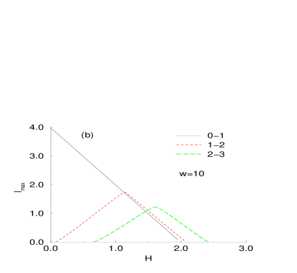
FIG. 1.: Plot of the maximum tunneling current as a function of applied magnetic field for a short junction with: (a) $w=1.0$ and (b) $w=10$.

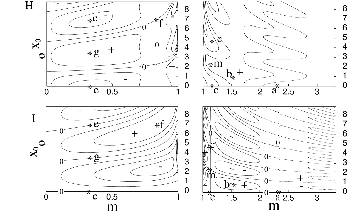
FIG. 2.: Constant $H$ (a) and $I$ (b) contours in the ($m$, $x_{0}$) plane. The curves with the symbol $O$ are for $H=0$ in (a) and $I=0$ in (b). The signs $"+"$ or $"-"$ give the sign of $I$ and $H$. The letter symbols signify the same points in the $I$ and $H$ contours.

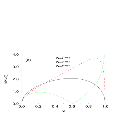
FIG. 3.: (a) Plot of $I(m)$ (using Eq. (13)) with $x_{0}=-K(m)$ or $K(m)$ and three values of $w$: (i) $w=2\pi/3$, (ii) $w=3\pi/2$ and (iii) $w=5\pi/2$. (b) Same as (a) with $w=10$ (dashed line). The right lobe in (b) is also shown in an expanded scale for $m$ (solid line). The small $m$ scale is shown at the top of the figure.

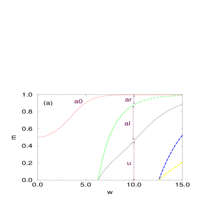
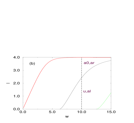
FIG. 4.: (a) A diagram of the different solutions in the space of parameter $w$ and $m$ with $x_{0}=\pm K(m)$ for the solutions in equations (13)-(15). (b) The same as (a) but presented in the space of $w$ and $I$ (instead of $m$).

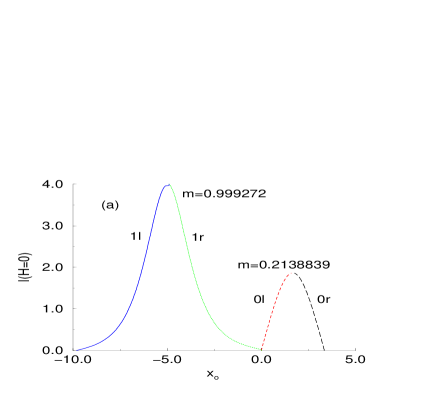
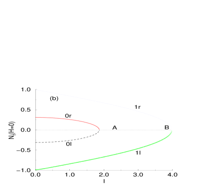
FIG. 5.: (a) Plot of $I(x_{o})$ for $H=0$, $w=10$ and fixed $m$ with (i) $m^{*}=0.999272$ (curves $1l$ and $1r$) from $w=2K(m^{*})$, (ii) $m^{*}=0.213839$ (curves $0l$ and $0r$) from $w=6K(m^{*})$. (b) Fluxon content $N_{f}$ as a function of the bias current $I$ for the different solutions with fixed $m$: (i) $m$=0.999272 with one half period of the elliptic function ($1r$ and $1l$). (ii) $m$=0.213839 with three half periods of the elliptic function ($0l$ and $0r$).

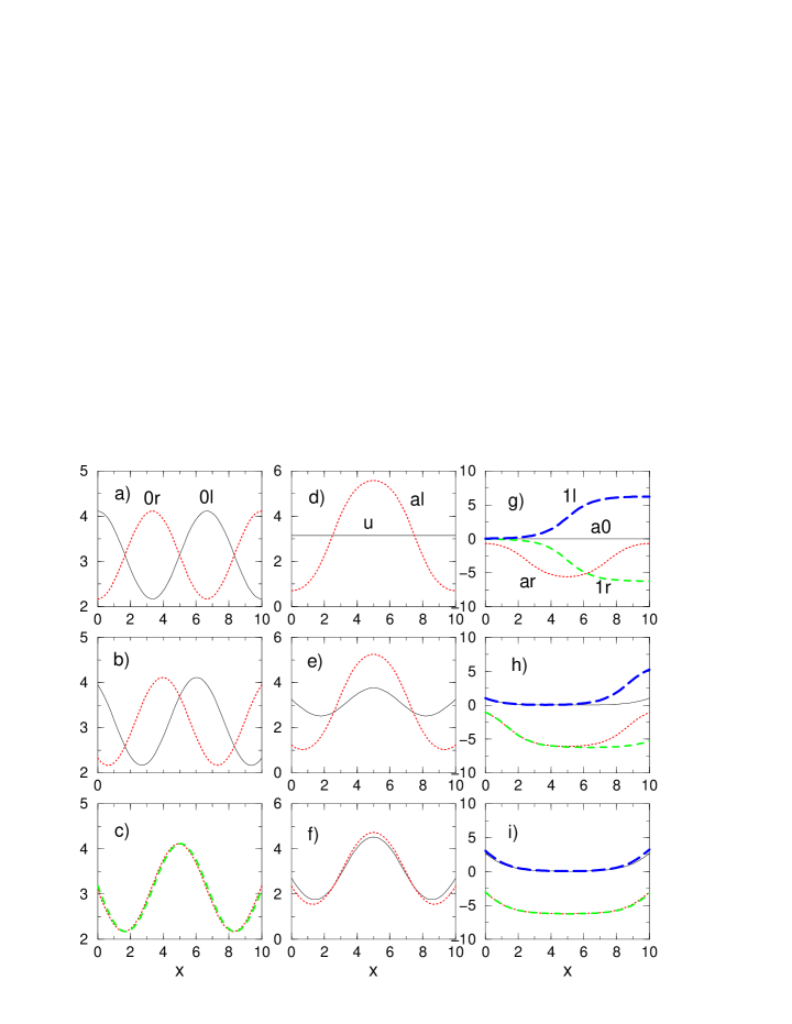
FIG. 6.: Plot of the phase distribution $\Phi(x)$ for all the solutions at $H=0$ and three values of the current (different for each line). ($a,~{}d,~{}g$) $I=0$, ($b,~{}e,~{}h$) $I=I_{max}/2$, ($c,~{}f,~{}i$) $I=I_{max}$ (where $I_{max}$ is different for each case). The three columns correspond to: ($a,~{}b,~{}c$) the two solutions $(0l,~{}0r)$ with $m^{*}=0.213839$. ($d,~{}e,~{}$f) the two solutions ($u$, $al$) from the left lobe of Fig. 3b and ($g,~{}h,~{}i$) the two solutions ($1r,~{}1l$) for $m^{*}=0.999272$ and the two solutions from the left lobe of Fig 5a (i.e. $a0,~{}ar$)

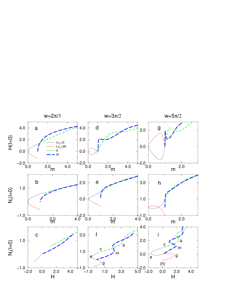
FIG. 7.: Plots of $H$ vs $m$ (top figures) and of the fluxon content $N_{f}$ for $I=0$ as a function of $m$ (middle figures) and $H$ (bottom figures), for a junction of length $w=\frac{2\pi}{3}$, $\frac{3\pi}{2}$, $\frac{5\pi}{2}$.

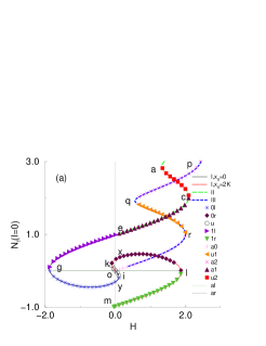
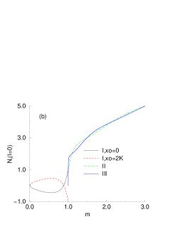
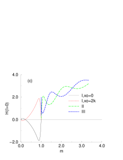
FIG. 8.: Plot of the fluxon content $N_{f}$ for $I=0$ and $w=10$ as a function of (a) $H$ and (b) $m$. In (c) we give $H(m)$.

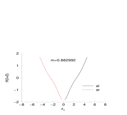
FIG. 9.: Magnetic field $H(x_{0})$ at $I=0$ for the constant $m=0.882992$ solution.

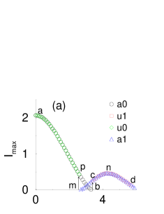
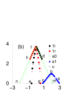
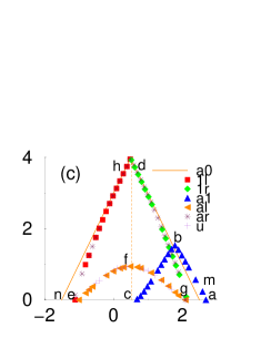
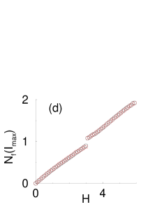
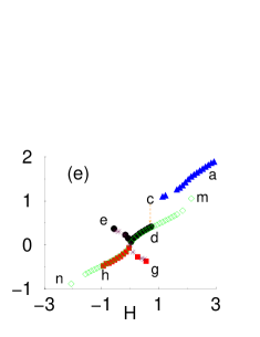
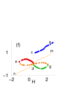
FIG. 10.: Maximum tunneling current as a function of $H$ for three different lengths (a) $w=\frac{2\pi}{3}$, (b) $w=\frac{3\pi}{2}$, (c) $w=\frac{5\pi}{2}$ and $N_{f}$ vs $H$ at the maximum current (d),(e),(f) correspondingly for the three lengths.

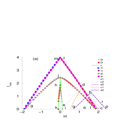
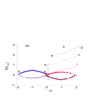
FIG. 11.: The same as Fig. 10 for $w=10$. (a) $I_{max}(H)$, (b) $N_{f}(H)$ at $I=I_{max}$.

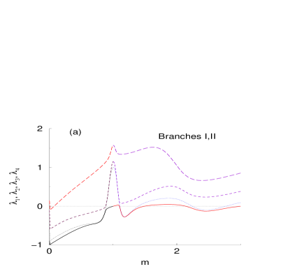
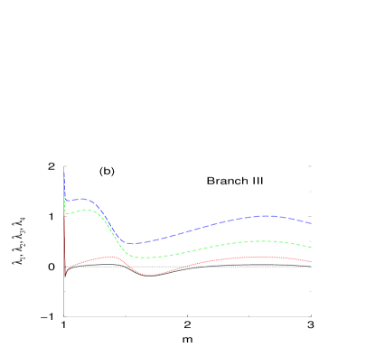
FIG. 12.: Plot of four lowest eigenvalues as a function of $m$ for (a) branches $I$ and $II$ and (b) branch $III$.

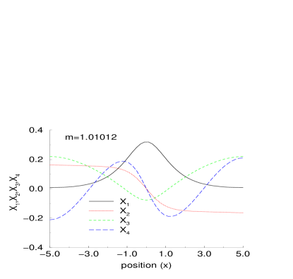
FIG. 13.: Plot of four lowest eigenmodes for $m=1.01012$ of branch $II$.

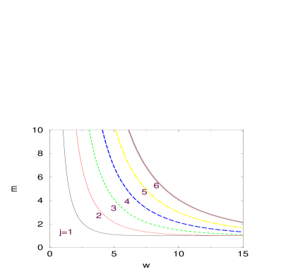
FIG. 14.: Plot of the neutral stability lines of integer $N_{f}$ in an $m$ vs $w$ diagram.

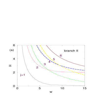
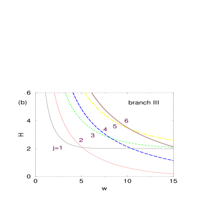
FIG. 15.: Same as Fig. 14 in an $H$ vs $w$ plot. (a) branch I and II and (b) branch III.

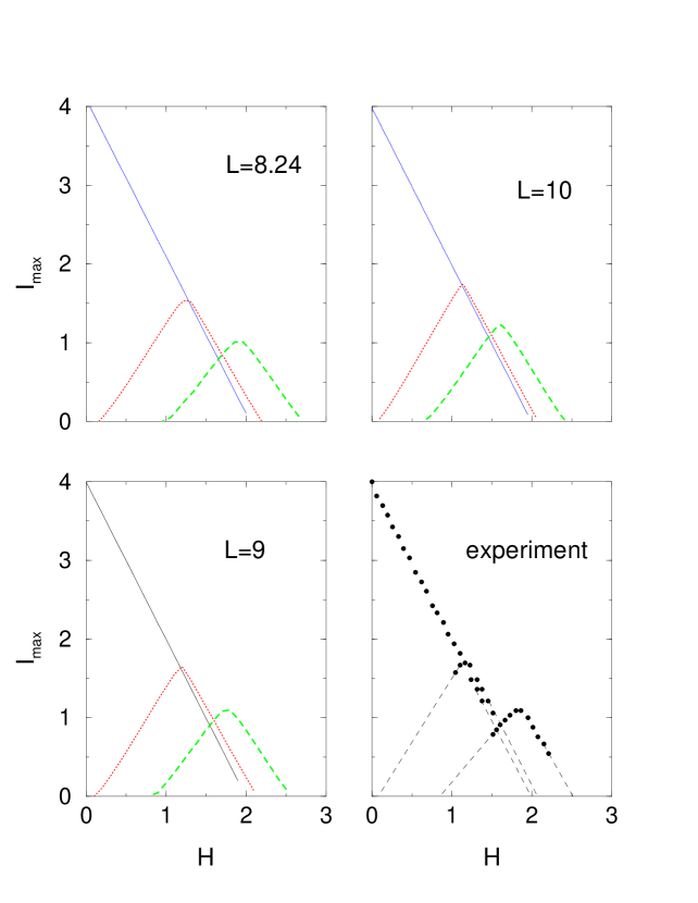
FIG. 16.: Numerical results for $I_{max}$ vs $H$ for $L=8.24$, $L=9$ and $L=10$ and the experimental data from [1]. In the experimental data the dots are the measured points and the dashed lines should only be considered as a guide for the eye.

FIG. 17.: Constant $H$ and $I$ contours in the ($m$, $x_{0}/K(m)$) plane.

REFERENCES

- [1] A. Barone and G. Paterno. Physics and Applications of the Josephson effect, John Wiley, New York, (1982).
- [2] A. Callegari and E. Reiss, J. Math. Phys. 14, 267 ( 1973).
- [3] R. Dickey, ”Stability theory for the damped Sine–Gordon equation”, SIAM J. Appl. Math., 30, 248–262 (1976).
- [4] R. Flesch and M.G. Forest and A. Sinha, Physica D 48, 169–231 (1991).
- [5] D. Brown and M. Forest and B. Miller and N. Petersson, SIAM J. Appl. Math., 54, 1048–1066 (1994).
- [6] J. G. Caputo, N. Flytzanis, and E. Vavalis, A semi–linear elliptic PDE model for static solution of josephson junctions, Int. J. Modern Physics C 6, 241 (1995).
- [7] R. Bank, PLTMG: A software package for solving elliptic partial differential equations. Users’ guide 8.0, SIAM, Philadelphia, (1998).
- [8] C.S. Owen and D.J. Scalapino, Vortex structure and critical currents in josephson junctions, Phys. Rev., 164, 538–544, (1967).
- [9] M. Abramowitz and I. A. Stegun, Handbook of Mathematical Functions, Dover, New York, (1965).
- [10] J. G. Caputo, N. Flytzanis and E. Vavalis, Int. J. Modern Physics, C 7, 191 (1996).
- [11] J.R. Rice and R.F. Boisvert, Solving Elliptic Problems Using ELLPACK, Springer-Verlag, New York, (1985).
- [12] J. G. Caputo, N. Flytzanis, Y. Gaididei and E. Vavalis, Phys. Rev. E 54, 2092 (1996).
- [13] R. Agoerst and R. Georg, Numerical continuation methods, Springer-Verlag, New York, (1985).
- [14] N. Alexeeva and T. Boyadjiev, Bulgarian Jour. of Physics, 24, 63-73 (1997).
- [15] L. Landau and I. Lifshitz, Classical Mechanics, Pergamon Press, (1987).
- [16] Yu. S. Kivshar, N. Gronbech-Jensen, and M. R. Samuelsen, Phys. Rev. B 45, 7789 (1992).