[

Cellular Dynamical Mean Field Approach to Strongly Correlated Systems

Abstract

We propose a cellular version of dynamical-mean field theory which gives a natural generalization of its original single-site construction and is formulated in different sets of variables. We show how non-orthogonality of the tight-binding basis sets enters the problem and prove that the resulting equations lead to manifestly causal self energies.

]

Dynamical mean field theory (DMFT) has been very successful in describing many aspects of strongly correlated electron systems [1], and presently much effort is put into implementing it for realistic calculations of materials properties of solids. By construction, this method describes correctly local correlations but misses altogether the effect of short-range order. This can be understood by noticing that in the limit of large lattice coordination ($z\rightarrow\infty$) [2] where the single-site DMFT is exact, the interactions which induce short-range correlations, such as magnetic superexchange, are scaled as $1\over z$ and in the absence of frozen correlations with $z$ neighbors they disappear from the problem. The effects of magnetic correlations on single-particle properties are captured by single site DMFT in magnetically ordered phases [3, 4]. However many applications require generalizations of the DMFT to capture short-range correlations, in the absence of broken symmetries. This is an active area of research and several methods have already been put forward [1, 5, 6, 7, 8] for this purpose.

The intuitive idea behind cluster methods is to treat certain local degrees of freedom (cluster degrees of freedom) exactly while replacing the remaining degrees of freedom by a bath of non interacting electrons which hybridize with the the cluster degrees of freedom so as to restore the translation invariance of the original problem. The simplest example of this idea is the Bethe Peierls cluster. The basic difficulty of a cluster technique is determining a suitable self consistency condition without generating unphysical solutions which violate causality. For a discussion of this longstanding problem in the context of disordered systems see [9]. Ingersent and Schiller[5] and independently Georges and Kotliar[1], introduced a truncation of the skeleton expansion in real space, which can be represented by solving coupled impurity models of different sizes. This method is not manifestly causal, but recent work [7], suggests that the problems with causality encountered in the earlier treatments are the result of inaccurate approximations in the solutions of the impurity models. Jarrell [6] and collaborators have suggested an alternative cluster scheme, the dynamic cluster approximation (DCA) which is a cluster scheme in momentum space, whereby the cluster considered, if regarded in real space has periodic boundary conditions. This body of work [6] and its extensions [8] established the computational feasibility and the existence of an a priori causal cluster schemes.

In this paper we pursue generalizations of the single site DMFT inspired by analogies with electronic structure methods. This cellular DMFT (CDMFT), remains close in spirit to the DMFT ideas described in the introduction, where the clusters have free (and not periodic) boundary conditions. We prove two central points:

I) The DMFT construction [1] can be carried out in a large class of basis sets. This observation frees us from the need to introduce sharp boundaries in real space. This approach is inspired by ideas from electronic structure, in which one achieves a cellular description by means of orbitals which can have a variable spatial extension.

II) This CDMFT construction is manifestly causal, i.e. the self energies that result from the solution of the cluster equations obey $\mbox{Im}\Sigma(k,\omega)\leq 0$, eliminating a priori one of the main difficulties encountered earlier in devising practical cluster schemes.

It is useful to to separate the three essential elements of a cluster scheme (see Fig. 1):

a) The definition of the cluster degrees of freedom, which are represented by impurity degrees of freedom in a bath described by a Weiss field matrix function $\widehat{G}_{0}$. The solution of the cluster embedded in a medium results in a cluster Green’s function matrix and a cluster self energy matrix.

b) The expression of the Weiss field in terms of the Green’s function or the self energy of the cluster, i.e. the self-consistency condition of the cluster scheme.

c) The connection between the cluster self energy and the self energy of the lattice problem. The impurity solver estimates the local correlations of the cluster, while the lattice self energy is projected out using additional information, i.e. the periodicity of the original lattice.

Our construction applies to very general models for which a lattice formulation naturally appears. It can be thought of as an extension of the band structure formalism that takes into account the electron electron interactions. The lattice Hamiltonian, $H[f_{i\sigma},f^{\dagger}_{i\sigma}]$, (one example could be the well known Hubbard Hamiltonian) is expressed in terms of creation and annihilation operators $f_{i\sigma}$ and $f^{\dagger}_{i\sigma}$ where $i$ runs over the sites of a d dimensional infinite lattice $i=(i_{1},\ldots,i_{d})$, the index $\sigma$ denotes an internal degree of freedom such as a spin index or a spin-orbital or band index if we consider an orbitally degenerate solid.

a) Selection of cluster variables: The first step in a mean field approach to a physical problem, is a selection of a finite set of relevant variables. This is done by splitting the original lattice into clusters of size $\prod_{j=1}^{d}$L_j arranged on a superlattice with translation vectors $R_{n}$. On this superlattice we choose wave functions $|R_{n}\alpha\rangle$ partially localized around $R_{n}$ with $\alpha=1,\ldots,N$ denoting an internal cluster index. The relation between the new wave functions, $|R_{n}\alpha\rangle$, and the old ones, $|i\sigma\rangle$, is encoded in a transformation matrix, $S_{R_{n}\alpha,i\sigma}$, such that $|R_{n}\alpha\rangle=\sum_{i\sigma}|i\sigma\rangle S^{-1}_{i\sigma,R_{n}\alpha}$. Due to the translation symmetry of the lattices we have $S_{R_{n}\alpha,i\sigma}=S_{\alpha\sigma}(r(i)-R_{n})$ where $r(i)$ is the position of site $i$. The creation and annihilation operators of the new basis are related to the operators of the old basis by $c_{R_{n}\alpha}=\sum_{i\sigma}S_{R_{n}\alpha,i\sigma}f_{i\sigma}$ and the operators that contain the ”local” information that we want to focus our attention on are $c_{\alpha}\equiv c_{(R_{n}=0)\alpha}$, i.e. the operators of the cluster at the origin. We will refer to these operators as the cluster operators. Note that we do not require that the wave function basis is orthogonal, and the nonorthogonality is summarized in an overlap matrix $O^{mn}_{\mu\nu}=O_{\mu\nu}(R_{m}-R_{n})\equiv\langle R_{m}\mu|R_{n}\nu\rangle$.

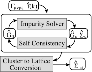
FIG. 1.: Schematic separation of the elements of a cluster dynamical mean field algorithm.

The next step is to express the Hamiltonian in terms of the complete set of operators $c_{R_{m}\mu}$. In terms of the new set of variables it has the form

$$H = -\sum_{R_{m}\mu R_{n}\nu}t_{\mu\nu}(R_{m}-R_{n})c_{R_{m}\mu}^{+}c_{R_{n}\nu}$$ (1)

$$+ \sum_{R_{1}\mu R_{2}\nu R_{3}\rho R_{4}\varsigma}U_{\mu\nu\rho\varsigma}(\{R_{i}\})c_{R_{1}\mu}^{+}c_{R_{2}\nu}^{+}c_{R_{4}\varsigma}c_{R_{3}\rho}.$$ (2)

We stress again that the generality of the method. Equation (2) has the form one would obtain by writing the full Hamiltonian of electrons in a solid in some tight binding non-orthogonal basis. The Hamiltonian is now split into three parts, $H=H_{c}+H_{cb}+H_{b}$ where $H_{c}$ involves only the cluster operators, $H_{b}$ contains $c_{R_{n}\mu}$ with $R_{n}\neq 0$ only and plays the role of a ”bath”, and finally $H_{cb}$ contains both $c_{R_{n}\mu}$ with $R\neq 0$ and the cluster operators $c_{\mu}$. Physically $H_{cb}$ couples the cluster with its environment. A similar separation can be carried out at the level of the action, in the coherent state functional integral formulation of this problem, where the partition function and the correlation functions are represented as averages over Grassman variables,

$$Z=\int\prod_{R_{n}\alpha}Dc^{+}_{R_{n}\alpha}Dc_{R_{n}\alpha}e^{-S}$$ (3)

where the action is given by

$$S = \int^{\beta}_{o}\!\!d\tau\left(\sum_{R_{m}\mu R_{n}\nu}\!c^{+}_{{R_{m}\mu}}O^{mn}_{\mu\nu}\partial_{\tau}c_{{R_{n}\nu}}-H[c^{+}_{{R_{m}\mu}},c_{{R_{n}\nu}}]\right)$$ (4)

$$\equiv S_{c}+S_{cb}+S_{b}.$$ (5)

The effective action for the cluster degrees of freedom is obtained conceptually by integrating out all the variables $c_{R_{n}\mu}$ with $R_{n}\neq 0$ in a path integral to obtain an effective action for the cluster variables $c_{\mu}$, i.e.

$${{1}\over{Z_{eff}}}e^{-S_{eff}[c^{+}_{\mu}c_{\mu}]}\equiv{{1}\over{Z}}\int\prod_{R_{m}\neq 0,\mu}Dc^{+}_{R_{m}\mu}Dc_{R_{m}\mu}e^{-S}.$$ (6)

Note that the exact knowledge of $S_{eff}$ allows us to calculate all the local correlation functions involving cluster operators. As described in [1], this cavity construction if carried out exactly would generate terms of arbitrary high order in the cluster variables. Our approximation neglects the renormalization of the quartic and higher order terms. Since the action $S_{cb}$ contains only boundary terms, the effects of these operators will decrease as the size of the cluster increases. Within these assumptions, the effective action is parameterized by $G_{0,\mu\nu}(\tau-\tau^{\prime})$, the Weiss function of the cluster and has the form

$$S_{eff} = -\int^{\beta}_{0}\!\!\!\!d\tau d\tau^{\prime}\sum_{\mu\nu}c^{+}_{\mu}(\tau)G_{0,\mu\nu}^{-1}(\tau-\tau^{\prime}){c_{\nu}}(\tau^{\prime})$$ (8)

$$+\int^{\beta}_{0}\!\!\!\!d\tau_{1}d\tau_{2}d\tau_{3}d\tau_{4}\Gamma_{\mu\nu\rho\varsigma}c^{+}_{\mu}(\tau_{1})c^{+}_{\nu}(\tau_{2})c_{\varsigma}(\tau_{4})c_{\rho}(\tau_{3})$$

where $\Gamma_{\mu\nu\rho\varsigma}=U_{\mu\nu\rho\varsigma}(\{0\})$. Using the effective action (8) one can calculate the Green’s functions of the cluster $G_{c,\mu\nu}(\tau-\tau^{\prime})[\widehat{G}_{0}]\equiv-\langle T_{\tau}c_{\mu}(\tau)c^{+}_{\nu}(\tau^{\prime})\rangle[\widehat{G}_{0}]$ and the cluster self energies

$$\widehat{\Sigma}_{c}\equiv\widehat{G}_{0}^{-1}-\widehat{G}_{c}^{-1}.$$ (9)

b) Self-consistency condition: The cluster algorithm is fully defined once a self-consistency condition which indicates how $\widehat{G}_{0}$ should be obtained from $\widehat{\Sigma}_{c}$ and $\widehat{G}_{c}$ is defined. In the approach that we propose here the self consistent equations become matrix equations expressing the Weiss field in terms of the cluster self energy matrix $\widehat{\Sigma}_{c}$.

$$\widehat{G}_{0}^{-1}=\left(\sum_{k}\frac{1}{(i\omega+\mu)\widehat{O}(k)-\widehat{t}(k)-\widehat{\Sigma}_{c}}\right)^{-1}+\widehat{\Sigma}_{c}$$ (10)

where $\widehat{O}(k)$ is the Fourier transform of the overlap matrix, $\widehat{t}(\mathbf{k})$, is the Fourier transform of the kinetic energy term of the Hamiltonian in Eq. (2) and k is now a vector in the Brillouin zone (reduced by the size of the cluster, L_j, in each direction). Equations (8) and (10), can be derived by scaling the hopping between the supercells as the square root of the coordination raised to power of the Manhattan distance between the supercells and generalizing the cavity construction of the DMFT [1] from scalar to matrix self energies. If the cluster is defined in real space and the self energy matrices could be taken to be cyclic in the cluster indices so that the matrix equations could be diagonalized in a cluster momentum basis, Eq. (10) would reduce to the DCA equation[6]. However, in the DMFT construction, the clusters have free and not periodic boundary conditions, and we treat a more complicated problem requiring additional matrix inversions.

c) Connection to the self energy of the lattice: The self-consistent solution, $\widehat{G}_{c}$ and $\widehat{\Sigma}_{c}$, of the cluster problem can be related to the correlation functions of the original lattice problem through the transformation matrix $S_{R_{m}\alpha,i\sigma}$ by the equation

$$\Sigma_{lat,\sigma\sigma^{\prime}}(k,\omega)=\sum_{\mu\nu}\tilde{S}^{\dagger}_{\sigma,\mu}(k)\Sigma_{c,\mu\nu}(\omega)\tilde{S}_{\nu,\sigma^{\prime}}(k)$$ (11)

where $\tilde{S}$ is the Fourier transform of the matrix S with respect to the original lattice indices i. Notice that $\Sigma_{lat,\sigma\sigma^{\prime}}$ is diagonal in momentum and will also be diagonal in the variable $\sigma$ if this variable is conserved.

d) Connection to impurity models: As in single site DMFT it is very convenient to view the cluster action as arising from a Hamiltonian,

$$H_{imp} = \sum_{\rho\varsigma}\widehat{E}_{\rho\varsigma}c^{+}_{\rho}c_{\varsigma}+\sum_{\mu\nu\rho\varsigma}\Gamma_{\mu\nu\rho\varsigma}c^{+}_{\mu}c^{+}_{\nu}c_{\rho}c_{\varsigma}$$ (12)

$$+ \sum_{k\lambda}\epsilon_{k\lambda}a^{+}_{k\lambda}a_{k\lambda}+\sum_{k\lambda,\mu}\left(V_{k\lambda,\mu}a^{+}_{k\lambda}c_{\mu}+h.c.\right).$$ (13)

Here $\epsilon_{k\lambda}$ is the dispersion of the auxiliary band and $V_{k\lambda,\mu}$ are the hybridization matrix elements describing the effect of the medium on the impurity. When the band degrees of freedom are integrated out the effect of the medium is parameterized by a hybridization function,

$$\Delta_{\mu\nu}(i\omega_{n})[\epsilon_{k\lambda},V_{k\lambda}]=\sum_{k\lambda}\frac{V^{*}_{k\lambda,\mu}V_{k\lambda,\nu}}{i\omega_{n}-\epsilon_{k\lambda}}.$$ (14)

The hybridization function is related to the Weiss field function by expanding Eq. 10 in high frequencies:

$$\widehat{G}_{0}^{-1}(i\omega_{n})=i\omega_{n}\bar{O}-\widehat{E}-\widehat{\Delta}(i\omega_{n})$$ (15)

with $\bar{O}=\left[\sum_{k}\widehat{O}_{k}^{-1}\right]^{-1}$ indicating that the impurity model has been written in a non-orthogonal local basis with an overlap matrix $\bar{O}$.

Let us now consider some examples of this approach.

a) Single-site DMFT: The simplest example is the single-site dynamical mean field theory which is exact in the limit of infinite dimensions. In this case the cluster is just a single site denoted by 0, and the cluster operators are the creation and annihilation operators of that site $c^{+}_{o\sigma}$, $c_{o\sigma}$. The cluster Hamiltonian is diagonal in the spin variables and reduces to the effective action of the Anderson impurity model. The second step is a scalar equation $\widehat{G}_{0}^{-1}=\widehat{G}_{c}^{-1}[G_{0}]+\widehat{\Sigma}_{c}[G_{0}]$. Finally the third step identifies the self energy of the cluster with the lattice self energy.

b) Free cluster: The next example is a free cluster scheme for the one band Hubbard model. The method divides the lattice into supercells, and views each supercell as a complex ”site” to which one can apply ordinary DMFT. Here $R_{n}$ is the supercell position and $\alpha$ labels the different sites within the unit cell, and the spin. Introducing a spin label $\sigma$ and a supercell notation where an atom is denoted by the supercell, $R_{n}$, and the position inside the supercell, $l$; $\alpha=(\sigma^{\prime},l)$ and $S_{R_{n}\alpha,i\sigma}=\delta_{\sigma,\sigma^{\prime}}\delta_{R_{n}+l,r_{i}}$ is diagonal in spin and position. In this case the overlap matrix is the identity. This real space cluster method has been investigated using quantum Monte Carlo methods (QMC) by Katsnelson and Lichtenstein [10].

c) Multiorbital DMFT in a non-orthogonal basis: Another important special case of our general construction is the implementation of single-site DMFT in a non-orthogonal basis. In this case the supercell is a single site, but the wave functions defining the cluster operators are chosen so that they are very localized in real space.

In fact, an implementation of this method, in conjunction with a generalization of the interpolative perturbation theory, as an impurity solver, has resulted in new advances in the theory of Plutonium [11] Here the flexibility in the choice of basis is crucial for the success of the DMFT program. DMFT neglects from the start interactions which are not onsite. A high degree of localization requires a non-orthogonal basis and the formalism introduced in this letter.

d) Other bases: Finally we point out that the most attractive feature of this method is that it would allow its formulation in terms of wave functions which are partially localized in real and momentum space such as wavelet functions. This flexibility is most appealing for treating problems such as the Mott transition where both the particle-like and the wave-like aspect of the electron need to be taken into account requiring a simultaneous consideration of real and momentum space.

We now prove that the CDMFT approach gives manifestly causal Green’s functions. For this we assume, that we start the DMFT iteration with a guess for the bath function $\widehat{\Delta}$ which is causal. The self energy which is generated in the process of solving the ”impurity model” is also causal. Furthermore, any sensible approximation techniques to compute the self energy of the cluster respects causality, so our proof is valid not just for exact solutions of the CDMFT scheme but also for approximate solutions as long as the impurity solvers used in the solution of the cluster impurity problem preserve causality. The next step is to show that if a causal self energy is introduced in the self-consistency condition, (10), the resulting bath function $\widehat{\Delta}$ is causal. Since both $\widehat{\Sigma}_{c}$ and $\widehat{\Delta}$ are matrices, the causality condition needs to be formulated precisely. For a Fermionic matrix function, $A(\omega)$, to be causal means that it is analytic in the upper half of the complex frequency plane and thus has a spectral representation with spectral density $\frac{-1}{2\pi i}\{A(\omega)-A^{\dagger}(\omega)\}$, and the spectral density matrix is positive definite. It is easy to see that the DMFT equations lead to the correct analytic properties and the following proof establishes the positivity of the bath spectral density. Writing $\Sigma_{R}=\epsilon-i\gamma$ with $\epsilon$, $\gamma$ hermitian and $\gamma$ positive definite, we get:

$$(\widehat{\Delta}_{R}^{\dagger}-\widehat{\Delta}_{R}) = -2i\gamma$$ (17)

$$+\sqrt{\gamma}\left(\left\{\sum_{k}\frac{1}{i+d_{k}}\right\}^{-1}-\left\{\sum_{k}\frac{1}{-i+d_{k}}\right\}^{-1}\right)\sqrt{\gamma}.$$

Positivity is reduced to proving that the following matrix is negative [12], i.e.

$$2-\left\{\sum_{k}\frac{1}{1-id_{k}}\right\}^{-1}-\left\{\sum_{k}\frac{1}{1+id_{k}}\right\}^{-1}\leq 0.$$ (18)

Here $\omega\widehat{O}(k)-\widehat{t}(k)-\epsilon\equiv\sqrt{\gamma}d_{k}\sqrt{\gamma}$. Performing a change of variables $d_{k}=i{{{{e^{i\theta_{k}}}}+{{e^{-i\theta_{k}}}}}\over{{{e^{i\theta_{k}}}}-{{e^{-i\theta_{k}}}}}}$ with ${\theta_{k}}$ a hermitian matrix, Eq. (18) reduces to proving that

$$1\leq\min_{x}{{\langle x|(1-z)^{-1}+(1-z^{\dagger})^{-1}|x\rangle}\over{\langle x|x\rangle}}$$ (19)

where $z\equiv\langle\!\langle e^{-2i{\theta_{k}}}\rangle\!\rangle$ , with $\langle\!\langle\rangle\!\rangle$ denoting an average over the Brillouin zone. By performing the substitution $|x\rangle=(1-z)|y\rangle$ Eq. (19) reduces to

$$1\leq\min_{||y||=1}\frac{2+\langle y|z+z^{\dagger}|y\rangle}{1+\langle y|z^{\dagger}z|y\rangle+\langle y|z+z^{\dagger}|y\rangle}$$ (20)

which clearly holds due to the fact that $z$ is an average of unitary matrices, and has the property $||z^{\dagger}z||\leq 1$. From Eq. (20) and Eq. (11) it follows that the imaginary part of the retarded self energy is always less or equal to zero, completing the proof of causality. This proof generalizes Ref. [6] from scalar to matrix CPA equations.

In conclusion DMFT has produced a wealth of information in problems where the physics is local and cluster methods promise to be equally fruitful in more complex problems where correlations between more sites and orbitals need to be taken into account. All the techniques which have been used for the solution of the single site DMFT are applicable to this cluster extension. The most powerful methods of solution have been renormalization group related techniques such as the projective self-consistent method [13] or the numerical Wilson renormalization group techniques [14]. These methods carry out a division of the impurity and the bath into a low-energy and a high-energy part, and perform an elimination of the high-energy degrees of freedom in both. Extensions of these methods to an abstract cluster is a first step in constructing non-perturbative renormalization group method for correlated fermion systems and deserves further investigations.

REFERENCES

- [1] A. Georges, G. Kotliar, W. Krauth and M. J. Rozenberg, Rev. Mod. Phys. 68 13 (1996).
- [2] W. Metzner and D. Vollhardt, Phys. Rev. Lett. 62, 324 (1989).
- [3] R. Chitra and G. Kotliar, Phys. Rev. Lett. 83, 2386 (1999).
- [4] Marcus Fleck, Alexander I. Lichtenstein, Eva Pavarini and Andrzej M. Oles, Phys. Rev. Lett. 84, 4962 (2000).
- [5] S. Schiller and K. Ingersent, Phys. Rev. Lett. 75, 113 (1995).
- [6] C. Huscroft et al., cond-mat/9910226; M. H. Hettler, M. Mukherjee, M. Jarrell and H. R. Krishnamurthy, cond-mat/9903273; T. Maier, M. Jarrell, T. Pruschke, J. Keller, Eur. Phys. J. B 13, 613 (2000); M. H. Hettler et al., Phys, Rev. B 58, R7475 (1998).
- [7] Gergely Zaránd, Daniel L. Cox, and Avraham Schiller, cond-mat/0002073.
- [8] A. Lichtenstein and M. Katsnelson cond-mat/9911320, Phys. Rev. B (in press).
- [9] R. J. Elliot, J. A. Krumhansl and P. L. Leath, Rev. Mod. Phys. 46, 465 (1974).
- [10] A. Lichtenstein (private communication).
- [11] S. Y. Savrasov et al. (in preparation).
- [12] The matrix inequality is defined by the condition for all vectors x.
- [13] G. Moeller, Q. Si, G. Kotliar, M. J. Rozenberg and D. S. Fisher, Phys. Rev. Lett. 74 2082 (1995).
- [14] R. Bulla, Phys. Rev. Lett. 83, 136 (1999).