Weak-coupling functional renormalization-group analysis of the Hubbard model on the anisotropic triangular lattice

Abstract

Motivated by experiments on the layered compounds $\kappa$-(BEDT-TTF)₂X, Cs₂CuCl₄, and very recently Na_xCoO${}_{2}\cdot y$H₂O, we present a weak-coupling functional renormalization-group analysis of the Hubbard model on the anisotropic triangular lattice. As the model interpolates between the nearest-neighbor square lattice and decoupled chains via the isotropic triangular lattice, it permits the study of competition between antiferromagnetic and BCS Cooper instabilities. We begin by reproducing known results for decoupled chains, and for the square lattice with only nearest-neighbor hopping amplitude $t_{1}$. We examine both repulsive and attractive Hubbard interactions. The role of formally irrelevant contributions to the one-loop renormalization-group flows is also studied, and these subleading contributions are shown to be important in some instances. We then observe that crossover to a BCS-dominated regime can occur even at half-filling when antiferromagnetism is frustrated through the introduction of a next-nearest-neighbor hopping amplitude $t_{2}$ along one of the two diagonal directions. Stripes are not expected to occur and time-reversal breaking $d_{x^{2}-y^{2}}\pm id_{xy}$ superconducting order does not arise spontaneously; instead pure $d_{x^{2}-y^{2}}$ order is favored. At the isotropic triangular point ($t_{1}=t_{2}$) we find the possibility of re-entrant antiferromagnetic long-range order.

I Introduction

The behavior of strongly correlated electrons moving in reduced spatial dimensions continues to yield surprising new physics. For example, intriguing experimentsWilliams ; Ishiguro ; McKenzie1 on the $\kappa$-(BEDT-TTF)₂X family of layered organic molecular crystals evoke similar findings in the field of high-temperature cuprate superconductivity. Like the high-T_c cuprates, the layered organic materials exhibit a wide variety of electronic properties. In particular, the phase diagram is rather similar to that of the cupratesMcKenzie2 and there is some evidence for unconventional pairing with nodes in the gap from NMR relaxation ratenmr1 ; nmr2 ; nmr3 , specific heatspecificheat , penetration depthpdepth1 ; pdepth2 ; pdepth3 ; pdepth4 ; pdepth5 , STM spectroscopystm , mm-wave transmissionmm1 (see however Refs. mm2, ; mm3, ) and thermal conductivitythermal1 ; thermal2 measurements. Other experiments, however, suggest $s$-wave pairingswave1 ; swave2 ; swave3 ; swave4 ; swave5 ; swave6 . Competition between antiferromagnetic and superconducting instabilities, seen in the cuprates, also seems to occur in the $\kappa$-(BEDT-TTF)₂X compoundsLefebvre . In contrast to the square CuO₂ lattice of the high-temperature superconductors, the organic molecules pair up into dimers, and these dimers form a triangular lattice.

Two other quasi two-dimensional materials with triangular lattices have been the subject of recent attention: The antiferromagnetic insulator Cs₂CuCl₄ compoundRadu and the cobalt-based superconductor Na_xCoO${}_{2}\cdot y$H₂O that may be an analog of the cuprate high-temperature superconductorsTakada . Neutron scattering experiments suggest the existence of deconfined spinon (spin-$1/2$) excitations in the Cs₂CuCl₄ once antiferromagnetic order has been eliminated by heating the sample to the relatively low temperature of approximately 0.6K, or upon application of a field parallel to the planeRadu . Geometric frustration of the spin-spin interactions is likely responsible for the observed spin-liquid behavior. As the cobalt atoms in the Na_xCoO${}_{2}\cdot y$H₂O material also form a triangular latticeBalsys , and as they have further been argued to carry spin-$1/2$ momentsTakada , we tentatively group this system into the same category as $\kappa$-(BEDT-TTF)₂X and Cs₂CuCl₄.

Clearly theoretical investigations of strongly correlated electrons on triangular lattices are of great interest. Initial studies of strongly correlated systems often start with a minimal Hubbard model, leaving extensions such as the inclusion of long-range Coulomb interactions for later more detailed work. In fact McKenzie has proposedMcKenzie2 that a Hubbard model on the anisotropic triangular lattice serves as a minimal model of the conducting layers of $\kappa$-(BEDT-TTF)₂X. It represents a simplification of a model introduced earlier by Kino and FukuyamaKino1 . Two distinct hopping matrix elements are introduced and the Hamiltonian is defined by:

$$H=-t_{1}\sum_{<{\bf ij}>}(c_{\bf i}^{\dagger\sigma}c_{{\bf j}\sigma}+H.c.)-t_{2}\sum_{<<{\bf ij}>>}(c_{\bf i}^{\dagger\sigma}c_{{\bf j}\sigma}+H.c.)+~{}U\sum_{\bf i}n_{{\bf i}\uparrow}n_{{\bf i}\downarrow}-\mu\sum_{\bf i}n_{\bf i},$$ (1)

where $<{\bf ij}>$ denotes nearest-neighbor pairs of sites on the square lattice and $<<{\bf ij}>>$ denotes next-nearest-neighbor pairs along one of the two diagonal directions of the square lattice as shown in Fig. 1. Quantum chemistry calculations suggest that, unlike the cuprate materials, in the case of the organic $\kappa$-(BEDT-TTF)₂X compounds the Hubbard interaction $U\approx t$. Thus a weak-coupling renormalization-group (RG) approach such as we adopt here may be expected to be reasonably accurate for the organic materials.

Figure 1: Anisotropic triangular lattice with two hopping amplitudes $t_{1}$ and $t_{2}$. The limit $t_{2}=0.0$ corresponds to the usual nearest-neighbor square lattice and $t_{1}=0.0$ corresponds to decoupled chains.

The model is also interesting in its own right as it interpolates between the square lattice and decoupled chains. At half-filling, the non-interacting Fermi surface is perfectly nested in these two extreme limits. As nesting is imperfect in between the limiting cases, several phase transitions can be expected. The square lattice, which has been the subject of many studies, corresponds to the special case of zero next-nearest-neighbor hopping, $t_{2}=0$. When the repulsive interaction is turned on, nesting induces a spin density wave instability. In the opposite limit, $t_{1}=0$, the chains are completely decoupled. These isolated chains of course have no spin order and are described by the exact Bethe ansatz solution of Lieb and WuLieb . We pay particular attention to the intermediate region of $t_{1}\neq 0$ and $t_{2}\neq 0$ and study it via a weak-coupling renormalization-group analysis. The special isotropic triangular lattice point corresponds to $t_{1}=t_{2}$. Values for the hopping matrix elements obtained from experiments and from quantum chemistry calculations for the conducting layer of $\kappa$-(BEDT-TTF)₂X suggest $t_{1}>t_{2}$, that is, somewhere intermediate between the square and the isotropic triangular limits. The lattice anisotropy can be altered by uniaxial stress applied along the principal axes of the quasi-two-dimensional organic compoundChoi . Fermi surfaces of non-interacting electrons for different ratios of the hopping matrix elements are shown in Fig. 2.

Figure 2: Fermi surface of non-interacting electrons for different ratios of the two hopping amplitudes. The number at the top of each graph is the anisotropy ratio $t_{2}/(t_{1}+t_{2})$ which ranges from $0$ (square lattice) to $1$ (decoupled chains). The chemical potential $\mu$ is varied to ensure that the system remains half-filled.

In the next section we briefly introduce the RG method we employ, a method first implemented by Zanchi and SchulzZanchi for the case of the square lattice. We then present results of our calculations at different values of the anisotropy: decoupled chains (studied as a test case to check the reliability of the calculation), square lattice, and finally the anisotropic region intermediate between the square lattice and the isotropic triangular lattice. We discuss the ordering tendencies and work out the implied phase diagram as a function of anisotropy parameter $t_{2}/(t_{1}+t_{2})$ which ranges from $0$ (square lattice) to $1$ (decoupled chains). We also make comparison to results obtained via other methods in the strong-coupling limit of large on-site repulsion.

II Renormalization-group calculation

We follow the weak-coupling renormalization-group analysis implemented by Zanchi and SchulzZanchi for interacting fermions on a two-dimensional lattice. Like some previous workHKM , the approach generalizes Shankar’s renormalization group theoryShankar to Fermi surfaces of arbitrary shape. More significantly, in principle the only approximation that is made in the approach of Zanchi and Schulz is an expansion in powers of the interaction strength, the on-site Coulomb interaction $U$. Subleading terms generated during the RG transformations, which are dropped as irrelevant in the simplest versions of the RG, are instead kept in this formulation. Specifically, the formally irrelevant, non-logarithmic, terms that appear in the six-point function during the process of mode elimination do in fact contribute to the RG flows. Thus while the simplest weak-coupling RG analyses makes a double expansion in both the interaction strength and in the relevance of the terms retained in the renormalization flows, in the approach of Zanchi and Schulz there is only a single expansion in the interaction strength. (In practice some additional approximations are made for computational convenience, as detailed below. These simplifications are not expected to alter the results significantly.) As we show below, in some cases this more accurate treatment leads to substantial differences in the RG flows.

Elimination of high energy modes is carried out iteratively, in infinitesimal steps, and as a result the energy cutoff $\Lambda$ around the Fermi surface shrinks, see Fig. 3. The initial energy cutoff is taken to be the full band width $\Lambda_{0}$, and it is reduced via continuous mode elimination to $\Lambda=\Lambda_{0}~{}e^{-\ell}$ where $\ell>0$.

Figure 3: Mode elimination is carried out in infinitesimal steps. The figure shows the low energy modes (denoted $L$) which are inside a shell of thickness $\Lambda$ around the Fermi surface, and the high energy modes ($H$), which have already been integrated out and which are now outside the shell. At each step the on-shell modes precisely at scaling parameter $\ell$ (dashed lines) are integrated out.

For each infinitesimal step $\ell\rightarrow\ell+d\ell$, the fermion degrees of freedom are broken down into high and low energy modes as

$$\Psi_{\sigma}(K)=\Theta(\Lambda-|\epsilon_{\bf k}|)~{}\Psi_{\sigma,L}(K)~{}+~{}\Theta(|\epsilon_{\bf k}|-\Lambda)~{}\Psi_{\sigma,H}(K)~{},$$ (2)

where $K\equiv(\omega,{\bf k})$ is the usual 2+1-dimensional frequency-momentum vector. The effective action, after dropping a constant contribution $\Omega_{H}$ to the free energy, has the form

$$S_{\Lambda(\ell+d\ell)}=S_{\Lambda(\ell)}+\delta S(\ell).$$ (3)

At non-zero $\ell>0$ the effective action contains contributions at all orders in the initial interaction strength. But because mode elimination is done in infinitesimal steps, only terms linear in $d\ell$ contribute to $\delta S(\ell)$. These terms correspond to diagrams with one internal line (either a loop or a tree diagram). RG flow equations for vertices with any number of legs, $\Gamma_{2n}(\ell)$, can then be found. These are functional equations since the $\Gamma$’s are functions of momenta and frequencies.

To make progress we must make an approximation. We carry out the weak-coupling expansion by truncating the RG equations at the one-loop level. Renormalization of the effective interaction $U_{\ell}({\bf k_{1}},{\bf k_{2}},{\bf k_{3}},{\bf k_{4}})$, corresponding to the four-point function ($\Gamma_{4}$), then occurs at order $U^{2}$. Contributions from the six-point functions $\Gamma_{6}$ must also be included at this order. Higher n-point functions may be neglected as these only contribute at higher-order in the interaction strength $U$. It is important to notice that the RG flow equations generated this way are non-local in scaling parameter $\ell$. The RG equations for couplings $U_{\ell}({\bf k_{1}},{\bf k_{2}},{\bf k_{3}},{\bf k_{4}})$ at step $\ell$ involve the values of couplings at previous steps $\ell_{pp}$ and $\ell_{ph}$ [the subscript denotes particle-particle (pp) and particle-hole (ph) channels]:

$$\ell_{pp}=-\ln\left(\frac{\epsilon_{{\bf k}-{\bf q_{pp}}}}{\Lambda_{0}}\right)$$ (4)

$$\ell_{ph}=-\ln\left(\frac{\epsilon_{{\bf k}+{\bf q_{ph}}}}{\Lambda_{0}}\right)$$ (5)

with ${\bf q_{pp}}={\bf k_{1}}+{\bf k_{2}}$ and ${\bf q_{ph}}={\bf k_{1}}-{\bf k_{4}}$. At step $\ell$ contributions from six-point functions are obtained by contracting two of the legs at on-shell momentum ${\bf k}$. Of course the six-point functions were generated from four-point functions during previous steps. Momentum ${\bf k_{4}}$ is determined uniquely by momentum conservation to be ${\bf k_{4}}={\bf k_{1}}+{\bf k_{2}}-{\bf k_{3}}$, so we drop it in the following.

For an initial, bare, four-fermion interaction $U_{0}$ which is independent of spin, following Zanchi and Schulz it is possibleZanchi to write all the renormalized two-particle interactions in terms of only one function $U_{\ell}({\bf k_{1}},{\bf k_{2}},{\bf k_{3}})$. Couplings in the charge and spin sectors can then be obtained from this function through the relations:

$$U_{c}=\frac{1}{4}(2-\hat{X})U,\hskip 72.26999ptU_{\sigma}=-\frac{\hat{X}}{4}U.$$ (6)

where $\hat{X}$ is a permutation operator defined by its action: $\hat{X}U({\bf k_{1}},{\bf k_{2}},{\bf k_{3}})\equiv U({\bf k_{2}},{\bf k_{1}},{\bf k_{3}})$. The charge density (CDW) and spin density (AF) couplings are then given by:

$$V_{\ell}^{CDW}(\theta_{1},\theta_{2}) = 4U_{c\ell}({\bf k_{1}},{\bf k_{2}},{\bf\tilde{k}_{1})}$$

$$V_{\ell}^{AF}(\theta_{1},\theta_{2}) = 4U_{\sigma\ell}({\bf k_{1}},{\bf k_{2}},{\bf\tilde{k}_{1})}\ .$$ (7)

Here ${\bf\tilde{k}}_{j}$ is related to ${\bf k}_{j}$ by ${\bf k}_{j}-{\bf\tilde{k}}_{j}={\bf Q}$ where ${\bf Q}$ is a nesting vector [${\bf Q}=(\pm\pi,\pm\pi)$ for the fully nested square lattice]. Also $\theta_{j}$ is the angle that wavevector ${\bf k}_{j}$ makes with the x-axis. The forward scattering amplitude is given by

$$F_{\ell}(\theta_{1},\theta_{2})=U_{\ell}({\bf k_{1}},{\bf k_{2}},{\bf k_{1}})$$ (8)

and only involves two momenta (${\bf k_{1}}$ and ${\bf k_{2}}$) because the momentum transfer during scattering is very small. Likewise the BCS interaction

$$V_{\ell}^{BCS}(\theta_{1},\theta_{2})=U_{\ell}({\bf k_{1}},-{\bf k_{1}},{\bf k_{2}})$$ (9)

also is described by just two momenta as it represents the scattering of a Cooper pair of electrons of opposing momenta ${\bf k_{1}}$ and ${\bf-k_{1}}$ into a pair of electrons of opposing momenta ${\bf k_{2}}$ and ${\bf-k_{2}}$.

Figure 4: Discretization of the Fermi surface into $M=16$ patches. Each patch corresponds to an angular section of $2\pi/M$. The special case of the perfectly-nested Fermi surface corresponding to the nearest-neighbor tight-binding model on a square lattice and at half-filling is shown.

In order to integrate the flow equations forward in the scaling parameter $\ell$ we first discretize the Fermi surface, dividing it up into patches as depicted in Fig. 4. Replacing the continuous surface with discrete patches should be adequate for the imperfectly nested Fermi surfaces we focus on hereDoucot . After discretization of the Fermi surface, the angles $\theta_{j}=2\pi j/M$ where $j=0,\ldots,M-1$. Interactions $U_{\ell}(i_{1},i_{2},i_{3})$ are thus labeled by three discrete patch indices. A further approximation is implied by this procedure, as the dependence of the effective interaction on the radial component of momentum is neglected and the shape of the Fermi surface is not renormalized. The justification is the following: though the shape of the Fermi surface change at the one-loop level, the feedback of this change on the one-loop RG flows for the couplings $U_{\ell}(i_{1},i_{2},i_{3})$ constitutes a higher-order effect. The dependence of $U$ on the radial components of the three momenta is irrelevantZanchi2 ; Shankar . This is similar to the one-dimensional case, where the marginal interactions are labeled according to the indices $i=L,R$ (left or right moving) of the electrons that are interacting. There is strong dependence on the direction of ${\bf k}$, but the dependence on the absolute value $|{\bf k}|$ of the momentum is irrelevant. Therefore the interactions may be parameterized simply by their projection onto the two Fermi points. In two dimensions the interactions are likewise parameterized by the patch indices.

In this work we only study flows at zero temperature. The integral over Matsubara frequencies, which arises in the one-loop diagram, can be performed analytically as the dependence of the couplings on the frequency $\omega$ is irrelevantZanchi2 . We set the initial bare coupling to be $|U_{0}|=1$ and, unless otherwise stated, also set $t_{1}+t_{2}=1$. The full band width is $\Lambda_{0}=8t_{1}+4t_{2}$. We usually divide the Fermi surface into $M=16$ patches. For the special case of the isotropic triangular lattice we instead use a finer mesh of patches, $M=24$, to permit an examination of higher-wave channels. Our algorithm makes no assumptions about the symmetries of the Fermi surface; this means that we must follow the flow of all $M^{3}$ couplings $U(i_{1},i_{2},i_{3})$. We do impose the requirement that the three indices are such that all four particles lie on the Fermi surface. The RG flow for these couplings are then described by coupled non-local integral-differential equations. These equations are numerically integrated forward in the scaling parameter $\ell$. The increment in the scaling parameter is set to be $d\ell=0.1$ for the results shown here. Calculations using smaller values of $d\ell$ yield nearly the same results.

An equivalent version of RG method for two-dimensional interacting fermions has been developed by SalmhoferSalmhofer1 ; Salmhofer2 . In this formulation, the RG flow equations are local in the scaling parameter $\ell$, but this gain comes at the cost of expanding the effective action in Wick-ordered monomials, resulting in RG flow equations with one extra integration over momentum. This formulation has been used to study the two-dimensional Hubbard model on a square lattice with nearest-neighbor and next-nearest-neighbor hopping amplitudesHalboth1 ; Halboth2 ; Honerkamp .

Given a set of RG flows, we must then interpret the various ordering tendencies. One way to do this is by calculating susceptibilities towards order, as carried out for instance in Refs. Halboth1, ; Halboth2, . Another approach is to bosonize the fermion degrees of freedom, and then determine the ground state of the bosonized effective Hamiltonian semiclassically by replacing each boson field with a c-number expectation value. The latter method was adopted by Lin, Balents, and Fisher in their treatment of the two-leg ladder systemLBF98 . Klein ordering factors must be treated carefullyJohn and the resulting weak-coupling RG / bosonization prediction was shown to agree well with the results of essentially exact DMRG calculationsMFS . We leave the extension of such an analysis to the full two-dimensional problemHKM for future work, and make the observation here that in most instances it suffices to simply follow, during the course of the RG flow, the most rapidly diverging interaction channel. For instance, the effective BCS interaction $V_{\ell}^{BCS}(i_{1},i_{2})$, as defined by Eq. 9, is a symmetric $M\times M$ matrix in the patch indices. The various BCS channels are obtained upon diagonalizing the matrix. The eigenvector $\phi$ with the largest attractive eigenvalue then represents the dominant BCS channel. We also calculate the eigenvectors and eigenvalues of the effective spin coupling $V_{\ell}^{AF}(i_{1},i_{2})$ and charge density wave coupling $V_{\ell}^{CDW}(i_{1},i_{2})$ to determine the dominant AF and CDW channels. In the following we plot largest eigenvalues of the interaction matrices as a function of the scaling parameter, as well as the dominant eigenvectors as a function of the patch index, to gain insight into the ordering tendencies. As shown in the next section this way of intepreting the RG flows yields the correct physics in the limiting cases of one-dimensional decoupled chains as well as the completely nested square lattice.

III Results

We now turn to the results of our RG calculation. We first check the method in the special limiting cases of decoupled chains and the pure square lattice. As we reproduce known results in these limits, we then turn to the more general problem of the anisotropic triangular lattice.

III.1 Decoupled chains ($t_{1}=0$)

As a first check, we apply the weak-coupling analysis to the case $t_{1}=0$ and $t_{2}=1$ which corresponds to completely decoupled chains. At half-filling, particle-hole symmetry requires $\mu=0$ and the nesting wavevector is $Q=\pi$. As quantum fluctuations always suffice to prevent continuous symmetries from breaking in one spatial dimension, antiferromagnetic and superconducting order are not possible. Instead the possible phases are classified in terms of whether or not charge and/or spin excitations are gapped. Furthermore the three types of marginal interactions are often denoted (see Ref. Affleck, ) spin current ($\lambda_{s}$), charge current ($\lambda_{c}$), and Umklapp ($\lambda_{u}$), where the latter two carry only charge and no spin. In terms of our notation we may identify

$$\lambda_{c} = 4U_{c}(R,L,R),$$

$$\lambda_{s} = 4U_{\sigma}(R,L,R),$$ (10)

$$\lambda_{u} = U(R,R,L)\ .$$

As shown in Fig. 5, for repulsive initial interaction ($U_{0}>0$), the spin couplings decrease towards zero, whereas the Umklapp and charge couplings diverge in the low-energy limit. This is as expected from the exact Bethe ansatz solutionLieb since the system has gapless spin excitations while the charge sector is gapped. On the other hand, for attractive initial interaction ($U_{0}<0$) the spin couplings diverge while Umklapp and charge couplings tend towards zero. In this case there is a gap in the spin sector and gapless charge excitations. The solid lines in Fig. 5 correspond to a direct analytical solution of the simple one-loop RG equations for the one-dimensional Hubbard model at half-filling:

$${d\lambda_{s}\over d\ell} = -{1\over\pi}\lambda_{s}^{2},$$

$${d\lambda_{c}\over d\ell} = {1\over\pi}\lambda_{u}^{2},$$

$${d\lambda_{u}\over d\ell} = {1\over\pi}\lambda_{c}\lambda_{u}\ .$$ (11)

Our numerical solution of the Zanchi-Schulz RG equations agrees quantitatively with the standard one-loop results. An exact fit is not expected, because the the Zanchi-Schulz equations also include the renormalization of the charge and spin speeds as well as sub-leading non-logarithmic corrections.

Figure 5: RG flows of the spin current ($\lambda_{s}$), charge current ($\lambda_{c}$) and Umklapp ($\lambda_{u}$) interactions, in the limit of completely decoupled chains ($t_{1}=0$). For repulsive (attractive) bare interaction $U_{0}>0$ ($U_{0}<0$), a charge (spin) gap develops and there are gapless spin (charge) excitations. Solid lines are the analytical solution of the one-loop RG equations for the one-dimensional Hubbard model at half-filling.

III.2 Square lattice ($t_{2}=0$)

Attractive interactions $U_{0}<0$ induce strong BCS instabilities in the case $t_{2}=0$ of a pure square lattice, in accord with expectations. The eigenvector of the dominant attractive BCS channel is plotted in Fig. 6 for the case of half-filling, $\mu=0$. As expected, the BCS pairing is in the $s$-wave channel when $U_{0}<0$. From the outset at $\ell=0$ the BCS sector dominates all other channels. As the RG flows progress, the BCS channel diverges and thus remains the dominant coupling. The same qualitative behavior persists as the system is doped away from half-filling. Fig. 7 depicts the RG flows in the dominant AF, BCS and CDW channels both for the half-filled case $\mu=0$ and away from half-filling ($\mu=1$). Perfect nesting at half-filling drives $V^{CDW}$ to diverge as strongly as $V^{BCS}$. Away from half-filling, there is no perfect nesting so both $V^{AF}$ and $V^{CDW}$ grow at a much smaller rate. In Fig. 8, we compare our results to RG flows which include only the leading logarithmic contributions. As the BCS coupling is not driven here by the AF fluctuations, there is little coupling between the two channels. Therefore, one-loop RG flows which include only the leading logarithmic contributions (diamonds) do not deviate significantly from the more accurate approach of Zanchi and Schulz (circles) which includes all the subleading non-logarithmic terms generated at one-loop.

Figure 6: Pairing symmetry of the dominant BCS channel for the case of attractive initial interaction ($U_{0}<0$) on a square lattice ($t_{1}=1$ and $t_{2}=0$) and at half-filling ($\mu=0$), as revealed by plotting the eigenvector of the BCS matrix with the largest attractive eigenvalue. The scaling parameter $\ell=2.5$. The Fermi surface is divided in $M=16$ patches. As the patch index goes from $n=0$ to $n=15$ around the Fermi surface, the angle $\theta$ goes from $0$ to $2\pi$.

Figure 7: RG flows of the dominant AF, BCS and CDW couplings for the square lattice with an attractive Hubbard interaction ($U_{0}<0$). Plotted are the largest eigenvalues of the corresponding interaction matrices. Solid lines correspond to the half-filled case ($\mu=0.0$). Nesting occurs at half-filling and $V^{CDW}$ diverges as strongly as $V^{BCS}$. Dashed lines correspond to $\mu=1.0$. In this case, nesting is destroyed causing $V^{AF}$ and $V^{CDW}$ to increase at a much smaller rate.

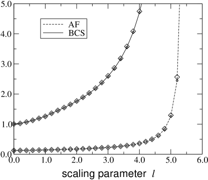
Figure 8: Comparison of results obtained from the approach of Zanchi and Schulz (circles) with those obtained when only logarithmic contributions are included (diamonds), for the case of an attractive Hubbard interaction ($U_{0}<0$) and $\mu=1$. There is no significant discrepancy between the results. Flow in the dominant BCS coupling is shown by the solid line; the AF coupling is indicated by the dashed line.

The opposite limit of a square lattice with repulsive initial interaction $U_{0}>0$ has been extensively studiedZanchi ; Halboth1 . At half-filling, the Fermi surface is perfectly nested and a strong SDW instability develops. Fig. 9 shows, however, that the largest BCS channel, though sub-leading in comparison to the SDW channel, already exhibits $d_{x^{2}-y^{2}}$ pairing symmetry.

Figure 9: Pairing symmetry of the dominant BCS channel for the case of repulsive initial interaction ($U_{0}>0$) on the square lattice ($t_{1}=1$ and $t_{2}=0$) at half-filling ($\mu=0$). The different curves correspond to different values of the scaling parameter ($\ell=0.5,1$ and $3$). The Fermi surface is divided in $M=16$ patches. As the patch index increases from $n=0$ to $n=15$ around the Fermi surface, the angle $\theta$ increases from $0$ to $2\pi$.

For the case of a repulsive Hubbard interaction, $U_{0}>0$, we find in contrast to the attractive situation that the formally irrelevant terms play an important role. As the initial BCS couplings are all repulsive, Cooper pairing can only happen via coupling to the AF channels or via the non-logarithmic corrections to scaling coming from the formally irrelevant terms in the six-point functions. We again compare RG flows which include only the leading logarithmic corrections (diamonds) against those in which all subdominant contributions at one-loop order are included (circles) in Fig. 10 for the case $\mu=10^{-4}$, that is, slightly away from half-filling. Though qualitatively similar, there is considerable quantitative difference. At this small doping, AF tendencies dominate in both cases. Upon further increasing the chemical potential, as mentioned above there is a crossover into the $d_{x^{2}-y^{2}}$ BCS regime. The crossover occurs much sooner when the subleading terms are included. Finally, at large doping the nesting of the Fermi surface is completely eliminated, and neither the AF nor the BCS channels show any strong divergences.

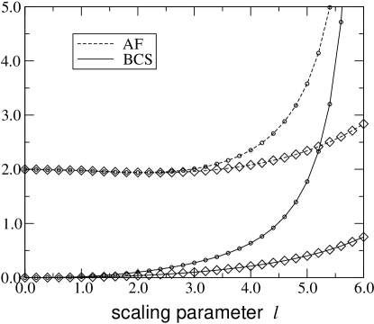
Figure 10: Comparison of results obtained at one-loop level for the case of a repulsive Hubbard interaction and $\mu=10^{-4}$. RG flows which include the effects of formally irrelevant terms (circles) are compared with RG flows for which only logarithmic contributions are retained (diamonds). Flow in the dominant BCS channel is depicted as a solid line and dominant AF sector is indicated by a dashed line.

III.3 Square Lattice With Next-Nearest-Neighbor Hopping ($t^{\prime}\neq 0$)

Next we turn to the square lattice with added next-nearest-neighbor hopping amplitude $t^{\prime}$ along each of the two diagonal directions. Weak-coupling RG studies of this Hubbard model have been carried out previously by a number of groupsHalboth1 ; Halboth2 ; Honerkamp using the formulation of Refs. Salmhofer1, ; Salmhofer2, . We have checked our calculation against these published results and find good agreement. The dispersion relation in this case is given by

$$\epsilon_{\bf k}=-2t_{1}(\cos k_{x}+\cos k_{y})-4t^{\prime}\cos k_{x}\cos k_{y}$$ (12)

and Fig. 11 show the Fermi surface for the case $t_{1}=-1$, $t^{\prime}=0.05$, and $\mu=4t^{\prime}$. The Fermi surface is centered around the $\Gamma$ point $(\pm\pi,\pm\pi)$ and van Hove singularities lie at the Fermi energyGonzalez .

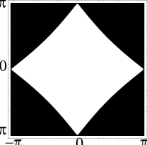
Figure 11: Fermi surface of the square lattice with nearest-neighbor hopping $t_{1}=-1$ and next-nearest-neighbor hopping $t^{\prime}=0.05$. The chemical potential $\mu=4t^{\prime}$.

This Fermi surface exhibits the $d_{x^{2}-y^{2}}$ superconducting instability. It is interesting to go a bit further and address the question of whether or not there is spontaneous time-reversal ($\hat{T}$) symmetry breaking with the appearance of an additional imaginary $id_{xy}$ component to the superconducting order parameter. To answer this question we study the implications of RG flows which yield comparable attraction in two channels: one term with $d_{x^{2}-y^{2}}$ symmetry and a second with $d_{xy}$ symmetry. A simple calculation of energetics then suffices to show that the two order parameters will phase-align as $d_{x^{2}-y^{2}}+id_{xy}$. The standard BCS equation yields a condensation energy of

$$\Delta E=E_{SC}-E_{N}=2\sum_{{\bf k}>{\bf k_{F}}}\left[\epsilon_{\bf k}-\frac{2\epsilon_{\bf k}^{2}+\Delta_{\bf k}^{2}}{2\sqrt{\epsilon_{\bf k}^{2}+\Delta_{\bf k}^{2}}}\right]\ .$$ (13)

For couplings $V^{BCS}$ with comparable $d_{x^{2}-y^{2}}$ and $d_{xy}$ components, the ansatz to maximize the condensation energy should be chosen to be $\Delta_{\bf k}=\Delta_{d_{x^{2}-y^{2}}}({\bf k})+u~{}\Delta_{d_{xy}}({\bf k})$, with $u$ encoding information about the relative phase of the two components. Substituting this ansatz into Eq. 13, we may then determine the phase that maximizes the condensation energy $\Delta E$. Fig. 12 shows the dependence of the sum

$$I(u)=\sum_{{\bf k}>{\bf k_{F}}}{2\epsilon_{\bf k}^{2}+\Delta_{\bf k}^{2}\over\sqrt{\epsilon_{\bf k}^{2}+\Delta_{\bf k}^{2}}}$$ (14)

on the real part of $u$. This term is maximized when $u$ is purely imaginary (Re$\{u\}=0$), hence the $\hat{T}$-breaking pairing symmetry $d_{x^{2}-y^{2}}+id_{xy}$ is the energetically favored. Physically this is reasonable, as this choice of the phase guarantees that a gap forms everywhere along the Fermi surface, lowering the ground-state energy.

Figure 12: Dependence of the integral $I(u)$ on the real part of $u$. The maximum of $I(u)$ occurs when Re$\{u\}=0$, that is, when $u$ is purely imaginary.

Returning to the square lattice, we find that upon integrating the RG equations for the case $t_{1}=-1$, $t^{\prime}=0.05$ and $\mu=4t^{\prime}$, the dominant attractive BCS channel has $d_{x^{2}-y^{2}}$ symmetry as expected; see Fig. 13(A). A channel with $d_{xy}$ symmetry also appears but it is repulsive in sign; see Fig. 13(B).

Figure 13: Dominant BCS channels for the square lattice with $t_{1}=-1$, $t^{\prime}=0.05$ and $\mu=4t^{\prime}$, at scaling parameter $\ell=5$. The $d_{x^{2}-y^{2}}$ channel (A) is attractive while the $d_{xy}$ channel (B) is repulsive. The absolute values of the eigenvalues are plotted in Fig. 14 as functions of the scaling parameter $\ell$.

The strengths of each channel are plotted in Fig. 14 as a function of the scaling parameter $\ell$. Since the $d_{xy}$ channel is repulsive, no $d_{xy}$ order will arise, and this may be taken as evidence against the formation of spontaneous time-reversal symmetry breaking of the $d_{x^{2}-y^{2}}+id_{xy}$ type.

Figure 14: Flow of the eigenvalues for the $d_{x^{2}-y^{2}}$ and $d_{xy}$ channels shown in Fig. 13. The magnitude of the eigenvalues is plotted.

III.4 Towards the Triangular Lattice ($t_{2}\neq 0$, $t_{2}<t_{1}$)

Introducing non-zero $t_{2}$ along just one of the two diagonals, as shown in Fig. 1, offers a different way of breaking-up perfect nesting and enhancing BCS instabilities, even at half-fillingTsai . For sufficiently large $t_{2}$ there is a crossover to a regime where the BCS processes eventually dominate, signaling a superconducting instability. Furthermore, because the Fermi surface is imperfectly nested, the growth of both BCS and AF couplings weakens. Further increasing $t_{2}$ eventually destroys nesting of the Fermi surface altogether and both types of divergences are suppressed. Three cases illustrating the crossover are shown in Fig. 15.

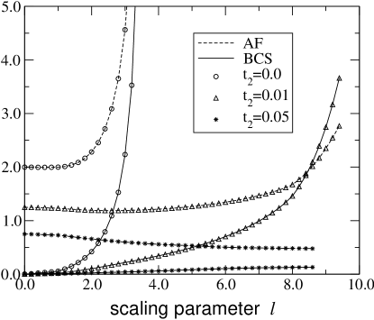
Figure 15: At half-filling, spin-wave instability occurs for $t_{2}=0$, but as $t_{2}$ increases, the BCS instability wins over. This is due to imperfect nesting. As $t_{2}$ is increased further, the nesting is destroyed and both divergences are suppressed. The hopping $t_{1}$ is chosen such that $t_{1}+t_{2}=1$.

As further increases in the diagonal hopping $t_{2}$ suppress the $d_{x^{2}-y^{2}}$ BCS channel, this channel diminishes relative to other subdominant BCS channel with different symmetries, for example d_xy- or p-wave, as shown in Fig. 16. These other channels, however, are all repulsive and hence do not lead to BCS instabilities by themselves.

Figure 16: Dominant BCS channels for $t_{1}=0.9$ and $t_{2}=0.1$, at half-filling and at scaling parameter $\ell=5$. These channels are both repulsive (with eigenvalues of 0.19525 and 0.162 respectively). The attractive $d_{x^{2}-y^{2}}$ BCS channel has a small eigenvalue of -0.268.

We note that the Hubbard model on the anisotropic triangular lattice has also been studied using the the random-phase approximationVojta and the fluctuation-exchange (FLEX) approximationKondo ; Kino ; Schmalian . The $d$-wave superconducting instability was found to be dominant for a large range of values of $t_{2}/(t_{1}+t_{2})$ interpolating between the square lattice and the isotropic triangular lattice.

III.5 Isotropic Triangular Lattice At Half-Filling

For the special case of the isotropic triangular lattice ($t_{1}=t_{2}=0.5$) at half-filling, the weak-coupling RG flows do not show any BCS instabilities. The dominant BCS channels, $d_{x^{2}-y^{2}}$, $d_{xy}$ and $p$, are all repulsive. These channels are depicted in Fig. 17(A), 17(B) and 17(C).

Figure 17: BCS channels for the isotropic triangular lattice $t_{1}=t_{2}=0.5$, at scaling parameter $\ell=8.4$. Channels with $d_{x^{2}-y^{2}}$ (A), $d_{xy}$ (B) and $p$ (C) symmetries all appear as repulsive channels (with eigenvalues 0.0378, 0.035 and 0.057, respectively). The largest attractive BCS channel is shown in (D), but it has a very small coefficient (-0.020) and the rapid oscillations suggest that the calculation is not accurate at this point. In the calculation, the Fermi surface was divided into $M=24$ patches, instead of just 16, to improve the accuracy in the higher wave channels.

Fig. 17(D) shows the first attractive channel that develops, but the rapid oscillations in the effective potential, and its small size, indicate that the calculation is not reliable.

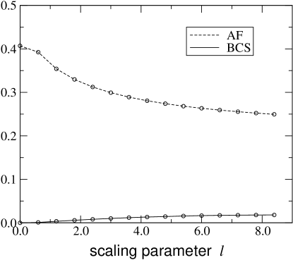
Figure 18: Flow of dominant AF and BCS channels for the case of the isotropic triangular lattice.

In Fig. 18 the dominant AF and BCS channels are compared. Neither channel shows strong divergences, but the AF channel is significantly larger than the BCS channel. Thus there are signs of re-entrant antiferromagnetic long-range order. We speculate that there exist four different regions as the isotropy parameter $t_{2}/(t_{1}+t_{2})$ changes form $0$ (square lattice) to $1$ (decoupled chains). These phases are shown in Fig. 19. At $t_{2}=0$ the system exhibits long-range antiferromagnetic Néel order (LRO) with ordering vector $\vec{Q}=(\pi,\pi)$. But this long-range order is suppressed by turning on $t_{2}$. Instead $d_{x^{2}-y^{2}}$ BCS instabilities dominate and only short-range order (SRO) occurs. Both AF and BCS instabilities are suppressed as $t_{2}$ is further increased and the nesting is completely eliminated. Nevertheless, the AF coupling remains significantly larger than the BCS coupling. In the strong-coupling limit $U\rightarrow\infty$ the model can be mapped onto a nearest-neighbor spin-1/2 Heisenberg antiferromagnet which of course is insulating. On the isotropic triangular lattice this antiferromagnet exhibits long-range AF orderSingh ; Bernu with ordering wave vector $\vec{Q}=(4\pi/3,0)$. The question of whether or not our weak-coupling analysis can describe this strong-coupling limit is tantamount to asking whether or not one or more intermediate-coupling fixed points intervene between the repulsive weak-coupling fixed point that is accessible in our RG analysis, and the attractive strong-coupling fixed point which describes the antiferromagnetic insulator. Finally as $t_{2}$ becomes larger than $t_{1}$, the chains begin to decouple. In the extreme limit of independent chains there can be no long-range spin order, as the Mermin-Wagner theorem tells us that continuous symmetries cannot break in 1+1 dimensions.

Figure 19: Four regions of the $U>0$ phase diagram, LRO / SRO / LRO / SRO, identified as $t_{2}/(t_{1}+t_{2})$ varies from $0$ (square lattice) to $1$ (decoupled chains).

Curiously, four such regions, LRO / SRO / LRO / SRO, have also been identified in the corresponding strong-coupling Heisenberg antiferromagnet with two exchange couplings $J_{1}$ and $J_{2}$. The phase diagram of this model has been studied via a straightforward $1/S$ expansionMerino ; Trumper , a series expansion methodWeihong , and a large-$N$ Sp(N) solutionChung . All three methods find two regions of long-range order: near the limit of a square lattice ($J_{2}=0$) and near the isotropic point ($J_{2}=J_{1}$). It is remarkable that our weak-coupling RG analysis shows similar behavior.

The Hubbard model on the triangular lattice has been studied at intermediate values of the interaction strength within the Hartree-Fock approximationKrishnamurthy ; Jayaprakash and within the slave-boson methodGazza ; Feiguin ; Capone . A Mott-Hubbard metal-insulator transition is found to occur at a relatively large value of $U_{c}$ ($U_{c}=5.27t$ for the Hartree-Fock calculationKrishnamurthy and $U_{c}=7.23t$ or $7.68t$ from the slave-boson calculationsGazza ; Capone ). At a smaller value of $U=U_{c1}$ there is also a continuous transition from a paramagnetic metallic phase to a metallic phase with incommensurate spiral order. The Hartree-Fock calculation yields $U_{c1}=3.97t$ and the slave-boson calculation gives $U_{c1}=6.68t$ for this transition. Signs of re-entrant AF order in our weak-coupling RG calculation, namely the relatively large size of the AF channels in comparison with the BCS channels, are broadly consistent with this picture, as AF tendencies can be a precursor to a transition to the insulating state.

IV Conclusion

Hubbard models have received extensive study in the context of high-$T_{c}$ superconductivity. We have reproduced the well-known result that there is an AF instability at half-filling on the square lattice with repulsive on-site Coulomb interaction and nearest-neighbor hopping. Furthermore, upon doping the system away from half filling, a crossover to a BCS regime with $d_{x^{2}-y^{2}}$ pairing symmetry occurs as expected. We have shown that it is important to retain subleading, formally irrelevant, corrections to the RG flows when the bare interaction is repulsive and the Fermi surface is nearly nested. We also studied another way of triggering a BCS instability. Keeping the system at half filling, but introducing the diagonal hopping $t_{2}$ as shown in Fig. 1 along one of the two diagonals, breaks up perfect nesting. Corresponding magnetic frustration kills the spin density wave, and Cooper pairing dominates, at least if $t_{2}$ is not too large. This result suggests that superconductivity can occur in a model of strongly correlated electrons, even at half-filling. We emphasize that stripes are not expected to play a role here; even moderate on-site Coulomb repulsion should inhibit charge segregation at half-filling.

The half-filled Hubbard model on the anisotropic triangular lattice has been proposed as a minimal description of the conducting layers of the $\kappa$-(BEDT-TTF)₂X organic superconductors. It is important to establish the pairing symmetry of the superconducting state of these materials. Our theoretical results predict pairing of the $d_{x^{2}-y^{2}}$ type and in fact signs of such order have been seen experimentally. We did not find any evidence of spontaneous time-reversal symmetry breaking. Pairing symmetry of the type $d_{x^{2}-y^{2}}\pm id_{xy}$ would occur if an attractive $d_{xy}$ channel arose in addition to the $d_{x^{2}-y^{2}}$ channel. We find that attractive $d_{xy}$ channels neither occur when next-nearest-neighbor hopping $t^{\prime}$ is included on the square lattice, nor when non-zero hopping $t_{2}$ is turned on along one of the two diagonal directions.

Finally, we made contact with previous work on Heisenberg antiferromagnets on the anisotropic triangular lattice. Our weak-coupling RG calculation shows AF tendencies in two separate regimes – tendencies which seem to correspond with the two AF ordered phases found previously at large-$U$. In particular the portion of the phase diagram between the isotropic point ($t_{1}=t_{2}$) and decoupled chains ($t_{1}=0$) is the relevant region for the layered Cs₂CuCl₄ antiferromagnet insulator material. The competition we found between antiferromagnetic order and spin-liquid behavior in our RG calculation may be consistent with the observed ease by which spin order is destroyed in the compoundRadu .

Acknowledgments We thank Chung-Hou Chung, Tony Houghton, Ross McKenzie, and Matthias Vojta for useful discussions. This work was supported in part by the NSF under Grant Nos. DMR-9712391 and DMR-0213818.

References

- (1) J. M. Williams et al. 1992 Organic superconductors (including fullerenes): synthesis, structure, properties, and theory, (Englewood Cliffs: Prentice Hall)
- (2) T. Ishiguro and K. Yamaji 1997 Organic Superconductors, Second edition (Berlin: Springer-Verlag)
- (3) R. H. McKenzie 1998 Comments Cond. Mat. Phys. 18 309
- (4) R. H. McKenzie 1997 Science 278 820.
- (5) H. Mayaffre, P. Wzietek, D. Jérome, C. Lenoir and P. Batail 1995 Phys. Rev Lett. 75 4122
- (6) S. M. De Soto, C. P. Slichter, A. M. Kini, H. H. Wang, U. Geiser and J. M. Williams 1995 Phys. Rev. B 52 10364
- (7) K. Kanoda, K. Miyagawa, A. Kawamoto and Y. Nakazawa 1996 Phys. Rev. B 54 76
- (8) Y. Nakazawa and K. Kanoda 1997 Phys. Rev. B 55 R8670
- (9) K. Kanoda, K. Akiba, K. Suzuki, T. Takahashi and G. Saito 1990 Phys. Rev. Lett. 65 1271
- (10) L. P. Le, G. M. Luke, B. J. Sternlieb, W. D. Wu, Y. J. Uemura, J. H. Brewer, T. M. Riseman, C. E. Stronach, G. Saito, H. Yamochi, H. H. Wang, A. M. Kini, K. D. Carlson and J. M. Williams 1992 Phys. Rev. Lett. 68 1923
- (11) D. Achkir, M. Poirier, C. Bourbonnais, G. Quirion, C. Lenoir, P. Batail and D. Jérome 1993 Phys Rev B 47 11595
- (12) A. Carrington, I. J. Bonalde, R. Prozorov, R. W. Giannetta, A. M. Kini, J. Schlueter, H. H. Wang, U. Geiser and J. M. Williams 1999 Phys. Rev. Lett. 83 4172
- (13) M. Pinterić, S. Tomić, M. Prester, D. Drobac, O. Milat, K. Maki, D. Schweitzer, I. Heinen and W. Strunz 2000 Phys. Rev. B 61 7033
-
(14)
T. Arai, K. Ichimura, K. Nomura, S. Takasaki, J. Yamada,
S. Nakatsuji and H. Anzai 2001 Phys. Rev. B 63 104518
T. Arai, K. Ichimura, K. Nomura, S. Takasaki, J. Yamada, S. Nakatsuji and H. Anzai 2000 Solid State Comm. 116 679 -
(15)
J. M. Schrama, E. Rzepniewski, R. S. Edwards, J. Singleton,
A. Ardavan, M. Kurmoo and P. Day 1999 Phys. Rev. Lett 83 3041
J. M. Schrama and J. Singleton 2001 Phys. Rev. Lett 86 3453 - (16) S. Hill, N. Harrison, M. Mola, J. Wosnitza 2001 Phys. Rev. Lett. 86 3451
- (17) T. Shibauchi, Y. Matsuda, M. B. Gaifullin, T. Tamegai 2001 Phys. Rev. Lett. 86 3452
- (18) S. Belin, K. Behnia, A. Deluzet 1998 Phys. Rev. Lett. 4728
- (19) K. Izawa, H. Yamaguchi, T. Sasaki, Y. Matsuda 2002 Phys. Rev. Lett. 88 027002
- (20) D. R. Harshman, R. N. Kleiman, R. C. Haddon, S. V. Chichester-Hicks, M. L. Kaplan, L. W. Rupp Jr., T. Pfiz, D. L. Williams and D. B. Mitzi 1990 Phys. Rev. Lett. 64 1293
- (21) O. Klein, K. Holczer, G. Grüner, J. J. Chang and F. Wudl 1991 Phys. Rev. Lett. 66 655
-
(22)
M. Lang, N. Toyota, T. Sasaki and H. Sato 1992
Phys. Rev. Lett. 69 1443
M. Lang, N. Toyota, T. Sasaki, and H. Sato 1992 Phys. Rev. B 46 5822 - (23) D. R. Harshman, A. T. Fiory, R. C. Haddon, M. L. Kaplan, T. Pfiz, E. Koster, I. Shinkoda and D. Ll. Williams 1994 Phys. Rev. B 49 12990
- (24) M. Dressel, O. Klein, G. Grüner, K. D. Carlson, H. H. Wang and J. M. Williams 1994 Phys. Rev. B 50 13603
- (25) H. Elsinger, J. Wosnitza, S. Wanka, J. Hagel, D. Schweitzer and W. Strunz 2000 Phys. Rev. Lett. 84, 6098 (2000)
- (26) S. Lefebvre, P. Wzietek, S. Brown, C. Bourbonnais, D. Jérome, C. Mézière, M. Fourmigué and P. Batail 2000 Phys. Rev. Lett. 85 5420
-
(27)
R. Coldea, D. A. Tennant, A. M. Tsvelik, and Z. Tylcznski,
2001 Phys. Rev. Lett. 86 1335
R. Coldea, D. A. Tennant, K. Habicht, P. Smeibidl, C. Wolters, and Z. Tylcznski 2002 Phys. Rev. Lett. 88 137203
R. Coldea 2003 (private communication) - (28) K. Takada, H. Sakurai, E. Takayama-Muromachi, F. Izumi, R. A. Dilanian, and T. Sasaki, 2003 Nature 422 53
- (29) R. J. Balsys and R. L. Davis 1996 Solid State Ionics 93 279
- (30) H. Kino and H. Fukuyama 1996 J. Phys. Soc. Jpn. 65 2158
- (31) E. H. Lieb and F. Y. Wu 1968 Phys. Rev. Lett. 20 1145
- (32) E. S. Choi, J. S. Brooks, S. Y. Han, L. Balicas and J. S. Qualls 2001 Philos. Mag. B 81 399
-
(33)
D. Zanchi and H. J. Schulz 1998 Europhys. Lett. 44
235
D. Zanchi and H. J. Schulz 2000 Phys. Rev. B 61 13609 - (34) See, for example, A. Houghton, H.-J. Kwon, and J. B. Marston 2000 Adv. Phys. 49 141 and references therein
- (35) R. Shankar 1994 Rev. Mod. Phys. 66 129
- (36) S. Dusuel, F. Vistulo de Abreu, and B. Doucot 2002 Phys. Rev. B 65 94505
- (37) D. Zanchi and H. J. Schulz 1996 Phys. Rev. B 54 9509
- (38) M. Salmhofer 1998 Comm. Math. Phys. 194 249
- (39) M. Salmhofer 1999 Renormalization: An Introduction, (Berlin: Springer-Verlag)
- (40) C. J. Halboth and W. Metzner 2000 Phys. Rev. B 61 7364
- (41) C. J. Halboth and W. Metzner 2000 Phys. Rev. Lett. 85 5162
- (42) C. Honerkamp, M. Salmhofer, N. Furukawa and T. M. Rice 2001 Phys. Rev. B 63 035109
- (43) H. H. Lin, L. Balents, and M. P. A. Fisher 1998 Phys. Rev. B58, 1794
- (44) J. O. Fjærestad and J. B. Marston 2002 Phys. Rev. B 65, 125106.
- (45) J. B. Marston, J. Fjærestad, and A. Sudbø 2002 Phys. Rev. Lett. 89, 056404
- (46) I. Affleck 1990 in Fields, Strings and Critical Phenomena, edited by E. Brezin and J. Zinn-Justin (Amsterdam: North-Holland)
-
(47)
J. González and M. A. H. Vozmediano 2000
Phys. Rev. Lett. 84 4930
J. González 2001 Phys. Rev. B 63 45114 - (48) S.-W. Tsai and J. B. Marston 2001 Can. J. Phys. 79 1463
- (49) M. Vojta and E. Dagotto 1999 Phys. Rev. B 59 R713
- (50) H. Kondo and T. Moriya 1998 J. Phys. Soc. Jpn. 67 3695
- (51) H. Kino and K. Kontani 1998 J. Phys. Soc. Jpn. 67 3691
- (52) J. Schmalian 1998 Phys. Rev. Lett. 81 4232
- (53) R. R. P. Singh and D. Huse 1992 Phys. Rev. Lett. 68 1766
- (54) B. Bernu, P. Lecheminant, C. Lhuillier and L. Pierre 1994 Phys. Rev. B 50 10048
- (55) J. Merino, R. H. McKenzie, J. B. Marston and C.-H. Chung 1999 J. Phys.: Condens. Matter 11 2965
- (56) A. E. Trumper 1999 Phys. Rev. B 60 2987
- (57) Z. Weihong, R. H. McKenzie and R. R. P. Singh 1999 Phys. Rev. B 59 14367
- (58) C. H. Chung, J. B. Marston and R. H. McKenzie 2001 J. Phys.: Condens. Matter 13 5159
- (59) H. R. Krishnamurthy, C. Jayaprakash, S. Sarker and W. Wenzel 1990 Phys. Rev. Lett. 64 950
- (60) C. Jayaprakash, H. R. Krishnamurthy, S. Sarker and W. Wenzel 1991 Europhys. Lett. 15 625
- (61) C. J. Gazza, A. E. Trumper and H. A. Ceccato 1994 J. Phys.: Condens. Matter 6 L625
- (62) A. Feiguin, C. J. Gazza, A. E. Trumper and H. A. Ceccato 1997 J. Phys.: Condens. Matter 9 L27
- (63) M. Capone, L. Capriotti, F. Becca and S. Caprara 2001 Phys. Rev. B 63 085104