Recurrent oligomers in proteins – an optimal scheme reconciling accurate and concise backbone representations in automated folding and design studies

Abstract

A novel scheme is introduced to capture the spatial correlations of consecutive amino acids in naturally occurring proteins. This knowledge-based strategy is able to carry out optimally automated subdivisions of protein fragments into classes of similarity. The goal is to provide the minimal set of protein oligomers (termed “oligons” for brevity) that is able to represent any other fragment. At variance with previous studies where recurrent local motifs were classified, our concern is to provide simplified protein representations that have been optimised for use in automated folding and/or design attempts. In such contexts it is paramount to limit the number of degrees of freedom per amino acid without incurring in loss of accuracy of structural representations. The suggested method finds, by construction, the optimal compromise between these needs. Several possible oligon lengths are considered. It is shown that meaningful classifications cannot be done for lengths greater than 6 or smaller than 4. Different contexts are considered were oligons of length 5 or 6 are recommendable. With only a few dozen of oligons of such length, virtually any protein can be reproduced within typical experimental uncertainties. Structural data for the oligons is made publicly available.

I Introduction

One of the most fundamental and still unsolved problems in biology is the elucidation of the folding process, that is how a protein sequence undergoes the structural rearrangements that eventually lead to the biologically active conformation (believed to be the free energy minimum) [1]. Since the early studies of Levinthal it was clear that the dynamics of folding to the native state could not be governed by mere random processes [2]; indeed modern folding theories explain fast folding processes by invoking nucleation-condensation mechanisms or funnel-like energy landscapes [3, 4] that dramatically reduce the space of visited conformations [5, 6, 7, 8]. Topologic, steric and chemical features are so effective in reducing the space of viable conformations that even at a local level, only few degrees of freedom per amino acid are observed. This fact, originally observed by Ramachandran [9] has been lately used in a variety of numerical schemes. In these approaches proteins are modeled as chains of one or two interacting centers (representing individual amino acids) with a limited set of local degrees of freedom, such as torsion angles or Cartesian positions, chosen to provide optimal compromises between accurate representation and number of degrees of freedom [10, 11, 12]. These models appear excellent from many points of view with the exception that they fail to capture correlations between torsion angles along the peptide chain.

In this paper we address this problem and propose an optimal way to extend the original idea of Ramachandran of limiting the degrees of freedom of individual residues to strings of consecutive amino acids, showing that they are far from independent. Indeed, their correlations are so strong that, as originally pointed out in a paper by Alwyn Jones and Thirup [13], it is possible to construct a small data bank of protein fragments that can be used as elementary building blocks to reconstruct virtually all native protein structures. We start by following the seminal idea of Unger et al. [14] that oligomers of a given length found in a coarse grained representation (such as $C_{\alpha}$ coordinates) of native structures do not vary continuously but they gather in few clusters. Each of these can be represented by a single element (that we term “oligon”) that optimally catches the geometrical and topological properties of the entire basin.

Our approach differs from previous work on the classification of structural fragments [14, 15, 16] in that the procedure we follow to select the oligons has been explicitly optimised for use in fully automated contexts, especially folding and design attempts [8, 17, 18, 19, 21, 22, 23, 24, 25, 26, 27]. Indeed, such attempts are commonly framed within numerical problems of minimizing suitable functionals (such as energy scoring functions) in structure space. The addition of local constraints reduces drastically the space of viable structures and is undoubtedly a desired feature allowing to keep to a minimum the side-effects of using imperfect parametrizations of the free energy or imperfectly known interaction potentials [28, 29, 30, 31, 32, 33, 34, 35, 36, 37, 38].

The selection strategy we propose is free of subjective inputs or biases and exploits the full knowledge-based information intrinsic in our data-bank of non-redundant protein structures. An appealing feature of the suggested method is that representative fragments are singled out in order of importance, that is according to the frequency in which they appear in natural proteins. We carry out a series of thorough checks and validations of the clustering strategy and show that the optimal sets of oligons do not suffer from finite-size effects of the data bank. It is shown that the optimal representatives have length equal to 5 or 6 and that with only a few tens of them it is possible to fit virtually any protein within about 1.0 Å co-ordinate root mean square deviations (cRMS) per amino acid. Some of the ramifications of this study are discussed and outlined through preliminary investigations in Section III. The optimal sets of oligons presented and discussed here are made publicly available at http://www.sissa.it/~michelet/prot/repset.

II Methods and Results

The first step in the creation of a set of optimal representatives is the set up of a sufficiently large data bank of protein structures. Such data bank should cover as best as possible the variety of distinct protein structures observed in nature. At the same time it is important to eliminate correlations and biases in the data bank resulting, for example, from structural homology [39] For these reasons we compiled our data bank by choosing 75 single-chain proteins from a carefully compiled list of non-redundant structures [37].

The proteins, listed in Table I were chosen from the SCOP database of non-redundant single-chain proteins covering the most common families: all $\alpha$, all $\beta$, $\alpha\beta$ and $\alpha+\beta$ and the most common chain lengths. This ensures that, a priori, the selected structures represent a broad spectrum of structural instances with the least bias or redundancy. As discussed later, the results confirm a posteriori, that the size and quality of the data-bank was sufficient for all practical purposes. Each of the proteins of Table I was partitioned in all the possible fragments of $l$ consecutive residues. We considered values of $l$ ranging from 3 to 10, for which there are 10936 to 10411 distinct fragments. As in previous studies involved with structural classifications, we retained only the $C_{\alpha}$ coordinates of each fragment [14, 15, 16, 40].

This approach, is practical and consistent with the idea of having an optimal, but schematic representation of structures. Moreover it is “reversible” to a great extent since the whole peptide atomic geometry can be recovered from the mere knowledge of $C_{\alpha}$ co-ordinates [42]. In turn, if needed, optimal side-chain rotamer positions could be satisfactorily obtained by exhaustive or stochastic methods [22, 27].

A Theory: clustering algorithm

The goal pursued in this work is to provide a synthetic, but exhaustive, classification of inequivalent local structural motifs to be used in contexts where a broad exploration of the space of viable protein structures is concerned. Hence, the approach pursued here differs from studies aimed at selecting a restricted number of motif classes to be used in homology modelling or automated recognition/classification of secondary motifs [14, 15, 16, 40, 41, 44, 45, 46]. This distinct goal is accordingly pursued with a novel strategy for the identification of classes that is reminiscent of the clustering technique used by Lacey and Cole in an unrelated context [47]. In the following we shall try to propose a strategy able to perform an optimal subdivision into classes of similarity and, for each of these, provide the best representative. Two of the points of force of such method are the absence of any subjectivity or human supervision through the extensive use of optimal knowledge-based classification criteria and also the fact that similarity classes are automatically extracted and ranked according to their frequency of appearance in natural proteins. This wealth of knowledge-based information provided by the procedure allows to choose the representative set that best matches one’s needs. The clustering procedure we used to partition the fragments in suitable similarity classes is conveniently illustrated by the two-dimensional example of Fig. 1 where 1000 points have been assigned randomly to 4 distinct clusters with the same radius but different size (i.e. number of members). Considerable information about the clusters can be obtained by analyzing the histogram of the distance between all pairs of members in the set. At the simplest level the histogram analysis can reveal two distinct scenarios: a) no clusters are present or b) there are clusters with comparable size and degree of internal similarity. In the first case the histogram distribution is expected to crowd around an average value in a bell-shaped fashion. In the second case, two distinct peaks should occur: one corresponding to the typical distance within classes, the other centered around the (larger) average distance of pairs of members from distinct classes. In the case of very few [many] classes, the first [second] peak dominates.

The inset of Fig. 1 shows the pair-distance histogram for the set of points in our example. It is evident that it consists of two peaks: the first one extends till about the radius of clusters while the location of the second peak coincides with the typical cluster-cluster distance.

Our goal is to exploit the information obtained from the pair-distance histogram to identify first how many different clusters there are and secondly the optimal representative of each cluster. To do so we follow the intuitive expectation that the best representative of each cluster is the one closest to the cluster center. A deterministic way to identify the center of homogeneous clusters, is to find the member with the largest number of other points within a suitably chosen similarity cutoff (we shall term this number “proximity score”). Indeed, points further from the center will have fewer neighbors. This “election” mechanism is reliable for large and homogeneous clusters.

Hence, we start by choosing the first representative of the set as the one with the highest proximity score. This identifies simultaneously both the largest cluster and its representative. Next, we remove the representative and its cluster from the set and recalculate the proximity score of the remaining points and again we select the member with the highest score. As before we removed it and its cluster and proceed in this iterative fashion until the set of surviving points is exhausted.

When such scheme is applied to the set of Fig. 1 – using a similarity cutoff equal to $R$=1 – the optimal representatives of the four clusters (marked with squares) are immediately found and ranked according to their cluster size.

B Results

We applied the same scheme to analyze our data bank of thousands of protein fragments. This time, the points of the previous example are replaced by the fragments themselves, while the notion of eucledian distance between two points is substituted by the cRMS distance of two fragments [14], $X$ and $Y$ of equal length, $N$,

$$\sigma(X,Y)=\sqrt{\sum_{k=1}^{N}\left|\vec{r}^{C_{\alpha}}_{k}(X)-\vec{r}^{C_{\alpha}}_{k}(Y)\right|^{2}\over N}\ .$$ (1)

This notion of distance is meaningful provided that $X$ and $Y$ have been previously optimally superimposed with the standard Kabsch procedure [48] . The calculation of the cRMS of each distinct pair of fragments is the most computationally demanding step since it requires an application of the Kabsch algorithm [48] for each distinct pair of fragments (e.g. this translates in well over ten million pairs of fragments for lengths of the order of 5).

The histogram of all cRMS of pairs of fragments of lengths in the range $3\leq l\leq 10$ is given in Fig. 2. It can be seen that all distributions show two distinct peaks, with the exception of $l=3$, which appears to be exceptionally short, and hence will be omitted from further analysis.

For the smaller lengths, the first peak collects a substantial amount of “hits”, proving that it is meaningful to assume the presence of classes of similarity. It also appears that the height of the first peak constantly decreases with increasing $l$. This confirms the intuition that, by considering very large values of $l$ every fragment will be a class for itself. Indeed, for lengths greater than 6, the first peak is hardly discernible from the background. Hence, the mere visual inspection of histogram distributions shows that it would not be justifiable to force the introduction of classes of similarity for lengths above 6. Nevertheless, we shall often present results also for length 7 for the purpose of showing how several unrelated criteria indicate such length as a border-case of viable oligons. An important observation for our subsequent analysis is that the extension of the first peak (the intra-cluster one) depends only weakly on $l$ and is about 0.65 Å. This provides an unbiased measure for the similarity cutoff and hence we adopted it. The location of the second “background” peak in the histogram of Fig. 2 gives an estimate of the similarity between unrelated fragments and, hence, crresponds to the cRMS deviation of a random pair of segments. This random pair distance increases with the chain length, but it always well above the value of 2 Å, thus justifying a posteriori the use of similarity cutoffs of the order of 1 Å   considered in previous studies [14, 40].

The advantage of the clustering scheme introduced and used here is that, with modest computational effort (the cRMS distances need to be computed once for all) one has simultaneously both the subdivision in clusters and their optimal representatives. An extra payoff of this approach over other clustering schemes is that the representatives are singled out in order of importance. It is important to stress that there is no stochastic element in the analysis since the assignement of elements to clusters follows a “greedy” deterministic approach. One particular instance where the suggested strategy may fail, is when the “fringes” of distinct clusters overlap, that is when an element falls in the similarity basin of more than one representative. In this situation, more sophisticated clustering techniques (such as those based on k-means analysis [20]) ought to be adopted in place of the present one, in fact, the iterative removal of assigned members would affect both the choice of the representative and also its score. Although we cannot rule out the presence of fringe overlaps in our data bank, we can exclude it has any substantial significance. Indeed, we have checked that the typical cRMS of the extracted representatives matches the random pair distance which, being much greater than 0.65 Å, makes overlaps highly improbable.

Our analysis identified only 28 representatives for length $l=4$, 202 for $l=5$, 932 for $l=6$ and 2561 for $l=7$. As we mentioned before, the existence of a limited repertoire of local folds is a consequence of the existence of a discrete number of degrees of freedom per amino acids, as pointed out by the seminal studies of Levitt on $n$-state models [11]. The results obtained here contain significantly more knowledge-based information since, for instance, they also yield the representation score of each representative. It appears that the representation weight (i.e. proximity score) of the fragments decreases very rapidly with the rank (see Fig. 3 and Table II). This is an extremely important feature since it indicates that one might discard the representatives with negligible score and hence work with a subset of the whole data bank. This issue is examined in the next section.

One may expect that the best representatives should belong to the most common structural motifs such as helices, strands or turns, whereas the less frequent ones should correspond to the atypical parts of proteins (structure exceptions). This expectation is confirmed by inspection of the actual shape of the highest ranking fragments; the consensus with the work of [15, 16] and Unger [14] shows the reliability with which the main motifs can be identified in different contexts or with different methods. The first four oligons for $l=5$ and $l=6$ are shown in Figs. 4 and 5 (the structural data for the complete sets is available at the URL given in the introduction). The native environment of the first ten fragments of length 5 and 6 are given in Table II. For $l=5$ we have also shown the native environments of the best representatives in Fig. 6. A striking outcome of the clustering analysis is that the first 15 oligons of length 5 and 6 represent over 75 % and 47 %, respectively, of the whole data-bank fragments! To the best of our knowledge, this are the smallest sets of representative fragments able to cover most local structural instances with an uncertainty comparable with the best experimental resolution.

III Discussion

A Analysis of the clustering procedure

Before testing the goodness of the representative fragments it is necessary to validate the clustering procedure and ensure that the results are robust and not too dependent on the details of the data bank. We carried out a first check by studying how the outcome of the clustering scheme is affected by the size of our data bank. To be precise, this test goes beyond the mere validation of the oligon extraction scheme, since it also constitutes a check of the applicability of any clustering scheme to protein fragments. To proceed in an unbiased way we randomized the order of fragments in the data bank, so to cancel correlations of consecutive (overlapping) oligons, and extracted the representatives for an increasing number of fragments taken from the top of the randomized list. A careful analysis of the data has revealed that, for any length, $l$, the number of trivial representatives, i.e. those that, having score equal to 1, represent only themselves, grows linearly with the size of the data bank. The preportion of trivial representatives is about 0.5 %, 2% of the whole population for lengths 5, 6. For length greater than 6 the proportion of trivial representatives is considerable (being greater than 10 %). On the other hand, for $4\leq l\leq 6$ the number of non-trivial representatives shows very little increase with the size of the data bank and can be considered constant for all practical purposes. This provides a solid a posteriori confirmation that the data-bank is of sufficiently large size. Of course, the number of representatives and their growth with data-bank size depends on the particular choice of similarity cutoff (the smaller the value, the larger the number of classes). In this particular study the choice of the cutoff was dictated by the properties of the very same data to be clustered. Nevertheless, the use of physically viable cutoffs lead, invariably, to the identification of the same high-ranking clusters and, correspondingly, almost identical representatives. This could be expected a priori since identifying the most common local folds should be independent, to a large extent, on the details of the clustering procedure. As explained in the next sectiom, we tried to build on this robust result and concentrate only on the top representatives.

B Reducing the representative sets

Since the trivial oligons mentioned in Sec. III A represent only themselves, one may wonder if they can be dropped from the set and still be able to represent well the majority of native structures. In this subsection we considered this problem and try to quantify the attainable accuracy in representation when a subset of the representatives is used. For a preassigned number, $m$, of representatives to be used, the optimal accuracy is obtained when the $m$ highest ranking fragments are taken. Hence, our extraction scheme is particularly convenient for this type of study since it yields the representative fragment ranked according to their proximity score

In this framework, we measure the accuracy of representation by the amount of local structural deformation required to bring all fragments of the native structure within the proximity basin of any of the reduced oligons (while in Sect. IIID we shall fit several proteins with the oligons). This is a sort of measure of the “completeness” of the set of oligons: if the used set of oligons represented all possible instances of protein fragments, no deformation would be required. On the contrary, the poorer the set of representatives, the larger is the deformation required to bring the original fragments in the proximity basin of one oligon. To do so, we use a stochastic Monte Carlo dynamics on the backbone (described in Appendix A) to minimise the following quantity:

$$S\equiv\sum_{i=0}^{L/l-1}(\sigma(B_{i},\omega_{i})-R)^{2}\cdot\theta[\sigma(B_{i},\omega_{i})-R]$$ (2)

where $L$ is the length of the protein, $\sigma$ is the cRMS distance of eqn. 1, $B_{i}$ is the $i$th backbone fragment of length $l$, $\omega$ is its closest oligon, R is the similarity distance (0.65 Å) and $\theta$ is the usual step function.

By using the stochastic dynamics, the starting structure is deformed until all fragments are within the preassigned distance R from one of the oligons. When this happens, the score function, $S$, is exactly zero and the dynamics is stopped. By measuring how far (in terms of cRMS) the backbone has moved from its original position we can judge whether the achievable quality of representation is acceptable. We carried out this scheme by using only the first few representatives (for each length $4\leq l\leq 7$ ) and then increased their number progressively (always choosing the highest ranking ones). The cRMS as a function of the number of representatives is shown in Figs. 7. For $4\leq l\leq 6$ only a fraction of the collected oligons are necessary to fit the 10 test structures within 0.65 Å and with no need to distort them. Even for $l=6$ with only 100 representatives any protein backbone can be fitted at the price of minute distortions (less than 0.5 Å ), that are finer than the typical experimental structural resolution.

It is important to point out the the low global cRMS values given in Fig. 7 do not hide exceedingly large local distortions averaged with many other smaller local deviations. Indeed, the deviations appear to be homogeneous along the chain; the worst local distance of fitted fragments from the native positions never exceeds twice the global averaged value (data not shown). To be more precise in assessing the presence and effects of unphysical local deviations we calculated the displacementes of $C_{\beta}$ positions in fitted backbones from the native one. Indeed, $C_{\beta}$’s discrepancies are good indicators of local variations in the dihedral angles between virtual $C_{\alpha}$ bonds. $C_{\beta}$ positions were recovered from $C_{\alpha}$ coordinates $\{\vec{r}^{\alpha}_{i}\}$ through the standard geometric constrained construction [11]:

$$\vec{r}_{i}^{\beta}=\vec{r}^{\alpha}_{i}+d_{0}\left(\hat{a}\cdot\cos{(\theta)}+\hat{b}\cdot\sin{(\theta)}\right)$$ (3)

where:

$$\hat{a}=\frac{\hat{s}_{i,i-1}+\hat{s}_{i,i+1}}{\left|\hat{s}_{i,i-1}+\hat{s}_{i,i+1}\right|}\ \ \ \hat{b}=\frac{\hat{s}_{i,i-1}\land\hat{s}_{i,i+1}}{\left|\hat{s}_{i,i-1}\land\hat{s}_{i,i+1}\right|}$$ (4)

and:

$$\hat{s}_{i,j}=\vec{r}^{\alpha}_{i}-\vec{r}^{\alpha}_{j}\ .$$ (5)

In the previous formulae $d_{0}=3$ Å is the distance of the $C_{\beta}$ atoms from the corresponding $C_{\alpha}$ atom and $\theta$ is the out-of-plane angle optimally set to $37.6^{0}$. The $C_{\beta}$ positions are very sensitive to the local position of the $C_{\alpha}$ because a wrong (even by a small amount) choice of the angle between the $\hat{s}_{i}$ can heavily affect its position, e.g. shift it to the wrong side of the chain.

We considered some of the proteins in the test set previously fitted with a subset of the representative oligons. For these we constructed the $C_{\beta}$ positions and calculated the deviations of the latter from those in the native configurations. the data are shown with dotted lines in Fig. 7 and highlight how the discrepancy is very small and follows the trend of the cRMS for $C_{\alpha}$ atoms. This shows that the local distortions are really tiny even when 100 of the over 600 oligons of length 6 are used. As usual, an atypical behaviour is seen for length 7, for which, even using hundreds of fragments, a much larger discrepancy is observable.

C Optimal length of representative oligons

Each of the sets of representative fragments of length $4\leq l\leq 6$ are optimal by construction and all of them satisfy the rigid tests carried out so far. The goal we pose here is to decide which length is the best. The answer is certainly not unique, since different criteria for optimality can be used [14, 15, 16]. For example, if one is interested in having the smallest possible set of representatives, then small values of $l$ are to be preferred. On the other hand, if one is mainly interested in having the least number of conformational degrees of freedom per residue then $l$ should be chosen as large as possible. Both approaches can be legitimate in appropriate contexts. From a general point of view, however, using very short fragments defeats the purpose of this study - that is to capture structural correlations. On the other hand, excessively large values of $l$ are more difficult to handle and uninteresting since clusters will typically be sparsely populated (over specialised case). Here we examine the main properties of representative oligons that can be conveniently exploited in different contexts. We begin by discussing how well oligons of different length represent secondary motifs [15, 16, 40, 45, 50]. The latter are indeed the distinctive feature of proteins (as opposed to random heteropolymers [51, 52, 53, 43, 54, 55] and have several consequences on biophysical properties, such as speeding up the folding process or providing maximum kinetic accessibility to the native state [8].

Alpha-helices seem to be fairly easy to represent. In fact, for all cases $l=4,5,6,7$ a single representative (namely the highest-scoring one) is sufficient to represent virtually all instances of helices. The situation is different for $\beta$-strands, due to the different environment in which they can be found (parallel or anti-parallel, bent $\beta$-barrels, Greek-key motifs etc). This variability implies that more than one representative for $\beta$ motifs is found (although not with the same proximity score) . Examples are shown in Figs. 4 and 5. This proliferation effect is more dramatic for longer fragments, consistently with the findings of Prestrelsky et al. [40]. Indeed, for $l=7$, each of the distinct $\beta$ classes appears severely depleted, containing typically less than 100 elements which is a small fraction of the score of the helical one (2070).

For all values of $l$, however, the largest number of representatives is covered by segments representing loop regions. These results are particularly relevant for modeling/characterizing regions of high variability, but our main focus is on the possibility to represent synthetically, though accurately, recurrent oligons. Within such minimalistic approaches, the choice of representatives of length 5 seems to be the best one, since it captures non-trivial correlations while using essentially a single representative for $\alpha$ and $\beta$ instances.

D Fitting proteins with oligons

Another criterion for selecting the most suitable length is how well can we reproduce a given protein by “gluing” rigidly together only the representative oligons? The purpose of such question is to investigate the benefit of employing oligons in folding contexts. A simple and powerful way to speed up the numerical simulations of folding would be to consider structures made only by “gluing” suitably chosen representative oligons. In such framework the only degrees of freedom that one has to contend with are: 1) which oligon to use and 2) how to connect successive oligons. This is a severe reduction of the traditional continuous/discrete degrees of freedom per amino acid adopted in ordinary Monte Carlo or Molecular Dynamics schemes. The feasibility of such scheme depends first of all on the possibility to reproduce sufficiently well any given native structure by joining rigidly the oligons. We checked this by following a stochastic process to find both the best oligons to be used locally and also their best relative orientations. This was almost a worst-case scenario due to the independence of the test set from that of Table I. The optimal fit was accomplished by progressively distorting the native structure with the local Monte Carlo moves described in Appendix A. The ”energy-like” cost function had the same form of (2), but where $R$ is set to an arbitrary small positive quantity, $10^{-3}$ in our case. Again, we carried out the stochastic dynamics (proceedings through very tiny local deformations) until the cost function was reduced to zero. This signalling that each protein fragment had been optimally collapsed on an oligon. It can be anticipated that, due to the propagation of misfits, the cRMS with respect to the native protein would be rather larger than the similarity cutoff of 0.65 Å. Moreover, it may be expected that smaller oligons may lead to smaller cRMS since they might provide more flexibility in “tiling” target structures. Surprisingly, this is not the case, as visible in Table IV, where we summarised the global cRMS deviations for rigidly fitting the 10 proteins in the test set. Remarkably, the overall cRMS is always very close to 1 Å such cRMS deviations of the native and fitted protein can be appreciated visually in Fig. 8. We explain the little dependence of cRMS fits on oligon lengths with the observation that, irrespective of the oligon length, each residue in native conformations is typically 0.5 Å away from the corresponding position in the best-matching oligon. This little sensitivity on $l$ is, in turn, reflected on the overall cRMS of the rigid fit. The fit discrepancy is not only independent of the length but also fully compatible with state-of-the-art experimental resolution of crystallographic structures. For these reasons one may adopt oligons of the longest possible lengths if the primary interest is capturing the longest possible structural correlations. This would suggest to consider lengths equal to 6. Our fit scheme has considerable advantages over previous ones where representatives obtained with different techniques were employed. For example, in their classic paper, Unger et al. [14] used a molecular best fit procedure that yielded cRMS of over 7 Å when hexamers were used to fit peptides of over 70 residues. The dramatic improvement of the results in Table IV confirms the validity and reliability of both the clustering method and of the extracted set of oligons. Indeed, the low values of cRMS fit support the expectation that the extracted oligons can be successfully used to speed up folding attempts. Preliminary tests in this direction have been carried out in folding contexts where perfectly smooth folding funnels [56] lead to known crystallographic structures. Such studies originally undertaken to elucidate global aspects of the folding process have recently been the key to predict and describe the influence of topological protein properties on folding nuclei and/or thermodynamical folding stages [8]. By employing oligons of length 5 we were able to speed up the collection of folding data by several factors [57].

E Correlation between oligons and amino acid sequences

We devote the final part of this section to elucidate the possibility of finding correlations between oligons and amino-acids sequences. In general, it is well-known that there is preference for definite sets of amino acids to occupy or avoid specific structural motifs [58, 59, 60]. Here we examine the extent to which such propensities are reflected in the oligons and the clusters they represent. Highlighting connections between sequences and oligons has a twofold purpose: a clear preference of an amino-acid sequence to be mounted in a specific oligon can be useful exploited in folding predictions, whereas design attempts can be greatly aided by discovering that some oligons preferably house very few sequences.

The connection between sequence-structures connections have been heavily investigated, with fair success, for a variety of fragment lengths and amino-acid sequences. It is important to examine the issue also in the present context since the emergence of clear correlations between sequences and oligons could be an additional aid in reducing the computational complexity of folding and/or design.

For sake of simplicity we consider in this section only the case $l=5$ and we considered the best $40$ oligons of that length. We start by introducing a suitable classification of the 20 types of amino acids. This is essential to proceed, since otherwise the shear number of the possible sequences, $20^{5}\approx$ 3 million, would make it impossible to gather sufficient statistics for all quintuplets. The classification scheme we introduce here is based on some general results for chemical affinities [61, 27, 58, 24, 62, 63] and some empiric attempts. According to it we subdivide the residues in four distinct classes.

In the first we place Gly, in the second Pro, in the third the hydrophobic (H) aminoacids (Ala, Val, Leu, Ile, Cys, Met, Phe, Tyr, Trp) and finally in the fourth the polar (P) ones (Hys, Ser, Thr, Lys, Arg, Asp, Asn, Gln, Glu). With this subdivision we keep separate the amino acids (Gly and Pro) that can attain atypical conformations/chiralities [60] (and hence may act as helix breakers etc.). It is also wise to keep in separate families hydrophobic and polar aminoacids, since they can alternate regularly in secondary motifs partly exposed to the solvent [58]. Within this framework we could obtain in principle up to $4^{5}=1024$ distinct pentamer sequences (we always consider our pentamers as “directed” in that the C and N termini are not exchangeable). It turns out that, due to chemical and steric constraint, not all pentamer sequences are observed in nature, and hence in our data-bank.

To perform our analysis we considered all the proteins (75) appearing in Table I . We partitioned then in overlapping fragments of length 5 ending up with 10786 pentamers. The size of this data-bank was sufficient to provide excellent coverage of all possible pentamer sequences. This is evident from the plot of Fig. 9 which shows how the number of distinct pentamer sequences grows with the data-bank size.

The asymptotic number of distinct sequences we obtained from the near six thousands instances was 614, about half of all possible ones.

To match the 614 sequences to the 40 oligons of length 5 we re-applied the clustering procedure: to each of the oligons we assign not only its native sequence but also those of each member in the cluster it represents. All this information can be conveniently stored in a score matrix $z(i,j)$ whose entries correspond to the number of times that the $j$th sequence has been assigned to the $i$th oligon (hence $z$ is a 40x614 matrix);

A two-dimensional representation of the score matrix is plotted in Fig. 10 where the dark boxes correspond to entries above 25, the grey ones to entries between 3 and 25 and the blank ones to entries below 3 . The figure shows that $z$ is a sparse matrix, since only few entries have a significative entry (bigger than 3). This supporting the conjecture of strong correlations between oligons and sequences.

The last observation can be turned into a more quantitative statement by examining the behaviour of definite oligons and/or pentamer sequences. The natural candidates to focus on are the 135 sequences that appear more that 20 times, and hence allow a statistically sound analysis. For each one of these sequences we examined the relative frequency with which they occupy a given oligon. Typical results are given as histograms in Fig. 11.

It appears that sequences do not occupy many oligons; in fact, less than 18 oligons are occupied, on average, by the 135 sequences ( and over 70 % of the entries is covered by six oligons). It is worth underlining how this is not an average effect reflecting the relative magnitude of the proximity scores of the oligons. To show this one can establish a reference threshold corresponding to the number of expected hits if sequences are distributed uniformly over all fragments. Thus, for a given oligon, the threshold is simply the ratio between its proximity score and the total number of fragments used to calculate this score. It was found that in 103 cases out of 135 ( 77 % ) the sequences select their preferred oligon with a percentage significantly higher (in excess of $20\%$ than the trivial threshold). Although it is clear that any given sequence is compatible only with few oligons, the converse is not true. This interesting asymmetry between sequence and structure has deep roots, as first shown by Anfinsen [1], who pointed out that a protein sequence uniquely identifies its structure, while several different sequences can admit (almost) the same structure as their native states. This aspect is strikingly evident when plots analogous to those of Fig. 11 (by interchanging the role of sequences and oligons) are made. In Fig. 12 the occurrence frequency histograms for the first (ranked according to the proximity score) four oligons are plotted. In these histograms for each sequence (listed in ordinate according to a convenient scheme) the percentage of occurrence for the given oligon is represented.

It is clear that, unlike the case for pentamer sequences, there is not a preference for a given oligon to be occupied by few sequences, so that the benefits of these correlations studies for design schemes is not as dramatic as could be for folding simulations.

As a final test we verify whether it is possible to define selection rules for locating amino acids in well-defined oligon positions, e.g. to pinpoint particular points where it is unlikely that some class of amino acid could appear. The existence of such forbidden points could be, again, a useful source of information for folding and design. Due to the non-homogeneous population of the amino acids classes we adopted, we expect to extract information only for the first two classes, namely Gly and Pro. For any oligon we considered all the related sequences and we monitored, site by site, the occurrence frequency of each class. If for a given site and class this frequency is below the threshold of 0.5% we consider the event unprobable (and hence significant in the present context). In Table V we list 19 of these events which take place in the highest-ranking oligons. The most significant instances all refer to Pro “class”. The final test we have summarised shows that a combination of the structural reduction in oligons and associated correlations with local sequence propensities can be turned into a powerful tool in aiding folding and design. This hope is corroborated by the recent successes of structural prediction schemes based on local sequence propensities [64, 65].

IV Conclusions

The starting point of this work was the conclusion of recent previous studies that there exist recurrent local motifs in natural proteins [14, 15, 16, 40]. We introduce novel and fully automated criteria for an optimal partitioning of a complete data-bank of fragments taken from non-redundant proteins into classes of similarity.

We exploit the intrinsic information in the data-bank to identify the classes with the least bias or human supervision. Our goal was to show that such scheme succeeds in conciling two competing aspects of protein modeling: accuracy and synthetic modeling [11].

In fact, on one hand this method is shown to provide the most economic subdivision in classes (the number of which is not set a priori). On the other hand, the optimally extracted representatives from each class are shown to be sufficient to represent and fit virtually all protein structures with an uncertainty of 1 Å(rigid fitting) or 0.5 Å, when only local similarity within the proximity basin is required. We also considered several possible lengths for oligons and examined their suitability in different modelling contexts. It turns out that $l=5$ is the most suitable when the smallest representative set is needed, while $l=6$ is best when it is necessary to capture the longest possible correlations. Lengths smaller than 5 or longer than 7 appear to be far from optimality.

V Acknowledgments

We acknowledge support from the Theoretical and Biophysical sections of the INFM. We are indebt to the Italian Research Council for the financial support of the advanced research project “Statistical mechanics of proteins and random heteropolymers”.

A Monte Carlo dynamics

In this Appendix we present a summary of the stochastic approach that we used for the dynamics of the protein backbones. As mentioned in the text we used the Monte Carlo dynamics for progressive distortion of native protein backbones in order to fit them locally by using a restricted set of representative fragments (see Section III) to provide the best protein fit by using exactly the representatives. In the spirit of standard dynamical approaches for three-dimensional structures [66, 67, 68] each time we propose a Monte Carlo move we distort the structure by performing either local or global rearrangements. Local moves are single-bead or crankshaft, as explained below, while pivot rotations were employed for global ones.

In the following we will use the ordinary Cartesian triplet $(x,y,z)$ to indicate the co-ordinates of $C_{\alpha}$ atoms. Subscripts will denote the amino acid position along the sequence. The three types of moves are as follows:

1. Single $C_{\alpha}$ move. A random site $i$ of the protein chain is chosen and its old coordinates are replaced by new ones $(x_{i}^{{}^{\prime}},y_{i}^{{}^{\prime}},z_{i}^{{}^{\prime}})$ defined as:

   $$x_{i}^{{}^{\prime}}=x_{i}+\eta_{1}\Delta l\ \ \ y_{i}^{{}^{\prime}}=y_{i}+\eta_{2}\Delta l\ \ \ z_{i}^{{}^{\prime}}=z_{i}+\eta_{3}\Delta l$$ (A1)

   where $(\eta_{1},\eta_{2},\eta_{3})$ are three independent random numbers in the interval $(-1,1)$ and $\Delta l$ is a distance that we fixed (see discussion below) equal to 1 Å (top panel of Fig. 13).

2. Crankshaft move. Two protein sites $i$ and $j$ with sequence separation at most $10$ are chosen. Then the all the sites between $i$ and $j$ are rotated around the axis going through $i$ and $j$ by a random angle in the range $-\frac{\pi}{10}\leq\theta\leq\frac{\pi}{10}$; (middle panel of Fig. 13).

3. Pivot move. A random site $i$ and a random axis passing through it are chosen. All the sites from $i+1$ to the end are then rotated around the axis by an angle in the range $(-\frac{\pi}{10},\frac{\pi}{10})$; (bottom panel of Fig. 13).

The new configuration generated by applying one of these moves (chosen with equal weight) is first examined to make sure that it does not violate basic geometrical constraints obeyed by natural proteins, namely:

1. the distance between two consecutive $C_{\alpha}$ atoms (measured in Å ) must remain in the range $(3.7,3.9)$ and

2. the distance between two non consecutive $C_{\alpha}$ atoms must be greater than $4\AA\$.

If these conditions are not fulfilled, then a new move is attempted. When the new configuration has passed the geometrical test then is accepted/rejected through the classic Metropolis rule.

Name	Length	Scop code	Family
1vii	36	1001014001001	001
1pru	56	1001030001003	001
1fxd	58	1004033001001	001
1igd	61	1004012001001	001
1orc	64	1001030001002	005
1sap	66	1004009001001	002
1mit	69	1004022001001	003
1ail	70	1001015001001	001
1utg	70	1001072001001	001
1hoe	74	1002004001001	001
1kjs	74	1001040001001	001
1hyp	75	1001042001001	001
1fow	76	1001004004001	001
1tif	76	1004012006001	001
1tnt	76	1001006001001	001
1ubi	76	1004012002001	001
1acp	77	1001026001001	001
1vcc	77	1004067001001	001
1coo	81	1001032001001	001
1cei	85	1001026002001	001
1opd	85	1004052001001	003
1fna	91	1002001002001	002
1pdr	96	1002023001001	001
1beo	98	1001096001001	001
1tul	102	1002060004001	001
1aac	105	1002005001001	001
1erv	105	1003033001001	004
1jpc	108	1002054001001	001
1kum	108	1002003001001	005
1rro	108	1001034001004	001
1poa	118	1001095001002	001
1mai	119	1002037001001	001
1bfg	126	1002028001001	001
1pdo	129	1003040001001	001
1ifc	131	1002041001002	002
1lis	131	1001017001001	001
1kuh	132	1004050001001	001
1cof	135	1004060001002	001
1rsy	135	1002006001002	001
1lcl	141	1002019001003	004
1pkp	145	1004011001001	002
1lba	146	1004064001001	001
1vsd	146	1003041003002	001
1npk	150	1004033006001	002
1vhh	157	1004034001002	001
1gpr	158	1002059003001	001
1ra9	159	1003053001001	001
119l	162	1004002001003	001
1sfe	165	1001004002001	001
1amm	174	1002009001001	001
1ido	184	1003045001001	002
153l	185	1004002001004	001
1knb	186	1002016001001	001
1kid	193	1003005003001	001
1cex	197	1003013007001	001
1chd	198	1003027001001	001
1fua	206	1003055001001	001
1thv	207	1002018001001	001
1ah6	213	1004068001001	001
1lbu	214	1001019001001	001
1gpc	218	1002026004007	003
1akz	223	1003011001001	001
1dad	224	1003025001005	001
1cby	227	1004058001001	001
1aol	228	1002015001001	001
1lbd	238	1001087001001	001
1mrj	247	1004094001001	001
1plq	258	1004076001002	001
1arb	263	1002031001001	001
1ako	268	1004086001001	001
1tml	286	1003002001001	001
1han	287	1004020001003	002
1nar	289	1003001001005	002
1amp	291	1003052003004	001
1ctt	294	1003075001001	001

TABLE I.: Non redundant proteins used to extract the oligons. The reported length is the one actually used in this work.

	l=5			l=6
Rank	Score	Parent	Location	Score	Parent	Location
1	2991	1mai	81 - 85	2429	1orc	25 - 30
2	1442	1ubi	10 - 14	658	1aac	41 - 46
3	451	1amm	167 - 17	319	1plq	24 - 29
4	449	1akz	17 - 21	246	1cex	74 - 79
5	411	1ah6	208 - 21	231	1fna	60 - 65
6	366	1ctt	225 - 22	187	1sfe	100 - 105
7	357	1cex	94 - 98	179	1lis	117 - 122
8	340	1akz	15 - 19	141	1rsy	128 - 133
9	245	1npk	138 - 14	132	1cex	93 - 98
10	227	1akz	56 - 60	104	1aac	39 - 44

TABLE II.: The first ten oligons for $l=5$ and $l=6$ ranked by proximity score. In the third column the PDB code of the protein from which they have been extracted and in the fourth column their position along the backbone chain (amino acids are indexed starting from the beginning of the pdb file, regardless of the numeration in the pdb file itself).

Name	Length	Scop code	Family
1alc	122	1004002001002	013
1ctf	68	1004026001001	001
1cty	108	1001003001001	004
1fkb	107	1004019001001	001
1laa	130	1004002001002	008
1shg	57	1002021002001	006
1yeb	108	1001003001001	004
2fxb	81	1004033001004	003
351c	82	1001003001001	017
3il8	68	1004007001001	001

TABLE III.: Non redundant proteins used for test.

Fit cRMS (Å)
$l=$4, m=10	$l=$5, m=40	$l=$6, m=100
1.06 $\pm$ 0.09	1.07 $\pm$ 0.12	1.13 $\pm$ 0.11

TABLE IV.: Results for the rigid fit procedure of the test proteins.

Oligon rank	Forbidden position
7	3
8	4
10	3
11	4
13	3
14	3
16	3
22	3
24	4
25	3
27	3
28	4
29	4
31	3
32	4
35	3
35	4
35	5
38	3

TABLE V.: List of the most significant forbidden occupations for Proline on definite sites of oligons of length 5.

FIG. 1.: Illustration of the cluster procedure. 1000 points have been randomly assigned to cluster of different size but equal radius $R=1$ (arbitrary units). The centers of contacting clusters are at distance $D=2$. The filled squares correspond to the location of the cluster centers identified by our procedure. The inset shows the histogram of distances between any pair of points.

FIG. 2.: Histogram of the distribution of distances between all pairs of fragments of different length, $l$ extracted from the data bank of Table I (the y-axis is in arbitrary units).

FIG. 3.: Proximity score (in $\log_{10}$) versus ranking for the representatives of the thousands of fragments of length $4\leq l\leq 7$.

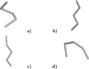
FIG. 4.: The four oligons with the highest proximity score for $l=5$.

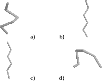
FIG. 5.: The four oligons with the highest proximity score for $l=6$.

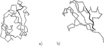
FIG. 6.: The best two representative for $l=5$ shown in their native protein environment.

FIG. 7.: When a subset of $m$ ranked oligons in used, not all arbitrary fragments of protein backbones can be represented within 0.65 Å. In this plot we show (solid lines) how much, on average it was necessary to distort the ten proteins in the test set so that each of their fragments fell within the proximity basin of the first $m$ ranked oligons. The dotted lines show the average deviations of the fitted and native $C_{\beta}$ positions computed for the test proteins.

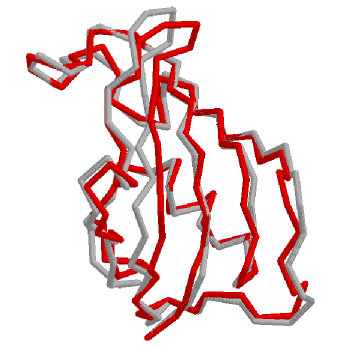
FIG. 8.: Illustration of the rigid fit procedure. The crystallographic structure of protein 1fkb (dark backbone) has been fitted by using the limited set of the first 40 oligons of length 5 (lighter backbone).

FIG. 9.: Number of emerging sequences (in natural-logarithmic scale) as a function of the considered fragments.

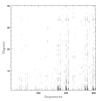
FIG. 10.: Two dimensional representation of the score matrix. In the x-axis the 614 sequences are labelled according to a conventional order. In the y-axis the best 40 oligons of length 5 are labelled according to their proximity score. The intensity of the colour is related to the values of the entries: the blank areas denote entries in the range 0-2, grey for the range 3-25, black for entries greater than 25.

FIG. 11.: Histograms showing the relative frequency with which four sequences occupy ranked oligons. The oligons are ranked according to their proximity score.

FIG. 12.: Histograms showing the relative frequency with which the first four oligons (ranked according to their proximity score) house different sequences. For this plot the same sequence-indexing of Fig. 10 is used

FIG. 13.: Monte-Carlo moves: (top) a single bead is moved; (middle) a set of amino-acids is moved by rotating a portion of the protein around a fixed axis; (bottom) a set of amino-acids is moved by pivotting part of the protein around a fixed point.

REFERENCES

- [1] Anfinsen, C. Principles that govern the folding of protein chains. Science 181:223-230, 1973.
- [2] Levinthal, C. How to fold graciously. Proceedings of a meeting held at Allerton House, Monticello, Illinois DeBrunner, Tsibris, Munck Eds, University of Illinois Press, 22-24, 1969.
- [3] Bryngelson, J. , Onuchic, J.N., Socci, J.N., & Wolynes, P.G. Funnels, patwhways and the energy landscape of protein folding: A Synthesis. Proteins: Struct. Funct. and Gen. 21:167-195, 1995.
- [4] Onuchic, J. N. Wolynes, P. G., Luthey-Schulten Z. and Socci, N. D. Toward an outline of the topography of a realistic protein: folding funnel. Proc. Natl. Acad. Sci. USA 92:3626-3630, 1995.
- [5] Karplus, M., Weaver, D.L. Protein folding dynamics. Nature 260:404-406, 1976.
- [6] Karplus, M., Weaver, D.L. Protein folding dynamics - the diffusion-collision model and experimental data. Protein Science 285:650-688, 1994.
- [7] Ptitsyin, O.B. Protein Folding: General physical model. FEBS Lett. 131:197-202, 1991.
- [8] Micheletti, C., Banavar, J.R., Maritan, A. & Seno., F. Protein Structures and Optimal Folding from a Geometrical Variational Principle. Phys. Rev. Lett. 82: 3372-3375, 1999.
- [9] Ramachandran, G.N. & Sasisekharan, V. Conformation of polypeptides and proteins. Adv. Prot. Chem. 23:283-437, 1968.
- [10] Covell, D.G. & Jernigan, R.L. Conformations of folded proteins in restricted spaces. Biochemistry 29:3287-3294, 1990.
- [11] Park, B.H. & Levitt, M. The complexity and accuracy of discrete state models. J. Mol. Biol. 249:493-507, 1995.
- [12] Park, B.H. & Levitt, M. Energy functions that discriminate X-ray and near native folds from well-constructed decoys. Journal of Molecular Biology 258:367-392, 1996.
- [13] Alwyn Jones, T. & Thirup, S. Using known substructures in protein model building and crystallography. The EMBO Journal 5: 819-822, 1986.
- [14] Unger, R., Harel, D., Wherland, S. & Sussman, J.L., A 3D building blocks approach to analyzing and predicting structure of proteins. Proteins: Structure, Function and Genetics 5: 355-373, 1989.
- [15] Rooman, M.J., Rodriguez, J. & Wodak, S.J. Automatic definition of recurrent local structure motifs in proteins. J. Mol. Biol. 213:327-336, 1990.
- [16] Rooman, M.J., Rodriguez, J. & Wodak, S.J. Automatic definition of recurrent local structure motifs in proteins. J. Mol. Biol. 213:337-350, 1990.
- [17] Pabo, C. Designing proteins and peptides. Nature 301:200, 1983.
- [18] Quinn, T.P., Tweedy, N.B. , Williams, R.W., Richardson, J.S. and Richardson, D.C. De-novo design, synthesis and characterization of a beta sandwich protein. Proc. Natl. Acad. Sci USA 91:8747-8751, 1994.
- [19] Johnson, M.S. , Srinivasan, N., Sowdhamini, R. & Blundell, T.L. Knowledge based protein modelling. Crit. Rev. in Biol. and Mol. Biol. 29:1-68, 1994.
- [20] MacQueen, J. 1967, Some methods for classification and analysis of multivariate observations”, proceedings of the Fifth Berkeley Symp. Math. Stat. Prob. I, 281-297, 1967
- [21] Fechteler, T., Dengler, U. & Schomburg, D. Prediction of protein 3-dimensional structures in insertion and deletion regions - a procedure for searching data-bases of representative protein fragments using geometric scoring criteria. J. Mol. Biol. 253:114-131, 1995.
- [22] Dahiyat, B.I. & Mayo, S.L. De novo protein design: Fully automated sequence selection. Science 278:82-87, 1997.
- [23] Micheletti, C., Seno, F., Maritan, A. & Banavar, J.R. Protein design in a lattice model of Hydrophobic and polar amino acids, Phys. Rev. Lett. 80:2237-2240, 1998.
- [24] Micheletti, C., Seno, F., Maritan, A. & Banavar, J.R. Design of proteins with hydrophobic and polar amino acids. Proteins: Struct. Funct. and Gen.: 32:80-87, 1998.
- [25] Micheletti, C., Seno, F., Maritan, A. & Banavar, J.R. Strategies for protein folding and design. Annals of Combinatorics 3:439-458, 1999.
- [26] Seno, F., Vendruscolo, M. , Maritan,A. & Seno,F. Optimal protein design procedure. Phys. Rev. Lett. 77:1901-1904, 1996.
- [27] Street, A.G. & Mayo, L.S. Computational protein design. Structure with folding and design 7:R105-109, 1999.
- [28] Miyazawa, S. & Jernigan, R.L. Estimation of Effective Interresidue Contact Energies from Protein Crystal Structures: Quasi-Chemical Approximation. Macromolecules 18:534-552, 1985.
- [29] Miyazawa, S. & Jernigan, R.L. Residue-Residue Potentials with a Favorable Contact Pair Term and an Unfavorable High Packing Density Term, for Simulation and Threading. Journal Molecular Biology 256:623-644, 1996.
- [30] Sippl, M.J. Calculation of conformational ensembles from potentials of mean force: an approach to the knowledge based prediction of local structures in globular proteins. J. Mol. Biol., 213:859-883, 1990.
- [31] Sippl, M.J. Knowledge based potentials for proteins. Current Opinion in Structural Biology 5 229-235, 1995 and references therein.
- [32] Crippen, G.M. Prediction of protein folding from amino acid sequence over discrete conformation space. Biochemistry 30:4232-4237, 1991.
- [33] Smithbrown, M.J., Kominos, D. & Levy, R.M. Global folding of proteins using a limited number of distance constraints. Protein Emgineering 6:605-614, 1993.
- [34] Seno, F. , Maritan, A. & Banavar, J.R. Interaction Potentials for Protein Folding. Protein: Struct. , Funct. and Gen 30:244-248, 1998.
- [35] Seno, F., Micheletti, C., Maritan, A. & Banavar, J.R. Variational approach to protein design and extraction of interaction potentials. Phys. Rev. Lett. 81:2172-2175, 1998.
- [36] Du, R., Grosberg, A.Y., & Tanaka, T. Models of protein interactions: how to choose one. em Fold. & Des. 3:203-211, 1998.
- [37] Settanni, G., Dima, R., Micheletti, C., Maritan, A., & Banavar, J.R. Determination of optimal effective interactions between amino acids in globular proteins, SISSA preprint.
- [38] Bastolla, U., Vendruscolo, M., and Knapp, E-W. Proc. Natnl. Acad. Sci. Usa, 97, 3977-3981 (2000).
- [39] Lesk, A.M., & Cothia, C. The response of protein structures to amino-acid sequence changes. Phil. Trans. R. Soc. Lond. A 317:345-356, 1986.
- [40] Prestrelsky, S.J., Williams, A.L. & Liebman, M.N. Generation of a substructure library for the description and classification of protein secondary structures. 1 Overview of the methods and results. Proteins: Struct. Funct. and Gen.: 21:430-439, 1992.
- [41] Hobohm, U., Scharf, M., Schneider, R. & Sander, C. Selection of representative protein data sets. Protein Science 1:409-417, 1992.
- [42] Sun, H.M. poster presented at the “Monte Carlo Workshop” - Florida State University - May 1999.
- [43] Aurora, R. Srinivanas, R. & Rose, G. D. Rules for alpha-helix termination by glycine. Science 264: 1126-1130, 1994.
- [44] Sibbald, P.R. Deducing protein structures using programming - exploiting minimum data of diverse types. Journ of Theor. Biol. 173:361-375, 1995.
- [45] Conklin, D. Machine discovery of protein motifs. Machine learning 21:125-150, 1995.
- [46] Lessel, U. & Schomburg, D. Creation and characterization of a new, non redundant fragment data bank. Protein Engineering 10:659-664, 1997.
- [47] Lacey, C. & Cole, S. Merger rates in hierarchical models of galaxy formation. Mon. Not. R. Astron. Soc. 262:627-649, 1993.
- [48] Kabsch, W. A discussion of the solution for the best rotation to relate two sets of vectors. Acta Crystallogr. A34:828-829, 1978.
- [49] Remington, S.J., & Matthews, B.W. A systematic approach to the comparison of protein structures. J. Mol. Biol. 140:77-99, 1980.
- [50] Wintjen, R.T., Rooman, M.J. & Wodak, S.J. Automatic classification and analysis of alpha alpha-turn motifs in protein. J. Mol. Biol. 255:235-353, 1996.
- [51] Pauling, L., Corey, R. B. & Branson, H. R. The structure of proteins: two hydrogen- bonded helical configurations of the polypeptide chain. Proc. Nat. Acad. Sci. 37:205-211, 1951.
- [52] Socci, N. D., Bialek, W. S. & Onuchic, J. N. Properties and origins of protein secondary structures. Phys. Rev. E 49:3440-3443, 1994.
- [53] Aurora, R., Creamer, T. P., Srinivasan, R. & Rose, G. D., Local interactions in protein folding: Lessons from the alpha-helix. J. Biol. Chem. 272, 1413-1416, 1997
- [54] Hunt, N. G., Gregoret, L. M. & Cohen, F. E. The origins of protein secondary structure - effects of packing density and hydrogen-bonding studied by a fast conformational search. J. Mol. Biol. 241:214-225, 1994.
- [55] Maritan, A., Micheletti, C. & Banavar, J.R. Role of Secondary Motifs in Fast Folding Polymers: A Dynamical Variational Principle, Phys. Rev. Lett, 84, 3009, (2000)
- [56] Go, N. & Scheraga, H.A. On the use of classical mechanics in treatment of polymer chain conformations. Macromolecules 9:535-542, 1976.
- [57] Micheletti, C., Maritan, A. & Seno, F. In preparation.
- [58] Brandsen, C. & Tooze, J. in Introduction to protein structure, Garland Publishing, New York, 1991.
- [59] Creighton, T.E. in Proteins: structures and molecular properties, W. H. Freeman ed., New York, 1992.
- [60] Srinivasan, R. and Rose, G. D. A physical basis for protein secondary structure. Proc. Natnl. Acad. Sci. USA 96: 14258-14263, 1999.
- [61] Altschul, S.F. Amino acid substitution matrices from an information theoretic perspective. J. Mol. Biol. 219:555-565, 1991.
- [62] Huang, E.S., Koehl,P., Levitt, M. Pappu, R.V. & Ponder, J.W. Accuracy of side-chain prediction upon near-native protein backbones generated by ab initio folding methods. Proteins: Struct. Funct. and Gen. 33:204-207, 1998.
- [63] Chan, H. S. Folding alphabets, Nature Struct. Biol., 6:994-996, (1999)
- [64] Bystroff, C. & Baker, D. Prediction of local structure in proteins using a library of sequence-structure motifs. J. Mol. Biol. 281:565-577, 1998.
- [65] Han, K.F. & Baker, D. Global properties of the mapping between local amino acid sequence and local structure in proteins, Proc. Natl. Acad, Sci, USA 93:5814-5818, 1996.
- [66] Gerroff, I., Milchev, A. , Binder, K. & Paul, W. A new off-lattice monte carlo model for polymers - A comparison of static and dynamic properties with the bond fluctuation model and application to random media. J. Chem. Phys. 98:6256-6539, 1993.
- [67] Sokal, A.D. Monte Carlo methods for the self-avoiding walk. Nuclear Physics B47 172-179, 1996.
- [68] Skolnick, J. & Kolinski, A. Monte Carlo approaches to the protein folding problem. Adv. in Chem. Phys. 105:203-242, 1999.