Quantum Phase Transitions

Abstract

Phase transitions which occur at zero temperature when some non-thermal parameter like pressure, chemical composition or magnetic field is changed are called quantum phase transitions. They are caused by quantum fluctuations which are a consequence of Heisenberg’s uncertainty principle. These lecture notes give a pedagogical introduction to quantum phase transitions. After collecting a few basic facts about phase transitions and critical behavior we discuss the importance of quantum mechanics and the relation between quantum and classical transitions as well as their experimental relevance. As a primary example we then consider the Ising model in a transverse field. We also briefly discuss quantum phase transitions in itinerant electron systems and their connection to non-Fermi liquid behavior.

1 Introduction: From the melting of ice to quantum criticality

When a piece of ice is taken out of the freezer, in the beginning its properties change only slowly with increasing temperature. At $0^{\circ}$C, however, a drastic change happens. The thermal motion of the water molecules becomes so strong that it destroys the crystal structure. The ice melts, and a new phase of water forms, the liquid phase. This process is an example for a phase transition. At the transition temperature of $0^{\circ}$C the solid and the liquid phases of water coexist. A finite amount of heat, the so-called latent heat, is necessary to transform the ice into liquid water. Phase transitions which involve latent heat are usually called first-order transitions.

Another well known example of a phase transition is the magnetic transition of iron. At room temperature iron is ferromagnetic, i.e. it possesses a spontaneous magnetization. With increasing temperature the magnetization decreases continuously. It vanishes at the Curie temperature of $770^{\circ}$C, and above this temperature iron is paramagnetic. This is a phase transition from a ferro- to a paramagnet. In contrast to the previous example there is no phase coexistence at the transition temperature, the two phases rather become indistinguishable. Consequently, there is no latent heat. This type of phase transitions are called continuous transitions or second-order transitions. They are the result of a competition between order and thermal fluctuations. When approaching the transition point the typical length and time scales of the fluctuations diverge, leading to singularities in many physical quantities. The diverging correlation length at a continuous phase transition was first observed in 1869 in a famous experiment by Andrews Andrews1869 . He discovered that the properties of the liquid and the vapor phases of carbon dioxide became indistinguishable at a temperature of about 31 ^∘C and 73 atmospheres pressure. In the vicinity of this point the carbon dioxide became opaque, i.e. it strongly scattered visible light, indicating that the length scale of the density fluctuations had reached the wave length of the light. Andrews called this special point in the phase diagram the critical point and the strong light scattering in its vicinity the critical opalescence.

More formally one can define a phase transition as the occurrence of a singularity in the thermodynamic quantities as functions of the external parameters. Phase transitions have played, and continue to play, an essential role in shaping our world. The large scale structure of the universe is the result of a sequence of phase transitions during the very early stages of its development. Even our everyday life is unimaginable without the never ending transformations of water between ice, liquid and vapor. Understanding the properties of phase transitions and in particular those of critical points has been a great challenge for theoretical physics. More than a century has gone by from the first discoveries until a consistent picture emerged. However, the theoretical concepts established during this development, viz., scaling and the renormalization group Wilson71 , now belong to the central paradigms of modern physics.

In the last decade considerable attention has concentrated on a class of phase transitions which are qualitatively very different from the examples discussed above. These new transitions occur at zero temperature when a non-thermal parameter like pressure, chemical composition or magnetic field is changed. The fluctuations which destroy the long-range order in these transitions cannot be of thermal nature since thermal fluctuations do not exist at zero temperature. Instead, they are quantum fluctuations which are a consequence of Heisenberg’s uncertainty principle. For this reason phase transitions at zero temperature are called quantum phase transitions, in contrast to thermal or classical phase transitions at finite temperatures. (The justification for calling all thermal phase transitions classical will become clear in Sec. 3)

As an illustration of classical and quantum phase transitions we show the magnetic phase diagram of the transition metal compound MnSi in Fig. 1.

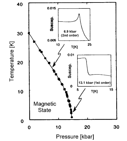
Figure 1: Magnetic phase diagram of MnSi (after Ref. PML95 ). The peculiar behavior of the magnetic susceptibility shown in the insets is a consequence of the interplay between the magnetic and other fermionic degrees of freedom us_fm ).

At ambient pressure MnSi is a paramagnetic metal for temperatures larger than $T_{c}=30$ K. Below $T_{c}$ it orders ferromagnetically but remains metallic. This transition is a thermal continuous phase transition analogous to that in iron discussed above. Applying pressure reduces the transition temperature, and at about 14 kBar the magnetic phase vanishes. Thus, at 14 kBar MnSi undergoes a quantum phase transition from a ferro- to a paramagnet. While this is a very obvious quantum phase transition, its properties are rather complex due to the interplay between the magnetic degrees of freedom and other fermionic excitations (for details see us_fm ).

At a first glance quantum phase transitions seem to be a purely academic problem since they occur at isolated parameter values and at zero temperature which is inaccessible in an experiment. However, within the last decade it has turned out that the opposite is true. Quantum phase transitions do have important, experimentally relevant consequences, and they are believed to provide keys to many new and exciting phenomena in condensed matter physics, such as the quantum Hall effects, the localization problem, non-Fermi liquid behavior in metals or high-$T_{c}$ superconductivity.

These lecture notes are intended as a pedagogical introduction to quantum phase transitions. In section 2 we first collect a few basic facts about phase transitions and critical behavior. In section 3 we then investigate the importance of quantum mechanics for the physics of phase transitions and the relation between quantum and classical transitions. Section 4 is devoted to a detailed analysis of the physics in the vicinity of a quantum critical point. We then discuss two examples: In section 5 we consider one of the paradigmatic models in this field, the Ising model in a transverse field, and in section 6 we briefly discuss quantum phase transitions in itinerant electron systems and their connection to non-Fermi liquid behavior.

Those readers who want to learn more details about quantum phase transitions and the methods used to study them, should consult one of the recent review articles, e.g. Refs. sgcs97 ; kb97 ; vojta2000 , or the excellent text book on quantum phase transitions by Sachdev sachdev00 .

2 Basic concepts of phase transitions and critical behavior

In this section we briefly collect the basic concepts of continuous phase transitions and critical behavior which are necessary for the later discussions. For a detailed exposure the reader is referred to one of the text books on this subject, e.g., those by Ma Ma76 or Goldenfeld Goldenfeld92 ).

A continuous phase transition can usually be characterized by an order parameter, a concept first introduced by Landau Landau37 . An order parameter is a thermodynamic quantity that is zero in one phase (the disordered) and non-zero and non-unique in the other (the ordered) phase. Very often the choice of an order parameter for a particular transition is obvious as, e.g., for the ferromagnetic transition where the total magnetization is an order parameter. Sometimes, however, finding an appropriate order parameter is a complicated problem by itself, e.g., for the disorder-driven localization-delocalization transition of non-interacting electrons.

While the thermodynamic average of the order parameter is zero in the disordered phase, its fluctuations are non-zero. If the phase transition point, i.e., the critical point, is approached the spatial correlations of the order parameter fluctuations become long-ranged. Close to the critical point their typical length scale, the correlation length $\xi$, diverges as

$$\xi\propto|t|^{-\nu}$$ (1)

where $\nu$ is the correlation length critical exponent and $t$ is some dimensionless measure of the distance from the critical point. If the transition occurs at a non-zero temperature $T_{c}$, it can be defined as $t=|T-T_{c}|/T_{c}$. The divergence of the correlation length when approaching the transition is illustrated in Fig. 2 which shows computer simulation results for the phase transition in a two-dimensional Ising model.

Figure 2: Snapshots of the spin configuration of a two-dimensional Ising model at different temperatures (a black dot corresponds to spin up, an empty site means spin down). From left to right: $T=2T_{c}$, $T=1.3T_{c}$, $T=T_{c}$. The correlation length increases with decreasing temperature and diverges at $T=T_{c}$. Here the system fluctuates at all length scales.

In addition to the long-range correlations in space there are analogous long-range correlations of the order parameter fluctuations in time. The typical time scale for a decay of the fluctuations is the correlation (or equilibration) time $\tau_{c}$. As the critical point is approached the correlation time diverges as

$$\tau_{c}\propto\xi^{z}\propto|t|^{-\nu z}$$ (2)

where $z$ is the dynamical critical exponent. Close to the critical point there is no characteristic length scale other than $\xi$ and no characteristic time scale other than $\tau_{c}$. As already noted by Kadanoff Kadanoff66 , this is the physics behind Widom’s scaling hypothesis Widom65 , which we will now discuss.

Let us consider a classical system, characterized by its Hamiltonian

$$H(p_{i},q_{i})=H_{kin}(p_{i})+H_{pot}(q_{i})$$ (3)

where $q_{i}$ and $p_{i}$ are the generalized coordinates and momenta, and $H_{kin}$ and $H_{pot}$ are the kinetic and potential energies, respectively. In such a system statics and dynamics decouple, i.e., the momentum and position sums in the partition function

$$Z=\int\prod dp_{i}e^{-H_{kin}/k_{B}T}~{}\int\prod dq_{i}e^{-H_{pot}/k_{B}T}=Z_{kin}Z_{pot}$$ (4)

are completely independent from each other. The kinetic contribution to the free energy density $f=-(k_{B}T/V)\log Z$ will usually not display any singularities, since it derives from the product of simple Gaussian integrals. Therefore one can study phase transitions and the critical behavior using effective time-independent theories like the classical Landau-Ginzburg-Wilson theory. In this type of theories the free energy is expressed as a functional of the order parameter $M({\bf r})$, which is time-independent but fluctuates in space. All other degrees of freedom have been integrated out in the derivation of the theory starting from a microscopic Hamiltonian. In its simplest form Wilson71 ; Landau37 ; Ginzburg60 valid, e.g., for an Ising ferromagnet, the Landau-Ginzburg-Wilson functional $\Phi[M]$ reads

$$\Phi[M] = \int d^{d}r~{}M({\bf r})\left(-\frac{\partial^{2}}{\partial{\bf r}^{2}}+t\right)M({\bf r})+u\int d^{d}r~{}M^{4}({\bf r})-B\int d^{d}r~{}M({\bf r}),$$ (5)

$$Z = \int D[M]e^{-\Phi[M]}\quad,$$ (6)

where $B$ is the field conjugate to the order parameter (the magnetic field in case of a ferromagnet).

Since close to the critical point the correlation length is the only relevant length scale, the physical properties must be unchanged, if we rescale all lengths in the system by a common factor $b$, and at the same time adjust the external parameters in such a way that the correlation length retains its old value. This observation gives rise to the homogeneity relation for the free energy density,

$$f(t,B)=b^{-d}f(t\,b^{1/\nu},B\,b^{y_{B}}).$$ (7)

Here $y_{B}$ is another critical exponent and $d$ is the space dimensionality. The scale factor $b$ is an arbitrary positive number. Analogous homogeneity relations for other thermodynamic quantities can be obtained by differentiating the free energy. The homogeneity law (7) was first obtained phenomenologically by Widom Widom65 . Within the framework of the renormalization group theory Wilson71 it can be derived from first principles.

In addition to the critical exponents $\nu,~{}y_{B}$ and $z$ defined above, a number of other exponents is in common use. They describe the dependence of the order parameter and its correlations on the distance from the critical point and on the field conjugate to the order parameter. The definitions of the most commonly used critical exponents are summarized in Table 1.

Table 1: Definitions of the commonly used critical exponents in the ‘magnetic language’, i.e., the order parameter is the magnetization $m=\langle M\rangle$, and the conjugate field is a magnetic field $B$. $t$ denotes the distance from the critical point and $d$ is the space dimensionality. (The exponent $y_{B}$ defined in (7) is related to $\delta$ by $y_{B}=d\,\delta/(1+\delta)$.)

	exponent	definition	conditions
specific heat	$\alpha$	$c\propto|t|^{-\alpha}$	$t\to 0,B=0$
order parameter	$\beta$	$m\propto(-t)^{\beta}$	$t\to 0$ from below, $B=0$
susceptibility	$\gamma$	$\chi\propto|t|^{-\gamma}$	$t\to 0,B=0$
critical isotherm	$\delta$	$B\propto|m|^{\delta}{\rm sign}(m)$	$B\to 0,t=0$
correlation length	$\nu$	$\xi\propto|t|^{-\nu}$	$t\to 0,B=0$
correlation function	$\eta$	$G(r)\propto|r|^{-d+2-\eta}$	$t=0,B=0$
dynamical	$z$	$\tau_{c}\propto\xi^{z}$	$t\to 0,B=0$

Note that not all the exponents defined in Table 1 are independent from each other. The four thermodynamic exponents $\alpha,\beta,\gamma,\delta$ can all be obtained from the free energy (7) which contains only two independent exponents. They are therefore connected by the so-called scaling relations

$$2-\alpha=2\beta+\gamma~{},\qquad 2-\alpha=\beta(\delta+1)~{}.$$ (8)

Analogously, the exponents of the correlation length and correlation function are connected by two so-called hyperscaling relations

$$2-\alpha=d\,\nu~{},\qquad\gamma=(2-\eta)\nu~{}.$$ (9)

Since statics and dynamics decouple in classical statistics the dynamical exponent $z$ is completely independent from all the others.

The set of critical exponents completely characterizes the critical behavior at a particular phase transition. One of the most remarkable features of continuous phase transitions is universality, i.e., the fact that the critical exponents are the same for entire classes of phase transitions which may occur in very different physical systems. These classes, the so-called universality classes, are determined only by the symmetries of the Hamiltonian and the spatial dimensionality of the system. This implies that the critical exponents of a phase transition occurring in nature can be determined exactly (at least in principle) by investigating any simplistic model system belonging to the same universality class, a fact that makes the field very attractive for theoretical physicists. The mechanism behind universality is again the divergence of the correlation length. Close to the critical point the system effectively averages over large volumes rendering the microscopic details of the Hamiltonian unimportant.

The critical behavior at a particular transition is crucially determined by the relevance or irrelevance of order parameter fluctuations. It turns out that fluctuations become increasingly important if the spatial dimensionality of the system is reduced. Above a certain dimension, called the upper critical dimension $d_{c}^{+}$, fluctuations are irrelevant, and the critical behavior is identical to that predicted by mean-field theory (for systems with short-range interactions and a scalar or vector order parameter $d_{c}^{+}=4$). Between $d_{c}^{+}$ and a second special dimension, called the lower critical dimension $d_{c}^{-}$, a phase transition still exists but the critical behavior is different from mean-field theory. Below $d_{c}^{-}$ fluctuations become so strong that they completely suppress the ordered phase.

3 How important is quantum mechanics?

The question of to what extent quantum mechanics is important for understanding a continuous phase transition is a multi-layered question. One may ask, e.g., whether quantum mechanics is necessary to explain the existence and the properties of the ordered phase. This question can only be decided on a case-by-case basis, and very often quantum mechanics is essential as, e.g., for superconductors. A different question to ask would be how important quantum mechanics is for the asymptotic behavior close to the critical point and thus for the determination of the universality class the transition belongs to.

It turns out that the latter question has a remarkably clear and simple answer: Quantum mechanics does not play any role for the critical behavior if the transition occurs at a finite temperature. It does play a role, however, at zero temperature. In the following we will first give a simple argument explaining these facts. To do so it is useful to distinguish fluctuations with predominantly thermal and quantum character depending on whether their thermal energy $k_{B}T$ is larger or smaller than the quantum energy scale $\hbar\omega_{c}$. We have seen in the preceeding section that the typical time scale $\tau_{c}$ of the fluctuations diverges as a continuous transition is approached. Correspondingly, the typical frequency scale $\omega_{c}$ goes to zero and with it the typical energy scale

$$\hbar\omega_{c}\propto|t|^{\nu z}~{}.$$ (10)

Quantum fluctuations will be important as long as this typical energy scale is larger than the thermal energy $k_{B}T$. If the transition occurs at some finite temperature $T_{c}$ quantum mechanics will therefore become unimportant for $|t|<t_{x}$ with the crossover distance $t_{x}$ given by

$$t_{x}\propto T_{c}^{1/\nu z}~{}.$$ (11)

We thus find that the critical behavior asymptotically close to the transition is entirely classical if the transition temperature $T_{c}$ is nonzero. This justifies to call all finite-temperature phase transitions classical transitions, even if the properties of the ordered state are completely determined by quantum mechanics as is the case, e.g., for the superconducting phase transition of mercury at $T_{c}=4.2$ K. In these cases quantum fluctuations are obviously important on microscopic scales, while classical thermal fluctuations dominate on the macroscopic scales that control the critical behavior. This also implies that only universal quantities like the critical exponents will be independent of quantum mechanics while non-universal quantities like the critical temperature in general will depend on quantum mechanics.

If, however, the transition occurs at zero temperature as a function of a non-thermal parameter like the pressure $p$, the crossover distance $t_{x}$ equals zero since there are no thermal fluctuations. (Note that at zero temperature the distance $t$ from the critical point cannot be defined via the reduced temperature. Instead, one can define $t=|p-p_{c}|/p_{c}$.) Thus, at zero temperature the condition $|t|<t_{x}$ is never fulfilled, and quantum mechanics will be important for the critical behavior. Consequently, transitions at zero temperature are called quantum phase transitions.

Let us now generalize the homogeneity law (7) to the case of a quantum phase transition. We consider a system characterized by a Hamiltonian $H$. In a quantum problem kinetic and potential part of $H$ in general do not commute. In contrast to the classical partition function (4) the quantum mechanical partition function does not factorize, i.e., statics and dynamics are always coupled. The canonical density operator $e^{-H/k_{B}T}$ looks exactly like a time evolution operator in imaginary time $\tau$ if one identifies

$$1/k_{B}T=\tau=-i\Theta/\hbar$$ (12)

where $\Theta$ denotes the real time. This naturally leads to the introduction of an imaginary time direction into the system. An order parameter field theory analogous to the classical Landau-Ginzburg-Wilson theory (6) therefore needs to be formulated in terms of space and time dependent fields. The simplest example of a quantum Landau-Ginzburg-Wilson functional, valid for, e.g., an Ising model in a transverse field (see section 5), reads

$$\Phi[M] = \int_{0}^{1/k_{B}T}d\tau\int d^{d}r~{}M({\bf r},\tau)\left(-\frac{\partial^{2}}{\partial{\bf r}^{2}}-\frac{\partial^{2}}{\partial\tau^{2}}+t\right)M({\bf r},\tau)~{}+$$ (13)

$$+ u\int_{0}^{1/k_{B}T}d\tau\int d^{d}r~{}M^{4}({\bf r},\tau)~{}-~{}B\int_{0}^{1/k_{B}T}d\tau\int d^{d}r~{}M({\bf r},\tau)~{}.$$ (14)

Let us note that the coupling of statics and dynamics in quantum statistical mechanics also leads to the fact that the universality classes for quantum phase transitions are smaller than those for classical transitions. Systems which belong to the same classical universality class may display different quantum critical behavior, if their dynamics differ.

The classical homogeneity law (7) for the free energy density can now easily be adopted to the case of a quantum phase transition. At zero temperature the imaginary time acts similarly to an additional spatial dimension since the extension of the system in this direction is infinite. According to (2), time scales like the $z$th power of a length. (In the simple example (14) space and time enter the theory symmetrically leading to $z=1$.) Therefore, the homogeneity law for the free energy density at zero temperature reads

$$f(t,B)=b^{-(d+z)}f(t\,b^{1/\nu},B\,b^{y_{B}})~{}.$$ (15)

Comparing this relation to the classical homogeneity law (7) directly shows that a quantum phase transition in $d$ spatial dimensions is equivalent to a classical transition in $d+z$ spatial dimensions. Thus, for a quantum phase transition the upper critical dimension, above which mean-field critical behavior becomes exact, is reduced by $z$ compared to the corresponding classical transition. Note, however, that the mapping of a quantum phase transition to the equivalent classical transition in general leads to unusual anisotropic classical systems. Furthermore, the mapping is valid for the thermodynamics only. Other properties like the real time dynamics at finite temperatures require more careful considerations (see, e.g., Ref. sachdev00 ).

Now the attentive reader may again ask: Why are quantum phase transitions more than an academic problem? Any experiment is done at a non-zero temperature where, as we have explained above, the asymptotic critical behavior is classical. The answer is provided by the crossover condition (11): If the transition temperature $T_{c}$ is very small quantum fluctuations will remain important down to very small $t$, i.e., very close to the phase boundary. At a more technical level, the behavior at small but non-zero temperatures is determined by the crossover between two types of critical behavior, viz. quantum critical behavior at $T=0$ and classical critical behavior at non-zero temperatures. Since the ‘extension of the system in imaginary time direction’ is given by the inverse temperature $1/k_{B}T$ the corresponding crossover scaling is equivalent to finite size scaling in imaginary time direction. The crossover from quantum to classical behavior will occur when the correlation time $\tau_{c}$ reaches $1/k_{B}T$ which is equivalent to the condition (11). By adding the temperature as an explicit parameter and taking into account that in imaginary-time formalism it scales like an inverse time (12), we can generalize the quantum homogeneity law (15) to finite temperatures,

$$f(t,B,T)=b^{-(d+z)}f(t\,b^{1/\nu},B\,b^{y_{B}},T\,b^{z})~{}.$$ (16)

Once the critical exponents $z$, $\nu$, and $y_{B}$ and the scaling function $f$ are known this relation completely determines the thermodynamic properties close to the quantum phase transition.

4 Quantum-critical points

We now use the general scaling picture developed in the last section to discuss the physics in the vicinity of the quantum critical point. There are two qualitatively different types of phase diagrams depending on the existence or non-existence of long-range order at finite temperatures. These phase diagrams are schematically shown in Fig. 3.

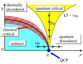
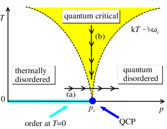
Figure 3: Schematic phase diagrams in the vicinity of a quantum critical point (QCP) for situations where an ordered phase exists at finite temperatures (left) and situations where order exists at zero temperature only (right). The solid line marks the boundary between ordered and disordered phase. The different regions and paths (a) and (b) are discussed in the text.

Here $p$ stands for the (non-thermal) parameter which tunes the quantum phase transition. In addition to the phase boundary the phase diagrams show a number of crossover lines where the properties of the system change smoothly. They separate regions with different characters of the fluctuations.

The first type of phase diagrams describes situations where an ordered phase exists at finite temperatures. As discussed in the last section classical fluctuations will dominate in the vicinity of the phase boundary (in the hatched region in Fig. 3). According to (11) this region becomes narrower with decreasing temperature. An experiment performed along path (a) will therefore observe a crossover from quantum critical behavior away from the transition to classical critical behavior asymptotically close to it. At very low temperatures the classical region may become so narrow that it is actually unobservable in an experiment. In the quantum disordered region ($p>p_{c}$, small $T$) the physics is dominated by quantum fluctuations, the system essentially looks as in its quantum disordered ground state at $p>p_{c}$. In contrast, in the thermally disordered region the long-range order is destroyed mainly by thermal fluctuations.

Between the quantum disordered and the thermally disordered regions is the so-called quantum critical region CHN89 , where both types of fluctuations are important. It is located at the critical $p$ but, somewhat counter-intuitively, at comparatively high temperatures. Its boundaries are also determined by (11) but in general with a prefactor different from that of the asymptotic classical region. The physics in the quantum critical region is controlled by the quantum critical point: The system ’looks critical’ with respect to $p$ (due to quantum fluctuations) but is driven away from criticality by thermal fluctuations (i.e., the critical singularities are exclusively protected by the temperature $T$). In an experiment carried out along path (b) the physics will therefore be dominated by the critical fluctuations which diverge according to the temperature scaling at the quantum critical point.

The second type of phase diagram occurs if an ordered phase exists at zero temperature only (as is the case for two-dimensional quantum antiferromagnets). In this case there will be no true phase transition in any experiment. However, an experiment along path (a) will show a very sharp crossover which becomes more pronounced with decreasing temperature. Furthermore, the system will display quantum critical behavior in the above-mentioned quantum critical region close to the critical $p$ and at higher temperatures.

5 Example: Transverse field Ising model

In this section we want to illustrate the general ideas presented in sections 3 and 4 by discussing a paradigmatic example, viz. the Ising model in a transverse field. An experimental realization of this model can be found in the low-temperature magnetic properties of LiHoF₄. This material is an ionic crystal, and at sufficiently low temperatures the only magnetic degrees of freedom are the spins of the Holmium atoms. They have an easy axis, i.e. they prefer to point up or down with respect to a certain crystal axis. Therefore they can be represented by Ising spin variables. Spins at different Holmium atoms interact via a magnetic dipole-dipole interaction. Without external magnetic field the ground state is a fully polarized ferromagnet.

In 1996 Bitko, Rosenbaum and Aeppli BRA96 measured the magnetic properties of LiHoF₄ as a function of temperature and a magnetic field which was applied perpendicular to the preferred spin orientation. The resulting phase diagram is shown in Fig. 4.

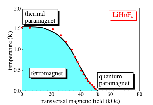
Figure 4: Magnetic phase diagram of LiHoF₄ (after BRA96 ).

In order to understand this phase diagram we now consider a minimal microscopic model for the relevant magnetic degrees of freedom in LiHoF₄, the Ising model in a transverse field. Choosing the $z$-axis to be the Ising axis its Hamiltonian is given by

$$H=-J\sum_{\langle ij\rangle}S_{i}^{z}\,S_{j}^{z}-h\sum_{i}S_{i}^{x}~{}.$$ (17)

Here $S_{i}^{z}$ and $S_{i}^{x}$ are the $z$ and $x$ components of the Holmium spin at lattice site $i$, respectively. The first term in the Hamiltonian describes the ferromagnetic interaction between the spins which we restrict to nearest neighbors for simplicity. The second term is the transversal magnetic field. For zero field $h=0$, the model reduces to the well-known classical Ising model. At zero temperature all spins are parallel. At a small but finite temperature a few spins will flip into the opposite direction. With increasing temperature the number and size of the flipped regions increases, reducing the total magnetization. At the critical temperature (about 1.5 K for LiHoF₄) the magnetization vanishes, and the system becomes paramagnetic. The resulting transition is a continuous classical phase transition caused by thermal fluctuations.

Let us now consider the influence of the transverse magnetic field. To do so, it is convenient to rewrite the field term as

$$-h\sum_{i}S_{i}^{x}=-h\sum_{i}(S_{i}^{+}+S_{i}^{-})$$ (18)

where $S_{i}^{+}$ and $S_{i}^{-}$ are the spin flip operators at site $i$. From this representation it is easy to see that the transverse field will cause spin flips. These flips are the quantum fluctuations discussed in the preceeding sections. If the transverse field becomes larger than some critical field $h_{c}$ (about 50 kOe in LiHoF₄) they will destroy the ferromagnetic long-range order in the system even at zero temperature. This transition is a quantum phase transition driven exclusively by quantum fluctuations.

For the transversal field Ising model the quantum-to-classical mapping discussed in section 3 can be easily demonstrated at a microscopic level. Consider a one-dimensional classical Ising chain with the Hamiltonian

$$H_{cl}=-J\sum_{i=1}^{N}S_{i}^{z}\,S_{i+1}^{z}~{}.$$ (19)

Its partition function is given by

$$Z={\rm Tr}\,e^{-H_{cl}/T}={\rm Tr}\,e^{J\sum_{i=1}^{N}S_{i}^{z}S_{i+1}^{z}/T}={\rm Tr}\,\prod_{i=1}^{N}M_{i,i+1}~{},$$ (20)

where $\mathbf{M}$ is the so called transfer matrix. It can be represented as

$$\mathbf{M}=\left(\begin{array}[]{cc}e^{J/T}&e^{-J/T}\\ e^{-J/T}&e^{J/T}\end{array}\right)=e^{J/T}(1+e^{-2J/T}S^{x})\approx\exp(J/T+e^{-2J/T}S^{x})~{}.$$ (21)

Except for a multiplicative constant the partition function of the classical Ising chain has the same form as that of a single quantum spin in a transverse field, $H_{Q}=-h\,S^{x}$, which can be written as

$$Z={\rm Tr}e^{-H_{Q}/T_{Q}}={\rm Tr}e^{hS^{x}/T_{Q}}={\rm Tr}\prod_{i=1}^{N}e^{hS^{x}/(T_{Q}N)}~{}.$$ (22)

Thus, a single quantum spin can be mapped onto a classical Ising chain. This considerations can easily be generalized to a $d$-dimensional transversal field (quantum) Ising model which can be mapped onto a $(d+1)$-dimensional classical Ising model. Consequently, the dynamical exponent $z$ must be equal to unity for the quantum phase transitions of transverse field Ising models. Using a path integral approach analogous to Feynman’s treatment of a single quantum particle, the quantum Landau-Ginzburg-Wilson functional (14) can be derived from (22) or its higher-dimensional analogs.

6 Quantum phase transitions and non-Fermi liquids

In this section we want to discuss a particularly important consequence of quantum phase transitions, viz. non-Fermi liquid behavior in an itinerant electron system. In a normal metal the electrons form a Fermi liquid, a concept developed by Landau in the 1950s Landau56 . In this state the strongly (via Coulomb potential) interacting electrons essentially behave like almost non-interacting quasiparticles with renormalized parameters (like the effective mass). This permits very general and universal predictions for the low-temperature properties of metallic electrons: For sufficiently low temperatures the specific heat is supposed to be linear in the temperature, the magnetic susceptibility approaches a constant, and the electric resistivity has the form $\rho(T)=\rho_{0}+AT^{2}$ (where $\rho_{0}$ is the residual resistance caused by impurities).

The Fermi liquid concept is extremely successful, it describes the vast majority of conducting materials. However, in the last years there have been experimental observations that are in contradiction to the Fermi liquid picture, e.g. in the normal phase of the high-$T_{c}$ superconducting materials HighTc or in heavy fermion systems HeavyF . These are compounds of rare-earth elements or actinides where the quasiparticle effective mass is up to a few thousand times larger than the electron mass.

Fig. 5 shows an example for such an observation, viz. the specific heat coefficient $C/T$ of the heavy-fermion system von CeCu_6-xAu_x as a function of the temperature $T$.

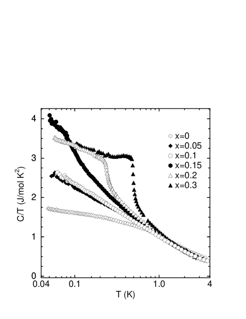
Figure 5: Specific heat coefficient $C/T$ of CeCu_6-xAu_x as a function of temperature $T$ for different gold concentration $x$ (after Lohn96 ).

In a Fermi liquid $C/T$ should become constant for sufficiently low temperatures. Instead, in Fig. 5 $C/T$ shows a pronounced temperature dependence. In particular, the sample with a gold concentration of $x=0.1$ shows a logarithmic temperature dependence, $C/T\sim\log(1/T)$, over a wide temperature range.

In order to understand these deviations from the Fermi liquid and in particular the qualitative differences between the behaviors at different $x$ it is helpful to relate the specific heat to the magnetic phase diagram of CeCu_6-xAu_x, which is shown in Fig. 6. Pure CeCu₆ is a paramagnet, but by alloying with gold it can become antiferromagnetic. The quantum phase transition is roughly at a critical gold concentration of $x_{c}=0.1$ (and $T=0$).

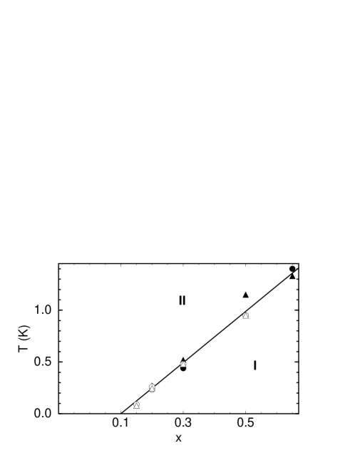
Figure 6: Magnetic phase diagram of CeCu_6-xAu_x (after Lohn96 ). I is the antiferromagnetic phase, II the paramagnetic phase.

Let us first discuss the specific heat at the critical concentration $x_{c}=0.1$. A comparison with the schematic phase diagram in Fig. 3 shows that at this concentration the entire experiment is done in the quantum critical region (path (b)). When approaching the quantum critical point, i.e. with decreasing temperature the antiferromagnetic fluctuations diverge. The electrons are scattered off these fluctuations which hinders their movement and therefore increases the effective mass of the quasiparticles. In the limit of zero temperature the effective mass diverges and with it the specific heat coefficient $C/T$.

In an experiment at a gold concentration slightly above or below the critical concentration the system will be in the quantum critical region at high temperatures. Here the specific heat agrees with that at the critical concentration. However, with decreasing temperature the system leaves the quantum-critical region, either towards the quantum disordered region (for $x<x_{c}$) or into the ordered phase (for $x>x_{c}$). In the first case there will be a crossover from the quantum critical behavior $C/T\sim\log(1/T)$ to conventional Fermi liquid behavior $C/T={\rm const}$. This can be seen for the $x=0$ data in Fig. 5. In the opposite case, $x>x_{c}$ the system undergoes an antiferromagnetic phase transition at some finite temperature, connected with a singularity in the specific heat. In Fig. 5 this singularity is manifest as a pronounced shoulder.

In conclusion, the non-Fermi liquid behavior of CeCu_6-xAu_x can be completely explained (at least qualitatively) by the antiferromagnetic quantum phase transition at the critical gold concentration of $x_{c}=0.1$. The deviations from the Fermi liquid occur in the quantum critical region where the electrons are scattered off the diverging magnetic fluctuations. Analogous considerations can be applied to other observables, e.g. the magnetic susceptibility or the electric resistivity.

7 Summary and Outlook

Quantum phase transitions are a fascinating subject in todays condensed matter physics. They open new ways of looking at complex situations and materials for which conventional methods like perturbation theory fail. So far, only the simplest, and the most obvious cases have been studied in detail which leaves a lot of interesting research for the future.

This work was supported in part by the DFG under grant Nos. Vo659/2 and SFB393/C2 and by the NSF under grant No. DMR–98–70597.

References

- (1) T. Andrews: Phil. Trans. R. Soc. 159, 575 (1869)
- (2) K. G. Wilson: Phys. Rev. B 4, 3174 (1971); ibid 3184
- (3) C. Pfleiderer, G. J. McMullan, and G. G. Lonzarich: Physica B 206&207, 847 (1995)
- (4) T. Vojta, D. Belitz, R. Narayanan, and T.R. Kirkpatrick: Z. Phys. B 103, 451 (1997); D. Belitz, T.R. Kirkpatrick and T. Vojta: Phys. Rev. Lett 82, 4707 (1999)
- (5) S.L. Sondhi, S.M. Girvin, J.P. Carini, and D. Shahar: Rev. Mod. Phys. 69, 315 (1997)
- (6) T.R. Kirkpatrick and D. Belitz:‘Quantum phase transitions in electronic systems’. In: Electron Correlations in the Solid State ed. by N.H. March, (Imperial College Press, London 1999)
- (7) T. Vojta: Ann. Phys. (Leipzig) 9, 403 (2000)
- (8) S. Sachdev: Quantum Phase Transitions (Cambridge University Press, Cambridge 2000)
- (9) S.-K. Ma: Modern Theory of Critical Phenomena (Benjamin, Reading 1976)
- (10) N. Goldenfeld: Lectures on phase transitions and the renormalization group (Addison-Wesley, Reading 1992)
- (11) L. D. Landau: Phys. Z. Sowjun. 11, 26 (1937); ibid 545; Zh. Eksp. Teor. Fiz 7, 19 (1937); ibid 627
- (12) L. P. Kadanoff: Physics 2, 263 (1966)
- (13) B. Widom: J. Chem. Phys. 43, 3892 (1965)
- (14) V. L. Ginzburg: Sov. Phys. – Sol. State 2, 1824 (1960)
- (15) S. Chakravarty, B. I. Halperin, and D. R. Nelson: Phys. Rev. B 39, 2344 (1989)
- (16) D. Bitko, T.F. Rosenbaum and G. Aeppli: Phys. Rev. Lett. 77, 940 (1996)
- (17) L. D. Landau: Zh. Eksp. Teor. Fiz 30, 1058 (1956);ibid 32, 59 (1957) [Sov. Phys. JETP 3, 920 (1956); ibid 5, 101 (1957)]
- (18) M. B. Maple: J. Magn. Magn. Mater. 177, 18 (1998)
- (19) P. Coleman: Physica B 259-261, 353 (1999)
- (20) H. von Löhneysen: J. Phys. Condens. Matter 8, 9689 (1996)