Leaky interface phonons in AlGaAs/GaAs structures.

Abstract

A dispersion equation for the interface waves is derived for the interface of two cubic crystals in the plane perpendicular to [001]. A reasonable hypothesis is made about the total number of the acoustic modes. Due to this hypothesis the number is 64, but not all of the modes have physical meaning of the interface waves. The rules have been worked out to select physical branches among all 64 roots of dispersion equation. The physical meaning of leaky interface waves is discussed. The calculations have been made for the interface Al_0.3Ga_0.7As/GaAs. In this case all physical interface modes have been shown to be leaky. The velocities of the interface waves are calculated as a function of an angle in the plane of interface. The results support a recent interpretation of a new type oscillations of magnetoresistance as a resonant scattering of two-dimensional electron gas by the leaky interface phonons.

I Introduction

The propagation of acoustic surface and interface waves has attracted a significant attention over the last decades. The concept of the surface waves goes back to the famous paper by Lord Rayleigh[2]. The interface wave is a simple generalization of the surface wave, when the second medium is not vacuum, and the wave propagates along the boundary between two media. The theoretical study of the interface waves was initiated by Stoneley[3] who considered the case of two isotropic solids.

In anisotropic materials the interface waves between hexagonal crystals[28, 25] have been theoretically studied in sufficient details. Relatively little known about effects of crystalline anisotropy when the interface is formed by cubic crystals. To the best of our knowledge the only numerical search for true interface wave velocities for several combinations of the materials has been performed so far [26, 29].

Both surface and interface waves were initially studied in the context of seismological waves propagating in the Earth’s crust[4, 5, 6, 7]. Later on these waves have been studied experimentally in semiconductors by the light scattering[8, 9].

The earlier theoretical studies by Lord Rayleigh and Stoneley ( see also[10]) prescribe to consider only those roots of the secular equations which give an exponential decay of the surface wave in the medium under the surface and an exponential decay of the interface wave in both media away from the interface.

Probably, Phinney[6] was the first to consider the so called “leaky” or “pseudo” waves which do not obey this prescription. Surface leaky waves have been widely studied theoretically for both isotropic and anisotropic crystalline materials (see brilliant review by Maradudin[11] and references therein). To the best of our knowledge leaky interface waves were studied only for isotropic case[6, 7] and hexagonal crystals[12].

The interest to the leaky interface waves is stimulated by the fact that true interface waves exist inside a very narrow range of the parameters. Therefore in general case interface waves are leaky. This is not the case for the surface waves where the true non-leaky mode always exists in a wide range of parameters[13]. However, the dispersion equation for surface waves also has several roots which give leaky solutions.

The structures with two-dimensional electron gas (2DEG), like heterostructures or quantum wells provide another source of an interest to the interface waves. The study of the interaction of 2DEG with surface waves has been investigated long ago[14, 15]. If 2DEG is far from the surface, the electrons may interact with interface waves. Say, the electrons may be scattered by thermally excited interface waves. This scattering should not be less than scattering by bulk phonons, since in the vicinity of the interface the three-dimensional densities of the bulk and the interface phonons are of the same order. In the paper[16] we explained the novel oscillations of magnetoresistance, observed in high-mobility 2DEG in GaAs-AlGaAs heterostructures, by magneto-phonon resonance originating from interaction of the 2DEG with thermally excited leaky interface acoustic phonon modes.

The primarily goal of this paper is calculation of the interface waves for Al_0.3Ga_0.7As/GaAs interface on the basal (001) face. This is exactly the interface used in the paper[16]. We have shown that all interface waves in this case are leaky.

To this end we have derived analytically the secular equation for phase velocity $v$ of the waves at the interface between two cubic crystals. We have discussed the selection rules for the modes and have given a novel general qualitative picture of the leaky interface waves. In this picture we consider the conservation of energy and show that the amplitude of the wave never becomes infinite if the problem is properly formulated. We show that at some conditions leaky waves does not differ substantially from the true waves. Finally we have obtained the numerical results, which were partially used in Ref. [16].

The paper is organized as follows. The basis of the method is outlined in section II. In the third section we discuss general properties of the secular equation, the selection rules for its solutions, and the physical meaning of leaky waves. The numerical results and discussion are presented in section IV. Finally, some auxiliary technical material regarding calculations is given in the Appendices.

II General Formulation

Within the framework of the linear theory of elasticity the equations of motion of the infinite medium are

$$\rho\frac{\partial u_{i}}{\partial t^{2}}=\frac{\partial\sigma_{ij}}{\partial x_{j}},\quad i=1,2,3,$$ (1)

where $\rho$ is the mass density of the medium, $u_{i}({\bf r},t)$ is Cartesian component of the displacement of the media at the point ${\bf r}$ at time $t$, and $\sigma_{ij}({\bf r},t)$ is the stress tensor. The latter is given by Hooke’s law

$$\sigma_{ij}=\lambda_{ijkl}\frac{\partial u_{k}}{\partial x_{l}},$$ (2)

where $\lambda_{ijkl}$ is symmetrical forth rank tensor. In cubic crystal stress tensor can be conveniently written as

$$\sigma_{ij}=C_{12}(\mbox{div}\ {\bf u})\delta_{ij}+C_{44}\left(\frac{\partial u_{i}}{\partial x_{j}}+\frac{\partial u_{j}}{\partial x_{i}}\right)+D\frac{\partial u_{i}}{\partial x_{j}}\delta_{ij},$$ (3)

where summation over $i$ and $j$ is not assumed in the last term. Here $D$ is the anisotropy parameter:

$$D=C_{11}-C_{12}-2C_{44}.$$ (4)

For isotropic medium $D=0$.

In the following analysis we consider a system formed by two semi-infinite cubic crystals. Elastic constants and density related to the lower part will be denoted by prime symbol (see Fig. 1). The interface is supposed to be on (001) cut and perpendicular to $x_{3}$ axis.

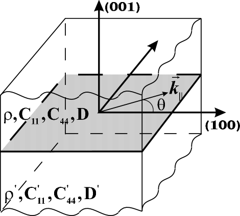
FIG. 1.: Structure for the study of interface acoustic waves.

The equations of motion (1) have to be supplemented by the boundary conditions on the interface, expressing continuity of the displacement and normal components of the stress tensor:

$$u_{i} = u_{i}^{\prime}\left|{}_{x_{3}=0}\right.,\quad i=1,2,3,$$ (5)

$$\sigma_{i3} = \sigma_{i3}^{\prime}\left|{}_{x_{3}=0},\right.\quad i=1,2,3\ .$$ (6)

The homogeneous plane waves (bulk phonons) are the simplest solutions of the wave equation in one infinite medium. They are

$${\bf u}^{(l)}({\bf r},t)=\exp\left(i{\bf k}_{\|}{\bf x}_{\|}+ik_{3}x_{3}-i\omega_{(l)}t\right)$$ (7)

for three different branches $l=1,2,3$, where ${\bf x}_{\|}$ and ${\bf k}_{\|}$ are two-dimensional vectors with components $(x_{1},x_{2},0)$ and $(k_{1},k_{2},0)\equiv k(\cos\theta,\sin\theta,0)$ respectively (the angle $\theta$ is counted from [100] direction), and $\omega_{(l)}=s_{(l)}\sqrt{k^{2}+k_{3}^{2}}$ with the bulk sound velocity $s_{(l)}=s_{(l)}(\theta,\phi)$, where $\cos\phi=k_{3}/\sqrt{k^{2}+k_{3}^{2}}$.

The solution for the phase velocity can be determined by substitution the plane wave of Eq. (7) into the equations of motion (1). It gives the homogeneous set of linear equations. Setting the determinant of the coefficients equal to zero, produces a cubic equation in $v^{2}$. Three roots of this equation are squares of the velocities for three bulk phonons.

For the propagation along (001) plane one of the velocities $t_{1}=\sqrt{C_{44}/\rho}$ is independent of $\theta$ and represents a transverse mode. Two others depend on angle of propagations in the plane. They are neither longitudinal nor transverse, but we denote the upper branch by the letter “$l$” and the lower one by “$t_{2}$”.

The interface between two half-infinite media introduces an inhomogeneity in $x_{3}$ direction. Therefore, we could expect that the plane waves also become inhomogeneous in this direction. The frequency and wave vector ${\bf k}_{\|}$ are the same in both media, but the component $k_{3}$ of wave vector may be complex and different in upper and lower media. Moreover, since boundary conditions Eqs.(5,6) comprise of 6 equations, the simplest solution for arbitrary direction of propagation should consist of linear superposition of three terms described by Eq. (7) for each medium with their own different complex components $k_{3}$.

The further analysis is facilitated by performing a rotation of the coordinate frame in such a way that the direction of propagation of the acoustic wave in the plane of interface is along the $x_{1}$ axis, i.e. ${\bf\tilde{k}}_{\|}=(k,0,0)$. Let

$$\hat{\mbox{\bf T}}=\left[\begin{array}[]{ccc}\cos\theta&\sin\theta&0\\ -\sin\theta&\cos\theta&0\\ 0&0&1\end{array}\right]$$ (8)

be the transformation matrix which produces this rotation. Then, the transformation law for the elements of the elastic modulus tensor under this rotation is

$$\tilde{\lambda}_{ijkl}=\sum_{i^{\prime}j^{\prime}k^{\prime}l^{\prime}}T_{ii^{\prime}}T_{jj^{\prime}}T_{kk^{\prime}}T_{ll^{\prime}}\lambda_{i^{\prime}j^{\prime}k^{\prime}l^{\prime}}.$$ (9)

At the first stage of the analysis we determine the possible values of $k_{3}$ for given magnitude of $k$. To this end, we define $k_{3}\equiv ik\beta$, $\omega=kv$ and we suggest the solution for the interface waves in the rotated system in the following form

$$u_{i} = A_{i}e^{-k\beta x_{3}}\exp\left[ik(x_{1}-vt)\right],\quad\mbox{for }x_{3}>0,$$ (10)

$$u_{i}^{\prime} = A_{i}^{\prime}e^{k\beta^{\prime}x_{3}}\exp\left[ik(x_{1}-vt)\right],\quad\mbox{for }x_{3}<0.$$ (11)

Conceptually, the $x_{3}$-dependence is the part of the “amplitude” (See Ref. [27]) and the wave-like properties are described by a common propagation part $\exp\left[ik(x_{1}-vt)\right]$. Thus, the propagation vector is always assumed to be parallel to the interface even though the exponent $\beta$ may be complex.

If Re$\beta,\beta^{\prime}>0$, then such a form describes a wave that propagates in $x_{1}$ direction, whose amplitudes decays exponentially with increasing distance into the medium from interface. The waves with (i) Re$\beta<0$ and Im$\beta<0$, (ii) Re$\beta^{\prime}<0$ and Im$\beta^{\prime}<0$, (iii) Re$\beta,\beta^{\prime}<0$ and Im$\beta,\beta^{\prime}<0$ are the leaky waves which radiate the energy outward the interface.

Substituting Eq.(9,11) into the equations of motion Eq. (1) yields the set of homogeneous equations for each media

$$L_{ij}(v,\beta)A_{j} = 0.$$ (12)

$$L^{\prime}_{ij}(v,\beta^{\prime})^{\prime}A_{j}^{\prime} = 0,$$ (13)

where matrix ${\bf L}$ (or ${\bf L}^{\prime}$) has the form

$$\left[\begin{array}[]{ccc}-C_{44}\beta^{2}+C_{11}-\frac{1}{2}D\sin^{2}2\theta-\rho v^{2}&-\frac{1}{4}D\sin 4\theta&\pm i\beta(C_{11}-C_{44}-D)\\ -\frac{1}{4}D\sin 4\theta&-C_{44}\beta^{2}+C_{44}+\frac{1}{2}D\sin^{2}2\theta-\rho v^{2}&0\\ \pm i\beta(C_{11}-C_{44}-D)&0&C_{44}-C_{11}\beta^{2}-\rho v^{2}\end{array}\right].$$ (14)

The sign plus (minus) corresponds to the upper (lower) medium, and we omitted primes for the lower medium. In each medium Eqs. (12) have nontrivial solutions if the corresponding determinant of the coefficients vanishes:

$${\rm det}({\bf L})=0,$$ (15)

It gives the secular equation on unknown values of $\beta$ with a phase velocity $v$ as a parameter. The explicit form of Eq. (15) is given in Appendix A. Due to the fact that we are seeking the solution for wave propagation in crystal plane of mirror symmetry this equation is bicubic in $\beta$ and the roots have inversion symmetry with respect to the origin of the complex plane[27]. One can also show that if $\beta_{l}={\beta_{R}}_{j}+i{\beta_{I}}_{j}$ at $j=1,\ldots,6$ are the roots of Eq. (15) with complex velocity $v=v_{R}+iv_{I}$, then the roots $\beta_{j}={\beta_{R}}_{j}-i{\beta_{I}}_{j}$ are the roots of the same equation with $v=v_{R}-iv_{I}$. Here the superscripts “$R$” and “$I$” denote the real and imaginary parts respectively.

The amplitudes $A_{\alpha}$ (or $A_{\alpha}^{\prime}$) for any $\beta_{j}$ ($\beta_{j}^{\prime}$) are related by

$$\frac{A_{1}^{(j)}}{C_{1}^{(j)}}=\frac{A_{2}^{(j)}}{C_{2}^{(j)}}=\frac{A_{3}^{(j)}}{C_{3}^{(j)}}=K_{j},\qquad j=1,\ldots,6,$$ (16)

where the ${K_{j}}$ are constants and $C_{\alpha}^{(j)}(v,\beta_{j})\ (\alpha=1,2,3)$ are the cofactors of the elements in the first row of the matrix L:

$$C_{1}^{(j)} = L_{22}L_{33},$$ (17)

$$C_{2}^{(j)} = -L_{21}L_{33},$$ (18)

$$C_{3}^{(j)} = -L_{31}L_{22}.$$ (19)

The next step of our analysis is a construction of the general solution, which satisfies boundary conditions Eq. (5,6). To this end, we form a linear combinations from three terms (11) with undefined constants $K_{j}$ and $K^{\prime}_{j}$ for each medium:

$$u_{\alpha} = \sum_{j=1}^{3}\frac{C_{\alpha}^{(j)}}{C_{1}^{(j)}}K_{j}\exp\left(ik(x_{1}-vt+i\beta_{j}(v)x_{3})\right),\quad\mbox{for }x_{3}>0,$$ (20)

$$u_{\alpha}^{\prime} = \sum_{j=1}^{3}\frac{C_{\alpha}^{\prime(j)}}{C_{1}^{\prime(j)}}K_{j}^{\prime}\exp\left(ik(x_{1}-vt-i\beta^{\prime}_{j}(v)x_{3})\right),\quad\mbox{for }x_{3}>0.$$ (21)

Substitution of this form for the displacement field into Eqs. (5, 6) leads to a set of 6 (in general case) homogeneous linear equations for the ${K_{j},K_{j}^{\prime}}$. The nontrivial solutions exist if the corresponding determinant vanishes:

$$|D_{kl}^{(\gamma)}(v)|=0,\quad k,l=1,\ldots,6.$$ (22)

Eq. (22) is the dispersion relation for the phase velocity $v$ of the interface acoustic wave. In general it has to be solved numerically. The left hand side function $D(v)\equiv|D_{kl}^{(\gamma)}|$ is some algebraic expression. Therefore, in general, the roots of Eq. (22) are complex. Moreover, since $D(v)$ comprises of six different decay constants $\beta_{j}(v),\beta^{\prime}_{j}$, which involve square roots from some expressions of $v^{2}$, the function $D(v)$ is multi-valued analytical function of complex variable $v$, defined on its associated Riemann sheets. The upper-script $\gamma$ enumerates these sheets. The number of Riemann sheets are determined by different combinations of $\beta$ branches. However, not all from $6!/3!3!=20$ combinations of $\beta_{j}$ are possible for each medium in the superpositions of Eq. (21). Each of three decay constants must be taken from the different roots $\beta^{2}$ of cubic equation ${\rm det}({\bf L})=0$ at fixed $v^{2}$. Therefore, the total number of possible combinations is $2^{3}\times 2^{3}=64$. This is the number of Riemann sheets for our case. Since simultaneous change of all signs $\beta,\beta^{\prime}$ in Eq. (22) does not change the form of determinant (see Appendix A), it is enough, in fact, to investigate 32 independent Riemann sheets in order to find all possible roots of the dispersion relation. In the isotropic case and for the propagation along the directions of high symmetry the number of independent Riemann sheets reduces to 8.

The sign convention for the sheets is determined by real part of $\beta$. It is denoted as follows:

$$\left(\mbox{sign}\mbox{Re}(\beta_{1}),\mbox{sign}\mbox{Re}(\beta_{2}),\mbox{sign}\mbox{Re}(\beta_{3}),\mbox{sign}\mbox{Re}(\beta^{\prime}_{1}),\mbox{sign}\mbox{Re}(\beta^{\prime}_{2}),\mbox{sign}\mbox{Re}(\beta^{\prime}_{3})\right).$$ (23)

Let us assume that $\gamma=1$ corresponds to the case (++++++). If a solution exists on this sheet, then it is a true interface wave, which is also called Stoneley wave. All other $\gamma$ correspond either leaky waves or non-physical solutions. Some of them may also correspond to bulk phonons (see section III). In the next section we formulate selection rules for physical solutions. The right direction of the energy flux is the main principle for the selection. The explicit form of Eq. (22) and the way of enumeration of its Riemann sheets are given in Appendix A.

III Selection rules for velocity and physical meaning of leaky waves

The question of total number of possible values of velocity has been investigated in earlier 70s theoretically[17] for the isotropic solid – liquid interface, and numerically for the case of two isotropic solids[7]. In the case of the liquid – solid interface there are eight Riemann sheets. It is shown[17] that the roots on all these sheets are the roots of an eight order polynomial in $v^{2}$ with real coefficients, and so there are eight complex roots which are either real or come in complex conjugate pairs. Numerical investigation of the Stoneley equation (A27) for isotropic solid – solid interface[7] has shown that there are sixteen independent roots on its sixteen Riemann sheets.

Thus, we can put forward a simple hypothesis: The number of possible values of $v^{2}$ is equal to the number of Riemann sheets. However, some of them may be degenerate so we are speaking about maximum number of different $v^{2}$. Note that this hypothesis is true for isotropic surface wave either. It follows from it that the maximum number of modes in our interface is 64. To check this hypothesis we have calculated this number for one of direction which does not have any special symmetry. The result is 64.

Let us turn now to the problem of roots classification for the case $\gamma>1$. First of all we discuss real roots for $v$ of the dispersion equation Eq. (22). If all $\beta$ are pure imaginary, it corresponds to refraction of bulk phonons and has nothing in common with leaky waves. If at least one of $\beta$ at any side has a negative real part, such solution should be considered as non-physical. If it happens that some $\beta$ are imaginary but some are complex with positive real part, then it relates to the problem of total internal reflection of bulk phonons. In numerical analysis we discard such solution, since they have a different nature.

Now we come to complex $v$. Let us assume that we have real positive frequency $\omega>0$ and complex root

$$v=v_{R}\mp iv_{I}$$ (24)

of the Eq. (22). As follows from Appendix A all complex roots form such pairs. Then, the wave vectors of propagation along $x_{1}$-axis for these solutions will be complex and equal to

$$k=\omega/v=\omega/(v_{R}\mp iv_{I})=k_{R}\pm ik_{I}.$$ (25)

If $k_{R}>0$, it corresponds to the running wave propagating from the left to the right with exponentially decreasing or increasing amplitudes. Since both of these solutions always meet in pairs we will consider only the wave attenuated from the left to the right. Then we should chose only the root $k_{R}+ik_{I}$ or $v_{R}-iv_{I}$, where $v_{R},v_{I},k_{R},k_{I}>0$.

Since $\gamma>1$, one or several $\beta$ have negative real part, i. e.

$$\beta=-\beta_{R}-i\beta_{I},$$ (26)

where $\beta_{R}>0$ and sign $\beta_{I}$ is not determined yet.

It is useful to introduce the following notations:

$$\tilde{v}_{R} = (v_{R}^{2}+v_{I}^{2})/v_{R},$$ (27)

$$\tilde{\beta}_{R} = \beta_{R}-\beta_{I}v_{I}/v_{R},$$ (28)

$$\tilde{\beta}_{I} = \beta_{I}+\beta_{R}v_{I}/v_{R},$$ (29)

After substitution $k=\omega/v$ the term has a form of inhomogeneous plane wave (see also the succeeded section)

$$e^{-i\omega(t-x/\tilde{v}_{R}-z\tilde{\beta}_{I}/\tilde{v}_{R})}e^{-\omega/\tilde{v}_{R}(xv_{I}/v_{R}-z\tilde{\beta}_{R})}.$$ (30)

In fact, the sign of $\beta_{I}$ is not arbitrary, but is dictated by the radiation condition[18, 19]. Indeed, since we consider here lossless media the only reason for the amplitude attenuation along direction of propagation on the interface is radiation of energy away from the interface into the bulk media. The total wave vector ${\bf q}=\omega/\tilde{v}_{R}(1,0,\tilde{\beta}_{I})$ is no longer parallel to the boundary, but is inclined to it, which indicates the presence of continuous flow of energy from the boundary to the bulk. Note that direction of phase propagation ${\bf q}/q$ does not represent the direction of energy flow itself. The later is determined by the time averaged power flux

$$W_{\alpha}=-{\hbox{Re}}\langle\frac{1}{2}\sigma_{\beta\alpha}\dot{u}_{\beta}^{*}\rangle,\qquad\alpha,\beta=1,2,3.$$ (31)

One can show that for small $v_{I}$ the sign of the component $W_{3}$ which determines the flow perpendicular to the interface coincides with the sign of $\tilde{\beta}_{I}$. Therefore, in notations of Eq. (26) the sign $\tilde{\beta}_{I}$ must be positive to guarantee the proper radiation condition.

Now we come to the physical meaning of the leaky waves. Discussing Rayleigh waves Landau and Lifshitz[10] prescribe to drop as non-physical the solution, which increases away from the surface. In the theory of leaky waves we take into consideration such a solution. The goal of this part is to give physical explanation of leaky waves (see also review by Maradudin [21]).

On both side of the interface our solution consists of three inhomogeneous plane waves. At large values of $x$ and $z$ these waves can be considered as independent. So we concentrate on one of them choosing the wave at $z>0$ with negative real part of $\beta$, i.e. the wave exponentially increasing with $z$. This wave has a form Eq. (30).

$$e^{-i\omega(t-x/\tilde{v}_{R}-z\tilde{\beta}_{I}/\tilde{v}_{R}})e^{-\omega/\tilde{v}_{R}(xv_{I}/v_{R}-z\tilde{\beta}_{R})},$$ (32)

where $\tilde{\beta}_{R}>0$ and $\tilde{\beta}_{I}>0$. This is an inhomogeneous bulk plane wave with wave vector ${\bf q}=\omega/\tilde{v}_{R}(1,0,\tilde{\beta}_{I})$ propagating away from the interface. The lines of constant phase are determined by the equation $t-x/\tilde{c}_{R}-z\tilde{\beta}_{I}/\tilde{c}_{R}=C_{1}$, and the lines of constant amplitude are given by the equation $xv_{I}/v_{R}-z\tilde{\beta}_{R}=C_{2}$ (See Fig. 2) The later expression shows that such modes attenuate when they move along the surface $z=0$.

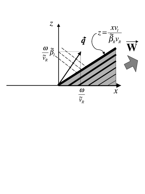
FIG. 2.: Illustration for geometry of leaky interface wave term. Power flux ${\bf W}$ and wave vector ${\bf q}$ are shown. The full lines with different thickness are the lines of a constant amplitude. The thickness of the lines indicates schematically the absolute value of the amplitudes. Dashed lines are the lines of a constant phase. For visual clarity the angle of constant amplitude lines has been exaggerated.

The central point of our understanding of the leaky waves is that one can not consider this waves in whole region of $x$, since amplitude becomes infinite when $x\longrightarrow-\infty$. This happens because we have chosen the solution which propagates from the left to the right along $x$-axis. Thus, we should propose that the wave creates at some line, say $x=0$, in the plane of the interface. Our equations of motion do not include any dissipation, therefore the attenuation in the plane of interface may be only due to radiation into the media. There is an important theorem [22] stating that for inhomogeneous plane waves the energy flux is parallel to the plane of constant amplitude. The cross-sections of these planes with the plane $zx$ are shown by full lines of different thickness. The upper line is thicker because the amplitude of the wave at the line $x=0$ is the largest and it decrease with increasing $x$. That is why the amplitude at any point $x$ increases with $z$ at $z<xv_{I}/\tilde{\beta}v_{R}$. It follows from the above theorem that the energy flux can not cross the planes of constant amplitude. It also can not cross the plane of maximal amplitude. This means that all the wave is within the wedge formed by the plane of interface and the plane of maximal amplitude $z=xv_{I}/\tilde{\beta_{R}}v_{R}$, at least in a sense that the whole energy of the wave is within this wedge. The amplitude of the wave is finite everywhere in this region.

One gets a severe contradiction considering a stationary problem. Indeed, the equation (32) gives nonzero result outside the wedge as well. Moreover amplitude diverges when $z$ tends to infinity. This is an artifact of the stationary consideration. The origin of the divergence is the infinite amplitude of the wave at point $x=-\infty$. The increase of the amplitude at large $z$ is an artifact originated from the flux coming from large negative $x$.

It is important to mention that the leaky wave does not differ substantially from the true interface wave only if $k_{R}\gg k_{I}$ in Eq. (18) or $v_{R}\gg v_{I}$. Since $\beta_{R}$ is not small, it means that the angle between the planes, forming the wage in Fig. 2, should be small. If this condition is not satisfied, the interface (or surface ) wave can not be considered as a wave since the wavelength is larger than the attenuation length.

The problem does not contain any small parameter which could make this condition fulfilled. The numerics show, however, that the majority of modes have small attenuation. The roots of this phenomenon are not clear for us.

Thus, based on discussion in this section we use the following selection rules for values $v=v_{R}-iv_{I}$, which are solutions of Eq. (22).

1. $v_{R}>0$, $v_{I}\geq 0$.

2. If $v_{I}=0$, than Re$\beta$, Re$\beta^{\prime}>0$.

3. If $v_{I}>0$ and Re$\beta<0$, than Im$\beta<0$.

4. If $v_{I}>0$ and Re$\beta^{\prime}<0$, than Im$\beta^{\prime}<0$.

IV Numerical results

To calculate velocities as a function of angle we use Eq. (A1) for $\beta^{2}$ and Eq. (A9). At the first step we divide complex plane $v$ in interval 2 km/s$<v_{R}<7$ km/s, $0<v_{I}<0.6$ km/s into 400 squares. For the vertex of each square we find six values of $\beta$ for upper medium and six values of $\beta^{\prime}$ for the lower medium using Eq. (A1). For each value of $v$ we find 32 different combinations of $\beta$ (each of 6 values) and substitute them into Eq. (A9). For each Riemann sheet $\gamma$ we find all minima of abs($|D_{ij}^{(\gamma)}(v)|$) with respect to $v_{R}$ and $v_{I}$ using a standard program. For those minima which are close to zero, we do iterative search of roots. The parameters of the bulk lattices have been taken from the Table I. TABLE I.: Densities(g/cm³), elastic constants ($10^{10}$N/m²), and sound velocities (km/s) in the directions of high symmetry for bulk crystals[20]. Crystal $\rho$ $C_{11}$ $C_{12}$ $C_{44}$ $l_{[100]}$ $t_{1}$ $l_{[110]}$ $t_{2[110]}$ Al_0.3Ga_0.7As 4.794 12.24 5.65 5.90 5.05 3.51 5.56 2.62 GaAs 5.307 12.26 5.71 6.0 4.81 3.36 5.31 2.48 To check the method some results have been obtained using completely different Surface Green Function Matching method[23, 25], which is discussed in Appendix B. We have not found any differences between the results of two methods.

For an additional check of the problem we have calculated true surface waves for both materials. The dispersion relation for surface waves on (001) cut of cubic crystals can be obtained from the determinant of truncated interface matrix Eq. (A8). For the upper (lower) medium we should take lower left (right) 3x3 part of the matrix. We have gotten 2.873 km/s (2.737 km/s) for GaAs (Al_0.3Ga_0.7As). These results may be compared with the results by Farnell[27] Our results are slightly different because of the difference in the parameters of bulk materials. Taking parameters used by Farnell we have obtained his velocities with a very high accuracy.

The results for leaky interface waves are shown in Fig. 3 and Fig. 4. Plotting this figure we have taken into account all selection rules formulated at the end of section III. The discontinuities appear because at some points these rules are not fulfilled and the corresponding modes become non-physical. All the modes have different anisotropy, different attenuation and different angle intervals of their existence. In Fig.3 we draw all the modes (Note that velocity scales in 3(a) and 3(b) are different). One can see that there are abundant number of leaky interface modes in the velocity range between 3km/s and 4km/s. Thorough analysis shows however that a majority of those modes exists in a very restricted range of the angles. Probably, it will be difficult to detect them experimentally. In Figure 4 we draw selected modes which exist in the large interval of the angles only. We left one mode (A) with a small angle range in the figure as a typical example of discarded modes. For further clarification of the picture we also discard all physical modes with a strong anisotropy of their real and/or imaginary parts of the velocity. One of such modes with strong real part anisotropy (B) is left in the figure as an example.

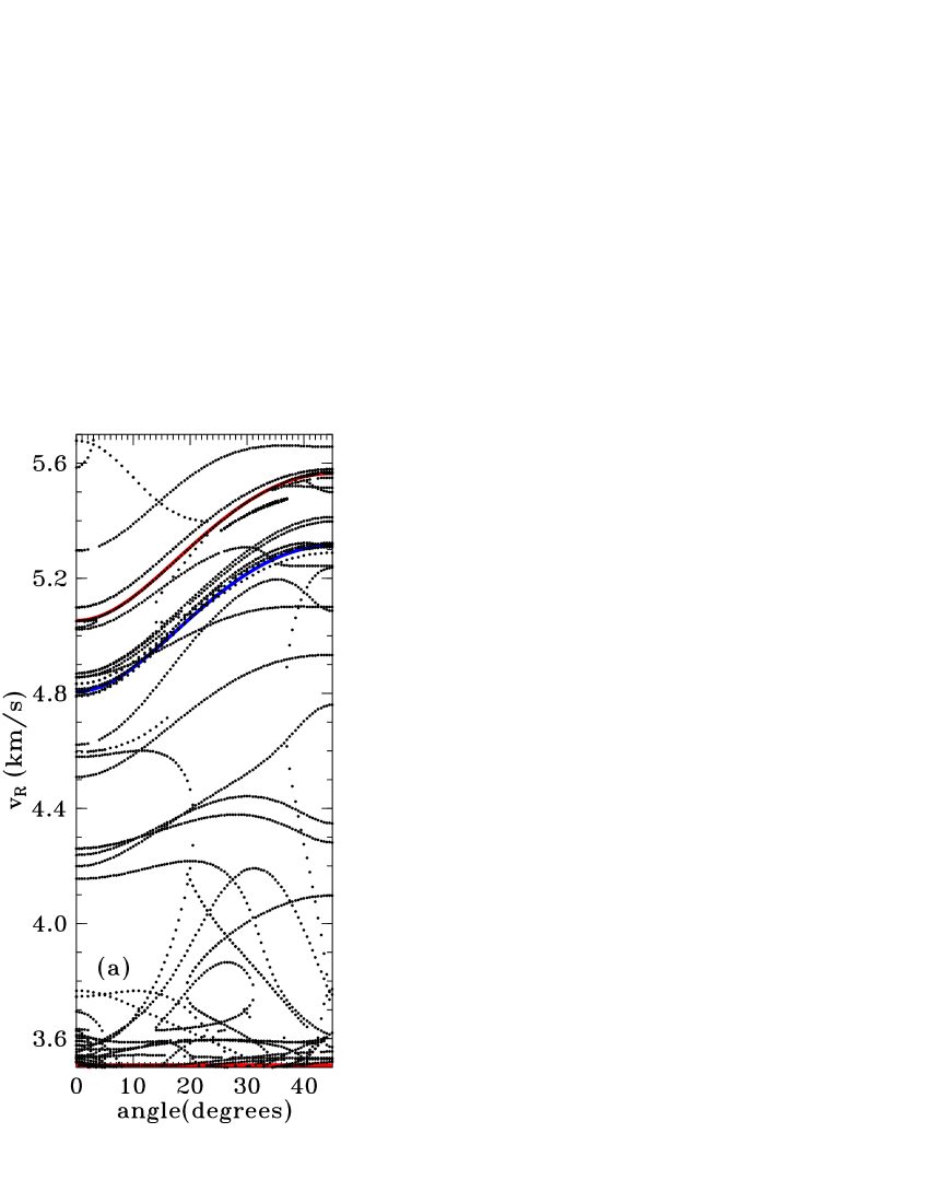
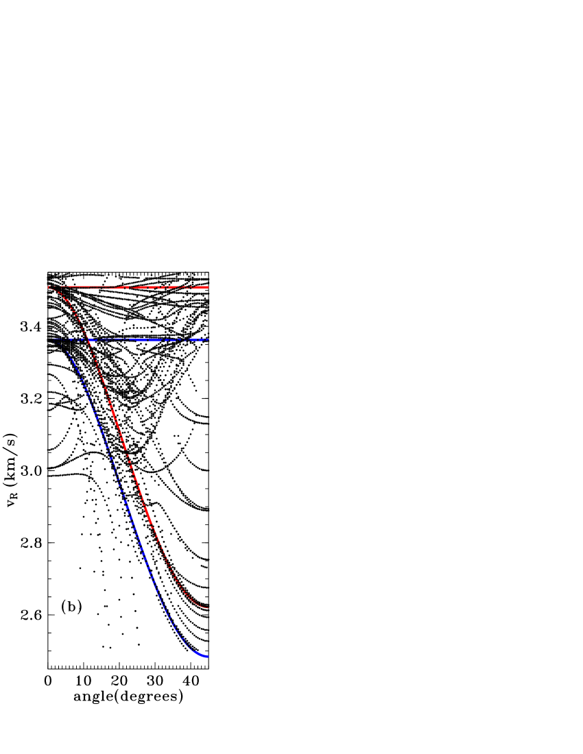
FIG. 3.: The real parts of complex velocities for all leaky interface waves in the range 3.5 km/s $<v_{R}<$ 5.7 km/s (a) and 2.4 km/s $<v_{R}<$ 3.5 km/s (b). The solid lines present velocities of bulk acoustic waves for both media.

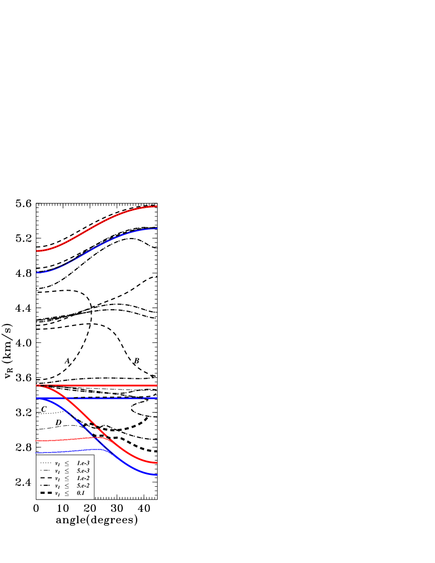
FIG. 4.: The real parts of complex velocities for the selected modes in the range 2.4 km/s $<v_{R}<$ 5.7 km/s. See explanation in the text. The numerical parameters for these modes are given in the Table II. The value of attenuation is determined by the imaginary part of complex velocity. Different linestyles and thickness correspond to different magnitude of average imaginary part $\overline{v_{I}}$ (km/s) of velocity. The solid lines present velocities of bulk acoustic waves and the dotted lines are true surface acoustic waves for both media (Upper curves correspond to Al_0.3Ga_0.7As and lower curves correspond to GaAls).

All numerical parameters for the modes presented in Fig. 4 are given in the table II. For modes classification we introduce the following parameters.

1. Averaged over angles real $\overline{v_{R}}$ and imaginary $\overline{v_{I}}$ part of the velocity.

2. Angle range parameter $\delta_{an}=(\varphi_{\max}-\varphi_{\min})\,4/\pi$. It equals to unity when a mode exists on whole range of angles and less than one otherwise.

3. Anisotropy parameters for real and imaginary parts of the velocity

   $$\sigma_{v_{R}}=(v_{R\max}-v_{R\min})/\overline{v_{R}},\qquad\sigma_{v_{I}}=(v_{I\max}-v_{I\min})/\overline{v_{I}}.$$ (33)

   Modes with smaller anisotropy have smaller $\sigma$.

Among the modes there are two (C and D in the figure) which remind those in the surface acoustic problem. Namely, for Al_xGa_1-xAs materials there are always[27] true SAWs (they are shown by dotted lines in the figure), which change very a little with angle until they meet the lowest bulk transverse velocity curves (they are shown by solid line). After that point the true SAWs repeat behavior of their bulk velocity curves up to the end - 45 degrees angle on the picture. Meanwhile, in the region between two transverse bulk velocity curves the leaky surface acoustic waves appear with approximately the same real part of velocity.

The situation for interface waves is different. As we mentioned, there are no true interface waves. However, there are leaky interface waves with a very small attenuation at small angles before “colliding” with the bulk transverse velocity curve. At larger angles the leaky modes acquire larger imaginary part of the velocity and become stronger attenuated (See Table II).

V
Conclusion

We have derived a dispersion equation for interface waves at the interface of two cubic crystals in the plane, perpendicular to [001]. Analyzing different solutions for the interface waves we come to conclusion that the total amount of interface modes in each direction is equal to the number of the Riemann sheets. In our case this is 64. We have successfully checked this hypothesis by calculating the number of modes in one direction of the interface plane, which does not have any special symmetry.

The computations have been made for the interface Al_0.3Ga_0.7As/GaAs. We have shown that in this case all interface modes, which have physical meaning are leaky, but majority of them have small attenuation in the direction of propagation. We show that for understanding of the physical meaning of leaky waves one should consider not a stationary problem , but the problem starting with creation of the wave at some line in the interface plane.

After that we are able to formulate how to separate this 64 modes into physical and non-physical modes. This separation mainly based upon some theorems on the energy flux and upon an assumption that if a mode deviates from the interface in some medium, the energy flux should go in the same medium.

Using the elastic moduli of the bulk lattices we have performed numerical calculations of the velocities of the interface waves as a function of an angle in the plane of interface in a wide range of velocities. The results are shown in Fig. 3. One can see two close groups of modes within the intervals 3$-$3.5 km/s and 4.2$-$4.5 km/s respectively. These groups may be responsible for two periods of oscillations which have been observed in the experiment with the two-dimensional electron gas in magnetic field[16], mentioned in the introduction. Note that the velocities of the leaky interface waves may be sensitive to the difference of the bulk media parameters. This difference is not known good enough. This fact may be responsible for possible deviation of our calculations from the experimental data.

VI Acknowledgments

The authors wish to thank B. Bromley for the helpful advises. IVP is grateful to V. Velasco for giving his numerical source code for calculations of Stoneley waves which was valuable check for our method. This work was supported by Seed grant of the University of Utah.

TABLE II.: Parameters for the selected modes. The units for average velocities are km/s.

$\#$	$\delta_{an}$	$\overline{v_{R}}$	$\overline{v_{I}}$	$\sigma_{v_{R}}$	$\sigma_{v_{I}}$	$v_{R\min}$	$v_{R\max}$	$v_{I\min}$	$v_{I\max}$
$A$	0.46	4.166	6.5$\times 10^{-3}$	0.25	0.39	3.58	4.60	5.2$\times 10^{-3}$	7.7$\times 10^{-3}$
$B$	0.99	4.022	9.5$\times 10^{-3}$	0.15	2.48	3.60	4.22	2.1$\times 10^{-4}$	2.4$\times 10^{-2}$
$C_{1}$	0.26	3.195	1.9$\times 10^{-4}$	0.01	2.65	3.18	3.22	1.8$\times 10^{-11}$	5.1$\times 10^{-4}$
$C_{2}$	0.73	3.000	3.3$\times 10^{-2}$	0.10	2.50	2.89	3.19	3.8$\times 10^{-7}$	8.4$\times 10^{-2}$
$D_{1}$	0.63	2.966	5.3$\times 10^{-3}$	0.11	1.00	2.72	3.05	1.9$\times 10^{-3}$	7.2$\times 10^{-3}$
$D_{2}$	0.53	2.856	6.6$\times 10^{-2}$	0.07	2.76	2.75	2.95	2.3$\times 10^{-4}$	0.18
1	1	5.369	7.9$\times 10^{-3}$	0.09	1.32	5.10	5.58	3.4$\times 10^{-3}$	1.4$\times 10^{-2}$
2	1	5.167	4.2$\times 10^{-3}$	0.1	0.31	4.83	5.32	3.7$\times 10^{-3}$	5.0$\times 10^{-3}$
3	1	5.330	2.1$\times 10^{-4}$	0.1	3.44	5.05	5.56	2.2$\times 10^{-6}$	7.1$\times 10^{-4}$
4	1	5.112	6.8$\times 10^{-3}$	0.09	0.79	4.86	5.32	4.1$\times 10^{-3}$	9.4$\times 10^{-3}$
5	1	5.115	4.0$\times 10^{-3}$	0.1	0.19	4.83	5.32	3.7$\times 10^{-3}$	4.5$\times 10^{-3}$
6	1	5.104	3.5$\times 10^{-2}$	0.1	1.41	4.81	5.32	9.5$\times 10^{-3}$	5.9$\times 10^{-2}$
7	1	4.960	3.5$\times 10^{-2}$	0.12	1.72	4.62	5.20	1.6$\times 10^{-2}$	7.7$\times 10^{-2}$
8	1	4.446	8.7$\times 10^{-3}$	0.13	1.75	4.20	4.76	2.6$\times 10^{-3}$	1.8$\times 10^{-2}$
9	1	4.360	2.1$\times 10^{-2}$	0.05	0.65	4.24	4.44	1.3$\times 10^{-2}$	2.7$\times 10^{-2}$
10	1	4.323	2.2$\times 10^{-2}$	0.03	0.58	4.26	4.38	1.4$\times 10^{-2}$	2.7$\times 10^{-2}$
11	0.94	3.578	2.0$\times 10^{-2}$	0.02	2.22	3.53	3.60	1.2$\times 10^{-3}$	4.6$\times 10^{-2}$
12	0.99	3.475	3.1$\times 10^{-3}$	0.02	1.27	3.45	3.51	2.0$\times 10^{-4}$	4.1$\times 10^{-3}$
13	0.99	3.452	3.1$\times 10^{-2}$	0.03	1.63	3.42	3.51	2.0$\times 10^{-4}$	5.1$\times 10^{-2}$
14	0.68	3.77	8.8$\times 10^{-3}$	0.01	1.35	3.37	3.42	8.6$\times 10^{-4}$	1.3$\times 10^{-2}$
15	0.99	3.79	4.1$\times 10^{-2}$	0.11	1.46	3.15	3.51	2.0$\times 10^{-4}$	5.9$\times 10^{-2}$
16	0.53	3.040	6.9$\times 10^{-2}$	0.05	1.69	3.00	3.15	1.0$\times 10^{-3}$	0.12

A Explicit form of the Dispersion relation in general, symmetry directions, and isotropic cases

From the determinant (15) we obtain the following equation on unknown variable $\beta$ with a phase velocity $v$ as a parameter:

$$\beta^{6}-\beta^{4}\left[a+b+c-\frac{(\lambda^{2}-1-d)^{2}}{\lambda^{2}}\right]+\beta^{2}\left[ab+bc+ca-b\frac{(\lambda^{2}-1-d)^{2}}{\lambda^{2}}-\tau^{2}\right]+c(\tau^{2}-ab)=0,$$ (A1)

where

$$a = \lambda^{2}\left(1-\frac{v^{2}}{\lambda^{2}t^{2}}\right)-\frac{d}{2}\sin^{2}2\theta,$$ (A2)

$$b = 1-\frac{v^{2}}{t^{2}}+\frac{d}{2}\sin^{2}2\theta,$$ (A3)

$$c = \frac{1}{\lambda^{2}}\left(1-\frac{v^{2}}{t^{2}}\right),$$ (A4)

$$\tau = \frac{d}{4}\sin 4\theta.$$ (A5)

“Weight factors” in Eq. (21) have the following form:

$$\frac{C_{\alpha}^{(j)}}{C_{1}^{(j)}}=\left\{\begin{array}[]{cc}1,&\quad\mbox{for }\alpha=1,\\ -\frac{L_{21}}{L_{22}}\equiv p_{2}^{(j)}(\beta_{j}^{2})=\frac{D/4\sin 4\theta}{-C_{44}\beta_{j}^{2}+C_{44}+D/2\sin^{2}\theta-\rho v^{2}},&\quad\mbox{for }\alpha=2,\\ -\frac{L_{31}}{L_{33}}\equiv\mp i\beta_{j}p_{3}^{(j)}(\beta_{j}^{2})=\mp i\beta_{j}\frac{C_{11}-C_{44}-D}{C_{44}-C_{11}\beta_{j}^{2}-\rho v^{2}},&\quad\mbox{for }\alpha=3,\end{array}\right.$$ (A6)

where the upper sign is for the upper medium, and for a convenience sake we omitted primes in formulae for the lower medium. Then, for each term in the sum (21) the condition (6) on the stress continuity in rotated frame can be written in the vector form:

$$\left[\begin{array}[]{c}\sigma_{13}^{j}\\ \sigma_{23}^{j}\\ \sigma_{33}^{j}\end{array}\right]=i\left[\begin{array}[]{ccc}\pm i\beta_{j}C_{44}&0&C_{44}\\ 0&\pm i\beta_{j}C_{44}&0\\ C_{12}&0&\pm i\beta_{j}C_{11}\end{array}\right]\ \left[\begin{array}[]{c}1\\ p_{2}^{(j)}\\ \mp i\beta_{j}p_{3}^{(j)}\end{array}\right].$$ (A7)

One can can see that the boundary conditions decouple for the sagittal plane $\left\{x_{1}x_{3}\right\}$ and the perpendicular direction $x_{2}$. With the help of Eq. (A7) and minor simplifications we obtain six homogeneous linear equations for the boundary conditions with the matrix ${\bf D}(v)$ equals to

$$\left[\begin{array}[]{cccccc}1&1&1&-1&-1&-1\\ p_{2}^{(1)}&p_{2}^{(2)}&p_{2}^{(3)}&-p_{2}^{\prime(1)}&-p_{2}^{\prime(2)}&-p_{2}^{\prime(3)}\\ \beta_{1}p_{3}^{(1)}&\beta_{2}p_{3}^{(2)}&\beta_{3}p_{3}^{(3)}&\beta_{1}^{\prime}p^{\prime}_{3}{{}^{(1)}}&\beta_{2}^{\prime}p_{3}^{\prime(2)}&\beta_{3}^{\prime}p_{3}^{\prime(3)}\\ C_{44}\beta_{1}p_{2}^{(1)}&C_{44}\beta_{2}p_{2}^{(2)}&C_{44}\beta_{3}p_{2}^{(3)}&C^{\prime}_{44}\beta^{\prime}_{1}p_{2}^{\prime(1)}&C^{\prime}_{44}\beta^{\prime}_{2}p_{2}^{\prime(2)}&C^{\prime}_{44}\beta^{\prime}_{3}p_{2}^{\prime(3)}\\ C_{44}\beta_{1}(1-p_{3}^{(1)})&C_{44}\beta_{2}(1-p_{3}^{(2)})&C_{44}\beta_{3}(1-p_{3}^{(3)})&C^{\prime}_{44}\beta^{\prime}_{1}(1-p_{3}^{\prime(1)})&C^{\prime}_{44}\beta^{\prime}_{2}(1-p_{3}^{\prime(2)})&C^{\prime}_{44}\beta^{\prime}_{3}(1-p_{3}^{\prime(3)})\\ C_{12}+C_{11}\beta_{1}^{2}p_{3}^{(1)}&C_{12}+C_{11}\beta_{2}^{2}p_{3}^{(2)}&C_{12}+C_{11}\beta_{3}^{2}p_{3}^{(3)}&-C^{\prime}_{12}-C^{\prime}_{11}\beta_{1}^{\prime 2}p_{3}^{\prime(1)}&-C^{\prime}_{12}-C^{\prime}_{11}\beta_{2}^{\prime 2}p_{3}^{\prime(2)}&-C^{\prime}_{12}-C^{\prime}_{11}\beta_{3}^{\prime 2}p_{3}^{\prime(3)}\end{array}\right].$$ (A8)

The condition for a nontrivial solution is that its determinant must vanish:

$$D^{(\gamma)}(v;\beta_{1},\ldots,\beta^{\prime}_{3})\equiv|D^{(\gamma)}_{ij}|=0.$$ (A9)

Since each $\beta$ is doubled value function of complex variable $v$, this determinant has 64 Riemann sheets, which we denote by upper-script $\gamma$.

The sign convention for independent sheets is determined by real part of $\beta$. It is given as follows:

$$\mbox{sign}\left(\mbox{Re}(\beta_{1}),\mbox{Re}(\beta_{2}),\mbox{Re}(\beta_{3}),\mbox{Re}(\beta^{\prime}_{1}),\mbox{Re}(\beta^{\prime}_{2}),\mbox{Re}(\beta^{\prime}_{3}),\right).$$ (A10)

That is, Riemann sheet (+ + + - - -) corresponds to the case Re$(\beta_{j})>0$ and Re$(\beta^{\prime}_{j})<0$, where $j=1,2,3$.

The important property of the determinant is that its solutions are invariant against the simultaneous change of sign of all six decay constants. Indeed, the functions $p_{2},\ p_{3}$ are defined in such a way that they depend on $\beta^{2}$ only. Therefore, from the form of matrix (A8) it follows that simultaneous change of sign $\beta$ leaves the secular equation unaltered. Thus, in order to find all the roots of Eq. (A9) it is enough to investigate only 32 independent Riemann sheets. To enumerate these sheets we, firstly, solve equation (A1) and sort obtained $\beta(v)$ for each medium in the following order:

$\displaystyle|\mbox{Re}(\beta_{1})|\leq|\mbox{Re}(\beta_{2})|\leq|\mbox{Re}(\beta_{3})|.$

Secondly, we choose notation that the sign of the real part $\beta_{1}$ is always positive. Then the upper Riemann sheet $\gamma=1$ corresponds to the case (++++++) and the subsequent numbers for lower sheets are given in the table III. $\gamma$ Re$\beta_{1}$ Re$\beta_{2}$ Re$\beta_{3}$ Re$\beta^{\prime}_{1}$ Re$\beta^{\prime}_{2}$ Re$\beta^{\prime}_{3}$ 1 + + + + + + 2 + + + + + - 3 + + + + - + 4 + + + - + + 5 + + + + - - 6 + + + - + - 7 + + + - - + 8 + + + - - - 9 + + - + + + $\cdots$ $\cdots$ $\cdots$ $\cdots$ $\cdots$ $\cdots$ $\cdots$ 17 + - + + + + $\cdots$ $\cdots$ $\cdots$ $\cdots$ $\cdots$ $\cdots$ $\cdots$ 25 + - - + + + $\cdots$ $\cdots$ $\cdots$ $\cdots$ $\cdots$ $\cdots$ $\cdots$ 32 + - - - - -

Another feature of Eq. (A9) is the following. If $v=v_{R}+iv_{I}$ is the solution of the dispersion relation $D^{(\gamma)}(v)\equiv D_{R}^{(\gamma)}+iD^{(\gamma)}_{I}=0$, then $v=v_{R}-iv_{I}$ will be also a solution of Eq. (A9). Here we explicitly separated real and imaginary part of complex function. It could be understood by the following consideration. Let $\beta_{l}=\beta_{R_{l}}+i\beta_{I_{l}}(l=1,\ldots,6)$, obtained from Eqs. (15) for $v=v_{R}+iv_{I}$, then the solutions of Eqs. (15) for $v=v_{R}-iv_{I}$ are $\beta_{l}=\beta_{R_{l}}-i\beta_{I_{l}}$. Moreover, the simultaneous change $v\longrightarrow v_{R}-iv_{I}$, $\beta_{l}\longrightarrow\beta_{R_{l}}-i\beta_{I_{l}}$ in Eq. (A9) brings up the change of sign at the imaginary part of the determinant only:

$\displaystyle D^{(\gamma)}(v_{R}-iv_{I})=D^{(\gamma)}_{R}-iD^{(\gamma)}_{I}.$

Thus $v=v_{R}-iv_{I}$ is also the solution.

If we suggest that frequency of the interface acoustic wave is real, then $k=\omega/v$ will be complex. We will choose solutions with $v=v_{R}-iv_{I}$ which correspond to the attenuated waves (for $\omega>0$) along direction of its propagation on the interface.

The dispersion relation simplifies considerably for the propagation on the interface (001) along the directions of high symmetry ([100] and [110]) and in the isotropic case. For all this cases, matrix elements $L_{12}=L_{21}\equiv 0$ [because of $\sin 4\theta=0$ or $D=0$, see Eq. (14)]. Therefore, the systems (12) for each media breaks up into the pair:

$$\left[\begin{array}[]{cc}L_{11}&L_{13}\\ L_{13}&L_{33}\end{array}\right]\left[\begin{array}[]{c}A_{1}\\ A_{3}\end{array}\right]=0$$ (A11)

and

$$L_{22}A_{2}=0.$$ (A12)

The only nontrivial solution of the latter corresponds to a bulk transverse acoustic wave propagating parallel to the interface of the elastic media [21], and therefore it is discarded. Thus, in these cases the interface waves polarized in the sagittal plane and do not have $u_{2}$ component.

For the interface waves polarized in the sagittal plane the solvability condition for (A11) is the biquadratic equation

$$\lambda^{2}\beta^{4}-\beta^{2}\left(\gamma_{1}^{2}+\lambda^{4}\gamma_{2}^{2}-(\lambda^{2}-1-d)^{2}\right)+\lambda^{2}\gamma_{1}^{2}\gamma_{2}^{2}=0,$$ (A13)

where we introduced notation

$$\lambda^{2} = C_{11}/C_{44},$$ (A14)

$$d = D/C_{44},$$ (A15)

$$\gamma_{1}^{2} = 1-v^{2}/t^{2},$$ (A16)

$$t^{2} = C_{44}/\rho,$$ (A17)

and

$$\gamma_{2}^{2}=\left\{\begin{array}[]{cc}1-v^{2}/(\lambda t)^{2}&\quad\mbox{for }\theta=0,\\ 1-d/2\lambda^{2}-v^{2}/(\lambda t)^{2}&\quad\mbox{for }\theta=\pi/4.\end{array}\right.$$ (A18)

In the isotropic case ($d=0$) the Eq. (A13) reduces to the

$$\beta^{4}-\beta^{2}\left(\gamma_{1}^{2}+\gamma_{2}^{2}\right)-\gamma_{1}^{2}\gamma_{2}^{2}=0$$ (A19)

with obvious solutions

$$\beta_{1} = \pm\sqrt{1-v^{2}/t^{2}}$$ (A20)

$$\beta_{2} = \pm\sqrt{1-v^{2}/(\lambda t)^{2}}.$$ (A21)

For all these cases the general solution for the interface wave are linear combinations of two partial waves for both media:

$$u_{1}({\bf r},t) = \left[K_{1}e^{-k\beta_{1}x_{3}}+K_{2}e^{-k\beta_{2}x_{3}}\right]e^{ik(x_{1}-vt)},$$ (A22)

$$u_{3}({\bf r},t) = \left[K_{1}p_{3}^{(1)}e^{-k\beta_{1}x_{3}}+K_{2}p_{3}^{(2)}e^{-k\beta_{2}x_{3}}\right]e^{ik(x_{1}-vt)},$$ (A23)

$$u^{\prime}_{1}({\bf r},t) = \left[K^{\prime}_{1}e^{k\beta^{\prime}_{1}x_{3}}+K^{\prime}_{2}e^{k\beta^{\prime}_{2}x_{3}}\right]e^{ik(x_{1}-vt)},$$ (A24)

$$u^{\prime}_{3}({\bf r},t) = \left[K^{\prime}_{1}p_{3}^{\prime(1)}e^{k\beta^{\prime}_{1}x_{3}}+K^{\prime}_{2}p_{3}^{\prime(2)}e^{k\beta^{\prime}_{2}x_{3}}\right]e^{ik(x_{1}-vt)}.$$ (A25)

After substitution solution (A22) into the boundary conditions (5,6) we obtain the set of four homogeneous linear equations with solvability condition:

$$\left|\begin{array}[]{cccc}1&1&-1&-1\\ \beta_{1}p_{3}^{(1)}&\beta_{2}p_{3}^{(2)}&\beta_{1}^{\prime}p_{3}^{\prime(1)}&\beta_{2}^{\prime}p_{3}^{\prime(2)}\\ C_{44}\beta_{1}(1-p_{3}^{(1)})&C_{44}\beta_{2}(1-p_{3}^{(2)})&C^{\prime}_{44}\beta^{\prime}_{1}(1-p_{3}^{\prime(1)})&C^{\prime}_{44}\beta^{\prime}_{2}(1-p_{3}^{\prime(2)})\\ C_{12}+C_{11}\beta_{1}^{2}p_{3}^{(1)}&C_{12}+C_{11}\beta_{2}^{2}p_{3}^{(2)}&-C^{\prime}_{12}-C^{\prime}_{11}\beta_{1}^{\prime 2}p_{3}^{\prime(1)}&-C^{\prime}_{12}-C^{\prime}_{11}\beta_{2}^{\prime 2}p_{3}^{\prime(2)}\end{array}\right|=0.$$ (A26)

For isotropic case $p_{3}^{(1)}=-1/\beta_{1}^{2}$ and $p_{3}^{(2)}=-1$. Then the resulting dispersion relation reduces[3] to

$$v^{4}\left[(\rho-\rho^{\prime})^{2}-(\rho\beta^{\prime}_{2}+\rho^{\prime}\beta_{2})(\rho\beta^{\prime}_{1}+\rho^{\prime}\beta_{1})\right]+4Fv^{2}\left[\rho\beta^{\prime}_{1}\beta^{\prime}_{2}-\rho^{\prime}\beta_{1}\beta_{2}-\rho+\rho^{\prime}\right]+4F^{2}(1-\beta_{1}\beta_{2})(1-\beta^{\prime}_{1}\beta^{\prime}_{2})=0,$$ (A27)

where

$$F=\rho t^{2}-\rho^{\prime}t^{\prime 2}.$$ (A28)

There are sixteen independent roots on eight different Riemann sheets for the given equation There is always non-attenuated solution for $t=t^{\prime}$, $\lambda=\lambda^{\prime}$ and $\rho\neq\rho^{\prime}$.

B GFSM method

In addition to our method described above it is also possible to obtain the dispersion relation for the interface wave using Surface Green Function Matching (SGFM) analysis (see for details Refs. [23, 24]). We used this technique as a complementary independent method in our numerical calculations to compare the results. The main advantage of the method is that it gives the determinant of the matrix with dimensions 3x3, rather than 6x6. However, the calculation of the those matrix elements is more cumbersome. Another important development of this method is construction of the Green function of whole system, which also enables to calculate interface contribution to the important physical properties of the system such as the density of phonon modes, specific heat, and the atom mean square displacements.

We consider the (001) interface of cubic crystals and arbitrary propagation directions. The idea of the method is to construct the Green function G^s of the composite two-media system, such that it incorporates the boundary conditions at the interface. In fact, to obtain the dispersion relation it suffices to know the surface projection ${\bf g^{s}}$ of G^s on the interface plane. Since the boundary conditions (5,6) involve first derivatives, the surface projection of the bulk Green functions ${\cal G}_{ij}$ and their normal derivatives will be involved. These are defined by

$$G_{ij} = \lim_{x_{3}^{\prime}\rightarrow 0}\left[\langle x_{3}|{\cal G}_{ij}|x_{3}^{\prime}\rangle\right]_{x_{3}=0}=\lim_{\eta\rightarrow 0}\frac{1}{2\pi}\int_{-\infty}^{\infty}{\cal G}_{ij}(q)\exp(iq\eta)\,dq,$$ (B1)

$$G_{ij}^{(\pm)} = \lim_{x_{3}^{\prime}\rightarrow\pm 0}\left[\frac{\partial\langle x_{3}|{\cal G}_{ij}|x_{3}^{\prime}\rangle}{\partial x_{3}}\right]_{x_{3}=0}=\lim_{\eta\rightarrow 0}\frac{1}{2\pi}\int_{-\infty}^{\infty}{\cal G}_{ij}(q)iq\exp(\mp iq\eta)\,dq.$$ (B2)

In our case ${\bf{\cal G}}(q)=\left[{\bf L}\right]^{-1}$, where matrix L is given by Eq. (14) with substitution $i\beta\rightarrow q$. The calculation is tedious but straightforward[30].

$$G_{11} = \sum_{j=1}^{3}\frac{(\gamma_{1}^{2}-\beta_{j}^{2}\lambda^{2})(\gamma_{1}^{2}+\frac{d}{2}\sin^{2}2\theta-\beta_{j}^{2})}{2\lambda^{2}\beta_{j}(\beta_{j+1}^{2}-\beta_{j}^{2})(\beta_{j+2}^{2}-\beta_{j}^{2})C_{44}},$$ (B3)

$$G_{22} = \sum_{j=1}^{3}\frac{(\gamma_{1}^{2}-\lambda^{2}\beta_{j}^{2})(\lambda^{2}-\frac{v^{2}}{t^{2}}-\frac{d}{2}\sin^{2}2\theta-\beta_{j}^{2})+\beta_{j}^{2}(\lambda^{2}-1-d)^{2}}{2\lambda^{2}\beta_{j}(\beta_{j+1}^{2}-\beta_{j}^{2})(\beta_{j+2}^{2}-\beta_{j}^{2})C_{44}},$$ (B4)

$$G_{33} = \sum_{j=1}^{3}\frac{(\gamma_{1}^{2}-\beta_{j}^{2})(\lambda^{2}-\frac{v^{2}}{t^{2}}-\beta_{j}^{2})+\frac{d}{2}\sin^{2}2\theta(-\frac{d}{2}+\lambda^{2}-1)}{2\lambda^{2}\beta_{j}(\beta_{j+1}^{2}-\beta_{j}^{2})(\beta_{j+2}^{2}-\beta_{j}^{2})C_{44}},$$ (B5)

$$G_{12} = {G}_{21}=\frac{d\tau}{2\lambda^{2}}\sum_{j=1}^{3}\frac{\lambda^{2}\beta_{j}^{2}-\gamma_{1}^{2}}{\beta_{j}(\beta_{j+1}^{2}-\beta_{j}^{2})(\beta_{j+2}^{2}-\beta_{j}^{2})C_{44}},$$ (B6)

$$G_{13} = G_{31}=G_{23}=G_{32}=0;$$ (B7)

$$G_{11}^{(\pm)} = G_{22}^{(\pm)}=\pm\frac{1}{2C_{44}},$$ (B8)

$$G_{33}^{(\pm)} = \pm\frac{1}{2C_{11}},$$ (B9)

$$G_{12}^{(\pm)} = G_{21}^{(\pm)}=0,$$ (B10)

$$G_{13}^{(\pm)} = G_{31}^{(\pm)}=-\frac{i(\lambda^{2}-1-d)}{2\lambda^{2}C_{44}}\sum_{j=1}^{3}\frac{\left[\beta_{j}^{2}-(1+\frac{d}{2}\sin^{2}2\theta)+\frac{v^{2}}{t^{2}}\right]\beta_{j}}{(\beta_{j+1}^{2}-\beta_{j}^{2})(\beta_{j+2}^{2}-\beta_{j}^{2})},$$ (B11)

$$G_{23}^{(\pm)} = G_{32}^{(\pm)}=-\frac{id\tau(\lambda^{2}-1-d)}{2\lambda^{2}C_{44}}\sum_{j=1}^{3}\frac{\beta_{j}}{(\beta_{j+1}^{2}-\beta_{j}^{2})(\beta_{j+2}^{2}-\beta_{j}^{2})}.$$ (B12)

Here $\theta$ is the angle formed by the direction of propagation and the $x_{1}$ axis, $\tau=-\frac{\sin 4\theta}{4}$ and notations for $\lambda,d,\gamma_{1},t$ are given by Eqs. (A14-A17). The $\beta_{1}$, $\beta_{2}$ and $\beta_{3}$ are the solutions of Eq. (15). It is proved [23] that ${\bf g^{S}}$ is given by

$$[{\bf g^{S}}]^{-1}={\bf A}^{(+)}{\bf G}^{-1}-{\bf A}^{\prime(-)}{\bf G}^{\prime-1},$$ (B13)

where the inverse is defined in the two-dimensional space of the interface. The matrix ${\bf A}$ is a suitably defined linear operator. Its appearance in Eq. (B13) reflects the boundary conditions.

$${\bf A}^{(\pm)}=\left[\begin{array}[]{ccc}C_{44}{G}_{11}^{(\pm)}&0&C_{44}(G_{13}^{(\pm)}+iG_{33})\\ 0&C_{44}{G}_{22}^{(\pm)}&C_{44}{G}_{23}^{(\pm)}\\ C_{12}i{G}_{11}+C_{11}{G}_{31}^{(\pm)}&C_{12}i{G}_{12}+C_{11}{G}_{32}^{(\pm)}&C_{11}{G}_{33}^{(\pm)}\end{array}\right]$$ (B14)

The secular equation, which gives the interface mode dispersion relation is shown to be

$$\mbox{det}\,\left[{\bf g^{s}}\right]^{-1}=0$$ (B15)

For high-symmetry directions the further simplifications are possible. In this case we separate the transverse bulk mode again and the resulting matrix $[{\bf g^{S}}]^{-1}$ for interface waves is two-dimensional with the following matrix elements:

$$\left[g^{s}\right]^{-1}_{11} = \frac{C_{44}\lambda^{2}\beta_{1}\beta_{2}(\beta_{1}^{2}-\beta_{2}^{2})}{\beta_{2}(\lambda^{2}\beta_{1}^{2}-\gamma_{1}^{2})-\beta_{1}(\lambda^{2}\beta_{2}^{2}-\gamma_{1}^{2})}+\frac{C_{44}^{{}^{\prime}}\lambda^{\prime 2}\beta_{1}^{{}^{\prime}}\beta_{2}^{{}^{\prime}}(\beta_{1}^{\prime 2}-\beta_{2}^{{}^{\prime}2})}{\beta_{2}^{{}^{\prime}}(\lambda^{\prime 2}\beta_{1}^{\prime 2}-\gamma_{1}^{\prime 2})-\beta_{1}^{{}^{\prime}}(\lambda^{\prime 2}\beta_{2}^{\prime 2}-\gamma_{1}^{\prime 2})}$$ (B16)

$$\left[g^{s}\right]^{-1}_{22} = \frac{C_{44}\lambda^{2}\beta_{1}\beta_{2}(\beta_{1}^{2}-\beta_{2}^{2})}{\beta_{2}(\beta_{1}^{2}-\lambda^{2}\gamma_{2}^{2})-\beta_{1}(\beta_{2}^{2}-\lambda^{2}\gamma_{2}^{2})}+\frac{C_{44}^{{}^{\prime}}\lambda^{\prime 2}\beta_{1}^{{}^{\prime}}\beta_{2}^{{}^{\prime}}(\beta_{1}^{\prime 2}-\beta_{2}^{{}^{\prime}2})}{\beta_{2}^{{}^{\prime}}(\beta_{1}^{\prime 2}-\lambda^{\prime 2}\gamma_{2}^{\prime 2})-\beta_{1}^{{}^{\prime}}(\beta_{2}^{\prime 2}-\lambda^{\prime 2}\gamma_{2}^{\prime 2})}$$ (B17)

$$\left[g^{s}\right]^{-1}_{12} = i\left[\frac{C_{44}(\lambda^{2}-1-d)\beta_{1}\beta_{2}(\beta_{2}-\beta_{1})}{\beta_{2}(\beta_{1}^{2}-\lambda^{2}\gamma_{2}^{2})-\beta_{1}(\beta_{2}^{2}-\lambda^{2}\gamma_{2}^{2})}+C_{44}-\frac{C_{44}^{\prime}(\lambda^{\prime 2}-1-d^{{}^{\prime}})\beta_{1}^{{}^{\prime}}\beta_{2}^{{}^{\prime}}(\beta_{2}^{\prime}-\beta_{1}^{{}^{\prime}})}{\beta_{2}^{{}^{\prime}}(\beta_{1}^{\prime 2}-\lambda^{\prime 2}\gamma_{2}^{\prime 2})-\beta_{1}^{{}^{\prime}}(\beta_{2}^{\prime 2}-\lambda^{\prime 2}\gamma_{2}^{\prime 2})}-C_{44}^{\prime}\right]$$ (B18)

$$\left[g^{s}\right]^{-1}_{21} = i\left[\frac{C_{11}(\lambda^{2}-1-d)\beta_{1}\beta_{2}(\beta_{2}-\beta_{1})}{\beta_{2}(\lambda^{2}\beta_{1}^{2}-\gamma_{1}^{2})-\beta_{1}(\lambda^{2}\beta_{2}^{2}-\gamma_{1}^{2})}+C_{12}-\frac{C_{11}^{{}^{\prime}}(\lambda^{\prime 2}-1-d^{{}^{\prime}})\beta_{1}^{{}^{\prime}}\beta_{2}^{{}^{\prime}}(\beta_{2}^{\prime}-\beta_{1}^{{}^{\prime}})}{\beta_{2}^{{}^{\prime}}(\lambda^{\prime 2}\beta_{1}^{\prime 2}-\gamma_{1}^{\prime 2})-\beta_{1}^{{}^{\prime}}(\lambda^{\prime 2}\beta_{2}^{\prime 2}-\gamma_{1}^{\prime 2})}-C_{12}^{{}^{\prime}}\right]$$ (B19)

$\beta_{1}$ and $\beta_{2}$ are the solutions of Eq. (A13) with $\gamma_{2}$ defined by Eq. (A18). The dispersion relation for the interface waves can be obtained from the zeros of det$[{bfg^{s}}]^{-1}$.

The former expression for the determinant can be reduced in a very easy way to the relationships for the isotropic case. When $D=C_{11}-C_{12}-2C_{44}=0$ the matrix elements are given by:

$$\left[g^{s}\right]^{-1}_{11} = \frac{v^{2}\left[\rho\beta_{2}(1-\beta^{\prime}_{1}\beta^{\prime}_{2})+\rho^{\prime}\beta^{\prime}_{2}(1-\beta_{1}\beta_{2})\right]}{(1-\beta_{1}\beta_{2})(1-\beta^{\prime}_{1}\beta^{\prime}_{2})},$$ (B20)

$$\left[g^{s}\right]^{-1}_{22} = \frac{v^{2}\left[\rho\beta_{1}(1-\beta^{\prime}_{1}\beta^{\prime}_{2})+\rho^{\prime}\beta^{\prime}_{1}(1-\beta_{1}\beta_{2})\right]}{(1-\beta_{1}\beta_{2})(1-\beta^{\prime}_{1}\beta^{\prime}_{2})},$$ (B21)

$$\left[g^{s}\right]^{-1}_{12} = -\left[g^{s}\right]^{-1}_{21}=i\left[2F-v^{2}\left(\frac{\rho}{1-\beta_{1}\beta_{2}}-\frac{\rho^{\prime}}{1-\beta^{\prime}_{1}\beta^{\prime}_{2}}\right)\right].$$ (B22)

REFERENCES

-
[1]
Present address:
Deprtment of Physics, University of Rhode Island, Kingston, RI, 02881;
e-mail: ilya@phys.uri.edu - [2] Lord Rayleigh, London Math. Soc. Proc. 17, 4 (1887).
- [3] R. Stoneley, Proc. Roy. Soc. (London) A106, 416 (1924).
- [4] K. Sezawa, K. Kanai, Bull. Eartquake Research Hist. (Tokyo) 17, 1 (1939).
- [5] J. G. Scholte, Proc. Acad. Sci. Amsterdam 45, 20 (1942); 45, 159 (1942).
- [6] R. A. Phinney, Bull. Seism. Soc. Am. 51, 527 (1961).
- [7] W. Pilant, Bull. Seism. Soc. America 62, 285 (1972).
- [8] J.R. Sandercock, J. de Phys. 45, C5-27 (1984).
- [9] P. Zinin et. al. , Phys. Rev B 60, 2844 (1999).
- [10] L. D. Landau and E. M. Lifshitz, Theory of Elasticity (Pergamon Press, New York, 1959).
- [11] A. A. Maradudin, in Nonequilibrium phonon dynamics, edited by W. E. Bron, p. 395 (1985).
- [12] B. Djafari-Rouhani, L. Dobrzynski, P. Masri, Ann. Phys. (Paris) 6, 259 (1981).
- [13] T. C. Lim and G. W. Farnell, J. Appl. Phys. 39, 4319 (1968).
- [14] K. A. Ingebrigtsen, J. Appl. Phys. 41, 454 (1970).
- [15] R. L. Willet, Adv. Phys. 46, 447 (1997).
- [16] I. V. Ponomarev, A. L. Efros, M. A. Zudov, R. R. Du, J. A. Simmons, J. L. Reno, APS Bulletin 45, 361 (2000); M. A. Zudov, I. V. Ponomarev, A. L.Efros, R.R. Du, J.A. Simmons, J. L. Reno, submitted to Phys. Rev. Let., cond-mat/005036.
- [17] J. H. Ansell, Pure and Appl. Geoph. 94, 172 (1972).
- [18] K. A. Ingebrigsten and A. Tonning, Phys. Rev. 184, 942 (1969).
- [19] N.E. Glass and Maradudin, J. Appl. Phys. 54, 796 (1983).
- [20] S. H. Simon, Phys. Rev B 54, 13878 (1996).
- [21] A. A. Maradudin in Surface Phonons, edited by W. Kress and F.W. de Wette (Spinger-Verlag, Berlin, 1991).
- [22] M. Hayes, Proc. R. Soc. Lond. A 370, 417 (1980).
- [23] F. Garcíia-Moliner, Ann. Phys., Paris 2, 179 (1977); F. García-Moliner and F. Flores, Introduction to the theory of solid surfaces (Cambridge University Press, London, 1979).
- [24] V. R. Velasco and F. García-Moliner, J. Phys. C 13, 2237 (1980).
- [25] V. R. Velasco and F. García-Moliner, Surface Sci. 83, 376 (1979).
- [26] V. R. Velasco, Phys. Stat. Sol. (a) 60, K61 (1980).
- [27] G. W. Farnell, in Physical Acoustic, edited by W. P. Mason and R. N. Thurston (Academic Press, New York, 1970), Vol. VI, chapter 3.
- [28] B. Djafari-Rouhani and L. Dobrzynski, Surface Sci. 61, 521 (1976).
- [29] T. C. Lim and M. J. P. Musgrave, Nature 225, 372 (1970).
- [30] V. R. Velasco, unpublished.