Rigidity of Orientationally Ordered Domains of Short Chain Molecules

Abstract

By molecular dynamics simulation, discovered is a strange rigid-like nature for a hexagonally packed domain of short chain molecules. In spite of the non-bonded short-range interaction potential (Lennard-Jones potential) among chain molecules, the packed domain gives rise to a resultant global moment of inertia. Accordingly, as two domains encounter obliquely, they rotate so as to be parallel to each other keeping their overall structures as if they were rigid bodies.

Recent molecular dynamics (MD) simulations by Fujiwara and Sato[1, 2, 3] have demonstrated that randomly agitating short chain molecules immersed in a hot heat bath are packed into an orientationally-ordered hexagonal structure by sudden cooling to a low temperature. In this evolution process, “domains” of orientationally ordered chain molecules first grow randomly and locally at different places and then, as neighboring domain boundaries encounter, they coalesce rapidly with each other and develop into one large hexagonal structure in a stepwise fashion.

Very recently, an experimental study on the structure formation of s-polypropylenes by Heck et al. [4] has also disclosed that crystal blocks are first emerging in planner assemblies and then merge to each other to form a lamella structure.

These simulation and experiment results are interesting enough to challenge us to reveal how locally formed domains or blocks coalesce. The previous Fujiwara-Sato (FS) simulation indicates that the coalescence of two domains take place almost instantaneously during the relaxation process from a random configuration to an orientationally-ordered hexagonal structure.

In the model of the FS simulation, the temperature of the heat bath in which chain molecules were immersed was fixed to a finite value (400 K), so that each chain molecule suffered from thermal fluctuation. This fluctuation makes it difficult to investigate motion of the chain molecules under the Lennard-Jones (LJ) potential interaction. We, therefore, keep the temperature of the system $T=0$ K to remove the effect of thermal fluctuation and place two hexagonally packed domains in contact side by side with a certain tilt angle. With this initial condition we perform MD simulations and examine the dynamical evolution of the two domains. We adopt the united atom approximation. The united atoms interact via the bonded potentials (bond-stretching, bond-bending, and torsional potentials) and the non-bonded potential (LJ potential). The atomic force field used here is the DREIDING potential[5]. The numerical integration of the equations of motion is performed using the velocity Verlet algorithm [6]. The integration time step is 1.0 fs. The cutoff distance for LJ potential is 10.5 Å. The units of length and energy are $\sigma=0.36239$ nm and $\epsilon=0.1984$ kcal/mol, respectively. A chain molecule consists of 20 united atoms; the mass of the united atoms is $m=14$ g/mol.

The MD simulation is carried out by the following procedure. We allocate chain molecules in all-trans states and pack such 61 chains hexagonally. The distance between the nearest chains is 0.75 nm; this value was chosen from the previous work[1]. We prepare a pair of hexagonal domains, each consisting of 61 chain molecules, and put side by side in such a way that the two domains are in contact at one side of a hexagonal cylinder. Then, in order to find a minimum energy configuration, we run MD simulation for some period with the heat bath temperature of $T=5$ K, until the physical quantities, such as LJ potential energy and bonded-potential energy, show saturation. Finally, we reduce the temperature of the system gradually from $T=5$ K to 0 K and run simulation at $T=0$ K to obtain a minimum energy state. The Nosé-Hoover method[7, 8] is used in the above simulation to keep the temperature of the system constant.

With this preparation of initial setup of the simulation environment, we stand on the starting line of our main simulation run. We rotate one domain by $\pi/6$ against the other domain and start simulation. We note here that the Nosé-Hoover method is not used but only equations of motion are solved in this simulation run.

The overall evolution of the two domains are shown in Fig. 1, where the top and bottom panels are respectively the top and side views. From Fig. 1 it is seen that two domains start moving and their orientations become almost parallel at 10.8 ps, as if they were rigid bodies. From this fact, we expect that the LJ potential must have produced an overall torque to make the domains parallel to each other.

The observation that two domains behave as if they were rigid bodies is a striking fact. This is because the interaction forces connecting different chains are the short-range forces of the non-bonded LJ potential under which only the nearest chains interact predominantly. However, it appears that all chains in the same domain react collectively and each domain behaves as if it were a rigid body.

To reveal this striking and remarkable behavior, namely, rigidity of packing, we investigate the time evolutions of the orientations of chain molecules and domains. For this purpose, we define each direction vector of chain molecule in the right domain as ${\mbox{\boldmath$u$}}^{\rm R}_{i}(t)(i=1,\cdots,61),$ which is a unit vector of the principal axis with the smallest moment of inertia of the $i$th chain at time $t$. The direction vector of the right domain, ${\mbox{\boldmath$U$}}^{\rm R}(t)$ is also defined by the average of all chain-molecules’ direction-vectors belonging to the right domain, as follows:

$${\mbox{\boldmath$U$}}^{\rm R}(t)\equiv\frac{\sum_{i=1}^{61}{\mbox{\boldmath$u$}}^{\rm R}_{i}(t)}{|\sum_{i=1}^{61}{\mbox{\boldmath$u$}}^{\rm R}_{i}(t)|}.$$ (1)

For the left domain, we define the directions of each chain and the left domain by changing the suffix “R” to “L”, which denotes the left domain, in the above definitions.

We pick up three chain molecules in the right domain, which are indicated by 1, 2 and 3 in Fig. 2. Calculating each angle $\theta$ between each chain’s direction vector and the basis vector $\mbox{ \boldmath$e$ }(\equiv{\mbox{\boldmath$U$}}_{\rm L}(0))$, the time dependence of the angle is plotted in Fig. 3. Blue and red solid curves denote the time evolutions of the left and right domain angles, respectively. It is found that the domain relaxation time is of the order of 10 ps. Figure 3 shows that there appears some time delay $\delta t$ between the angle of the chain on the contact surface and that of the chain on the edge; the value of $\delta t$ is estimated to be 4 ps from this figure. This fact gives us an evidence that the domain motion is not “rigid” in a strict sense but something like an “elastic” body. From our observations we come up with the following scenario: At first, a torque appears on the contact surface between the tilted domains and then it is transferred to the chain molecules one by one. It takes about 4 ps for information to reach from the contact surface to the edge of the domain. After this initial information exchange of about 4 ps, the phase delay through the domain is mixed up and all chain molecules oscillate in phase. On observing this chain molecules’ motion in the long time scale of the domain’s motion, we find that the time delay of chain molecules is negligible. Therefore, the motion of domain may be regarded as a “quasi”-rigid body.

The binding interaction forces come from the LJ potential and the three bonded potentials (bond-stretching, bond-bending, and torsional potentials). Since the potential function of each force is known, we can evaluate the oscillation period in each potential well around the minimum energy state. The period is given in Table. I. From this table we can say that the binding forces due to the bonded potentials are harder than that of the LJ potential. This indicates that it would be hard to excite each bonded atom in a chain molecule and to destroy the bonded chain structure. In other words, we may well regard each chain as a rigid chain. From this consideration, we can pay attention only to the rigidity of the LJ potentials acting upon the neighboring chains.

In order to examine the rigidity of the LJ potentials in hexagonally packed domains, we, first of all, pick up one unit hexagonal cell that consists of 7 chains, one chain being surrounded by hexagonally distributed 6 chains (the 7 rigid-chain model) as shown in Fig. 4. We can derive the LJ potential $\phi$ as a function of the tilt angle of the central chain $\Omega$; the central chain consists of the 20 united atoms, the position of which are denoted by $\mbox{\boldmath$r$}_{\rm s}(s=1,\cdots,20),$ and the center of mass of the central chain is defined by $\mbox{\boldmath$r$}_{\rm c}.$ The LJ potential $\phi(\Omega)$ is plotted in Fig. 5 when the tilt is made in the $XZ$ plane and in the $YZ$ plane. The valley of the potential $\phi$ is deeper and steeper than the LJ potential of one united atom. Therefore, when the central chain is deviated from the balanced position, a restoring force, which puts the molecule back to the balance point, is intensified compared with the case of randomly distributed chains.

To estimate quantitatively the hardness of the packed lattice, we calculate a restoring oscillation period $\tau$ of oscillation in the potential valley, $\phi(\Omega).$ To do so, we need physical values of the packed lattice. In the vicinity of the minimum energy point, we may well approximate the LJ potential by the parabolic function as follows:

$$\phi(\Omega_{i})-\phi(0)\sim\frac{1}{2}k_{i}\Omega_{i}^{2},\ \ (i=\mbox{$XZ,YZ$}).$$ (2)

The values of $k$’s are given in Table II. The restoring period of the motion of a chain around the minimum energy state in the parabolic potential $\phi$ is given by

$$\tau_{i}=2\pi\sqrt{\frac{I}{k_{i}}},\ \ (i=\mbox{$XZ,YZ$}),$$ (3)

where $I$ is the moment of inertia of the central chain molecule of the hexagonal configuration around the center of mass $\mbox{\boldmath$r$}_{\rm c}$, i.e., $I=\sum_{s=1}^{20}m\left(\mbox{\boldmath$r$}_{s}-\mbox{\boldmath$r$}_{\rm c}\right)^{2}\sim 79.1m\sigma^{2}.$ By plugging the $k$’s values given in Table II and the obtained $I$ value into Eq. (3), the restoring period $\tau$ of the central chain is calculated to be about 0.36 ps as given in Table II. This value is of the same order as the torsional bonded potential. This fact indicates that the non-bonded LJ potential among chain molecules is strengthened by hexagonal packing to the same order as the torsional bonded potential. Consequently, the non-bonded LJ potential acts to bind strongly neighboring chains as if it were the bonded potential.

By using the obtained $\tau$, for the unit hexagonal cell, we shall next go on to estimate the resultant relaxation time of the whole domain. Since the restoring information must pass over $9$ unit neighboring hexagonal cells until the information reaches the edge of the domain from the contact surface, the time delay is estimated to $9\times\tau\sim 3.2$ ps. This obtained value is of the same order as the simulation result, of 4 ps. The difference between the values must be caused by the omission of the bonded potentials in the 7 rigid-chain model.

In conclusion, it is demonstrated that hexagonally packed chain molecules at low temperatures behave as if they were quasi-rigid bodies, despite the fact that the packing is done preliminarily by the weak, non-bonded short-range LJ potential.

This work was carried out by the Advanced Computing System for Complexity Simulation (NEC SX-4/64M2) at National Institute for Fusion Science.

TABLE I.: Oscillation periods for the interaction potentials.

		oscillation period [ps]
	bond-stretching	0.03
bonded potentials	bond-bending	0.12
	torsional	0.37
non-bonded potential (LJ potential)		0.82

TABLE II.: Coefficients $k$ of the Lennard-Jones potential approximated by the parabolic function and oscillation periods of the unit hexagonal cell.

	$k$ [kcal/mol$\cdot{\rm rad}^{2}$ ]	oscillation period [ps]
$XZ$-plane	$8970\pm 40$	$0.3680\pm(8\times 10^{-4})$
$YZ$-plane	$9290\pm 40$	$0.3617\pm(7\times 10^{-4})$

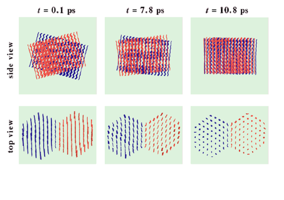
FIG. 1.: Structural evolution of two contact domains with a tilt angle $\pi/6$. Two domains are, respectively, colored by red and blue.

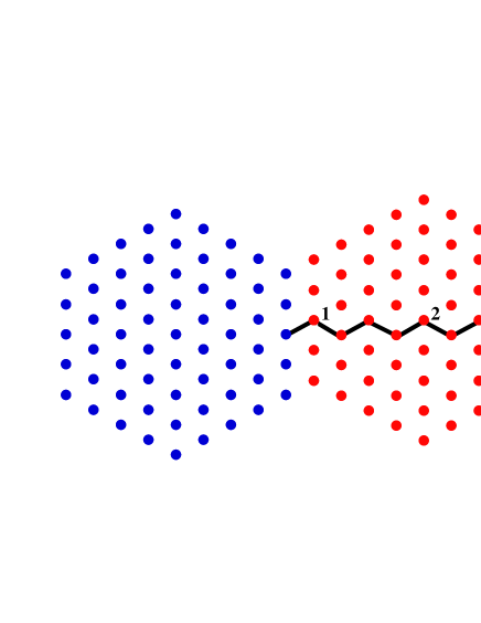
FIG. 2.: Top view of schematic configuration of (61+61) chains before tilting. A solid zigzag line denotes the shortest path of the information transfer from the contact point to the edge.

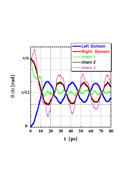
FIG. 3.: Time evolution of the angles of ${\mbox{\boldmath$U$}}^{\rm L}$ (blue), ${\mbox{\boldmath$U$}}^{\rm R}$ (red), ${\mbox{\boldmath$u$}}^{\rm R}_{1}$ (green), ${\mbox{\boldmath$u$}}^{\rm R}_{2}$ (black), and ${\mbox{\boldmath$u$}}^{\rm R}_{3}$ (purple) (Chain 1, 2 and 3 are indicated in Fig. 2).

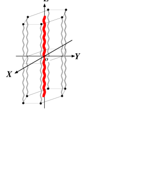
FIG. 4.: Schematic illustration of the unit hexagonal cell (7 rigid-chain model).

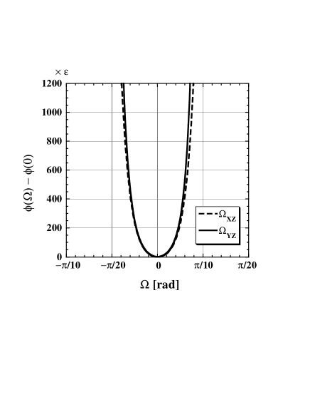
FIG. 5.: The Lennard-Jones potential of the unit hexagonal cell as a function of the rotation angle $\Omega_{i}\ \ (i=XZ,YZ)$. Rotation is made for the central rod (red) in Fig. 4 in the $XZ$ or $YZ$ plane around the origin.

REFERENCES

- [1] S. Fujiwara and T. Sato, Phys. Rev. Lett. 80, 991 (1998).
- [2] S. Fujiwara and T. Sato, Molecular Simulation 21, 271 (1999).
- [3] S. Fujiwara and T. Sato, J. Chem. Phys.110, 9757 (1999).
- [4] B. Heck, T. Hugle, M. Iijima, E. Sadiku and G. Strobl, New J. Phys. 1, 17 (1999). http://www.njp.org/
- [5] S.L. Mayo, B.D. Olafson, and W.A. Goddard III, J. Phys. Chem. 94, 8897 (1990).
- [6] W.C. Swope, H.C. Andersen, P.H. Berens and K.R. Wilson, J. Chem. Phys. 76, 637 (1982).
- [7] S. Nosé, J. Chem. Phys. 81, 511(1984).
- [8] W.G. Hoover, Phys. Rev. A 31, 1695(1985).