Quantal Andreev Billiards: Density of States Oscillations and
the Spectrum-Geometry Relationship

Abstract

Andreev billiards are finite, arbitrarily-shaped, normal-state regions, surrounded by superconductor. At energies below the superconducting energy gap, single-quasiparticle excitations are confined to the normal region and its vicinity, the mechanism for confinement being Andreev reflection. Short-wave quantal properties of these excitations, such as the connection between the density of states and the geometrical shape of the billiard, are addressed via a multiple scattering approach. It is shown that one can, inter alia, “hear” the stationary chords of Andreev billiards.

05.45.Mt, 74.80.-g, 71.24.+q

Introduction. The aim of this Letter is to explore certain quantal aspects of quasiparticle motion arising in a class of mesoscopic structures known as Andreev billiards (ABs). By the term Andreev billiard [1] we mean a connected, normal-state region (N) completely surrounded by a conventional superconducting region (S), as sketched for the 2D case in Fig. 1a. The S region is responsible for confining quasiparticles that have energies less than the superconducting energy gap to the normal region and its neighborhood [1, 2]. The terminology AB reflects the centrality of the role played by quasiparticle reflection from the surrounding pair-potential [3]. Our focus here will be on the the density of energy levels of the quasiparticle states localized near a generically shaped AB, and its relationship to the geometrical shape of the AB. The main new features that our approach is able to capture are the oscillations in the level-density caused by the spatial confinement of the quasiparticles. This structure is inaccessible via conventional quasiclassical methods.

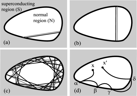
FIG. 1.: (a) Andreev billiard, showing a generic retro-reflecting orbit. (b) Orbit corresponding to a stationary chord. The length of this orbit should be contrasted with that in (c), which shows a generic “creeping” orbit due to imperfect retro-reflection; electrons (holes) follow full (shaded) lines. (d) Generic term in the multiple scattering expansion; internal (external) lines represent Green functions ${\bf G}^{\rm N}$(${\bf G}^{\rm S}$).

Our central results concern the density of states (DOS) for billiards of arbitrary shape and dimensionality. They include an explicit formula for the coarse DOS, as well as a general method for obtaining the (previously inaccessible) oscillations about this coarse DOS, both valid in the short-wave limit. This DOS decomposition is feasible because, unlike for conventional billiards, the classical trajectories of ABs fall into two well-separated classes: (i) tracings of stationary chords (see Fig. 1b), and (ii) certain extremely long trajectories with many reflections (see Fig. 1c), which contribute to the level density only at fine energy resolutions.

Our strategy for exploring the quantal properties of ABs is as follows. First, we express the Green function for the appropriate (i.e. Bogoliubov-de Gennes [4]; henceforth BdG) single-quasiparticle energy eigenproblem as an expansion in terms of various scattering processes from the N-S interface. Next, we identify which of these scattering processes dominate, by effectively integrating out processes that involve propagation inside the S region, thus arriving at an expansion involving only reflections (i.e. scattering processes that keep the quasiparticles inside the billiard). The processes associated with these reflections can be classified as those that interconvert electrons and holes (which we refer to as Andreev reflections, and which typically dominate) and those that do not (which we refer to as ordinary reflections). We then compute the oscillatory part of the DOS via two distinct asymptotic schemes.

The first scheme amounts to an elaboration of that adopted by Andreev, and is what is conventionally understood when the terms semiclassical or quasiclassical are used in the subject of superconductivity. Its physical content is perfect retro-reflection (i.e. velocity reversal) of quasiparticle excitations from the N-S boundary and perfect e/h (i.e. electron/hole) interconversion (i.e. the neglect of ordinary reflection processes). It yields a smooth (i.e. low energy-resolution) DOS, as well as singular features that arise from stationary-length chords. However, it is incapable of capturing other features in the DOS caused by the spatial confinement of quasiparticles.

The second scheme incorporates the effect of the imperfectness of retro-reflection which results from differences between, say, incident e and reflected h wave vectors, as well as the effect of ordinary reflection processes. It yields the DOS with higher energy-resolution, thus revealing the oscillations caused by spatial confinement. In order to distinguish the effect of imperfect e/h interconversion from higher-order quantum effects, we introduce and study a model that features perfect e/h interconversion but still includes all quantal effects. This model is also useful when the pair-potential varies smoothly (so that ordinary reflection is even more strongly suppressed).

Finally, for the purpose of illustration we examine the the case of a two-dimensional circular billiard, and compare the predictions for the DOS obtained via the various asymptotic schemes with those arising from the exact numerical treatment of the full BdG eigenproblem, as well as from the perfect e/h interconverting model. This provides a concrete illustration of the implications of wave phenomena for the quasiparticle quantum states of ABs.

Eigenproblem for the Andreev billiard; formulation as a boundary integral equation. To address the BdG eigenproblem for ABs we focus on the corresponding ($2\times 2$) Green function ${\bf G}$, which obeys

$$\pmatrix{-{\hat{h}}+z&{\Delta}({\bf r})\cr{\Delta}^{\ast}({\bf r})&{\hat{h}}+z\cr}{\bf G}({\bf r},{\bf r}^{\prime};z)=-{\rm I}\,\delta({\bf r}-{\bf r}^{\prime}),$$ (1)

where ${\hat{h}}\equiv-\nabla^{2}-\kappa^{2}$, together with the boundary condition that ${\bf G}$ should vanish in the limit of large $|{\bf r}|$. Here, ${\bf r}$ and ${\bf r}^{\prime}$ are spatial coordinates, $\hbar^{2}\kappa^{2}/2m$ is the Fermi energy (i.e. $\kappa$ is the Fermi wave vector), $\hbar^{2}z/2m$ is the (complex) energy, and $\hbar^{2}{\Delta}({\bf r})/2m$ is the position-dependent superconducting pair potential. The eigenfunction expansion of the Green function leads to the usual representation for the Lorentzian-smoothed DOS $\rho_{\Gamma}(E)$ of the corresponding eigenproblem:

$$\rho_{\Gamma}(E) \equiv \sum_{n}\frac{1}{\pi}\frac{\Gamma}{(E-\varepsilon_{n})^{2}+\Gamma^{2}}$$ (3)

$$= \frac{1}{\pi}\int_{{\bf r}}\lim_{{\bf r}^{\prime}\to{\bf r}}{\rm Tr}\,{\rm Im}\,{\bf G}({\bf r},{\bf r}^{\prime};E+i\Gamma),$$ (4)

where ${\rm Tr}$ denotes a trace over e/h components.

We assume that the interface between N and S is a geometrical surface constituting the boundary of the AB, i.e., is perfectly sharp. In other words, $\Delta({\bf r})$ is a constant, $\Delta_{0}$, outside the billiard and zero inside. Thus, we shall not be working self-consistently, but shall benefit from being in a position to develop an approach to the quasiparticle dynamics that focuses on interface-scattering.

To construct an expansion for the Green function ${\bf G}({\bf r},{\bf r}^{\prime};z)$ that brings to the fore the geometry of the billiard (i.e. the spatial shape of the N-S interface) we adopt the spirit of the Balian-Bloch approach to the Laplace eigenproblem [5], and construct a multiple-scattering expansion (MSE) in which the Green function is represented in terms of the fundamental N or S Green functions (i.e. those appropriate for homogeneous N or S regions). Although the physical content of this construction is intuitively clear, its development involves lengthy technical details which we defer to a forthcoming article [6]. The essence of this construction is the derivation of a system of integral equations “residing” on the N-S interface, the iterative solution of which yields the aforementioned MSE for the Green function [7]. Within this MSE approach, the amplitude for propagating from point ${\bf r}$ in N to ${\bf r}^{\prime}$ in N, viz. ${\bf G}({\bf r},{\bf r}^{\prime};z)$, is expressed as a sum of the following processes: (i) the “free” propagation amplitude ${\bf G}^{\rm N}({\bf r},{\bf r}^{\prime};z)$; (ii) the amplitude involving a single reflection [i.e. all possible amplitudes for propagating from ${\bf r}$ to a generic interface point $\textstyle\alpha$, reflecting at $\textstyle\alpha$, and then propagating to ${\bf r}^{\prime}$: $-2\int_{\alpha}\partial{\bf G}^{\rm N}({\bf r},\mathchoice{{\hbox{\boldmath$\displaystyle\alpha$}}}{{\hbox{\boldmath$\textstyle\alpha$}}}{{\hbox{\boldmath$\scriptstyle\alpha$}}}{{\hbox{\boldmath$\scriptscriptstyle\alpha$}}})\,{\mathchoice{{\hbox{\boldmath$\displaystyle\sigma$}}}{{\hbox{\boldmath$\textstyle\sigma$}}}{{\hbox{\boldmath$\scriptstyle\sigma$}}}{{\hbox{\boldmath$\scriptscriptstyle\sigma$}}}_{3}}\,{\bf G}^{\rm N}(\mathchoice{{\hbox{\boldmath$\displaystyle\alpha$}}}{{\hbox{\boldmath$\textstyle\alpha$}}}{{\hbox{\boldmath$\scriptstyle\alpha$}}}{{\hbox{\boldmath$\scriptscriptstyle\alpha$}}},{\bf r}^{\prime})$]; (iii) the amplitude involving two reflections, etc.; (iv) the amplitude that traverses the interface twice [i.e. all possible amplitudes for propagation from ${\bf r}$ to the generic interface point $\textstyle\alpha$, transmission into S, propagation in S from $\textstyle\alpha$ to another generic interface point $\textstyle\beta$, transmission into N, and propagation in N from $\textstyle\beta$ to ${\bf r}^{\prime}$: $-2^{2}\int_{\alpha}\partial{\bf G}^{\rm N}({\bf r},\mathchoice{{\hbox{\boldmath$\displaystyle\alpha$}}}{{\hbox{\boldmath$\textstyle\alpha$}}}{{\hbox{\boldmath$\scriptstyle\alpha$}}}{{\hbox{\boldmath$\scriptscriptstyle\alpha$}}})\,{\mathchoice{{\hbox{\boldmath$\displaystyle\sigma$}}}{{\hbox{\boldmath$\textstyle\sigma$}}}{{\hbox{\boldmath$\scriptstyle\sigma$}}}{{\hbox{\boldmath$\scriptscriptstyle\sigma$}}}_{3}}\,{\bf G}^{\rm S}(\mathchoice{{\hbox{\boldmath$\displaystyle\alpha$}}}{{\hbox{\boldmath$\textstyle\alpha$}}}{{\hbox{\boldmath$\scriptstyle\alpha$}}}{{\hbox{\boldmath$\scriptscriptstyle\alpha$}}},\mathchoice{{\hbox{\boldmath$\displaystyle\beta$}}}{{\hbox{\boldmath$\textstyle\beta$}}}{{\hbox{\boldmath$\scriptstyle\beta$}}}{{\hbox{\boldmath$\scriptscriptstyle\beta$}}})\,{\mathchoice{{\hbox{\boldmath$\displaystyle\sigma$}}}{{\hbox{\boldmath$\textstyle\sigma$}}}{{\hbox{\boldmath$\scriptstyle\sigma$}}}{{\hbox{\boldmath$\scriptscriptstyle\sigma$}}}_{3}}\,\delta{\bf G}^{\rm N}(\mathchoice{{\hbox{\boldmath$\displaystyle\beta$}}}{{\hbox{\boldmath$\textstyle\beta$}}}{{\hbox{\boldmath$\scriptstyle\beta$}}}{{\hbox{\boldmath$\scriptscriptstyle\beta$}}},{\bf r}^{\prime})$]; (v) and so on, where a generic term is specified by an ordered sequence of reflections and transmissions (see Fig. 1d). Here, ${\mathchoice{{\hbox{\boldmath$\displaystyle\sigma$}}}{{\hbox{\boldmath$\textstyle\sigma$}}}{{\hbox{\boldmath$\scriptstyle\sigma$}}}{{\hbox{\boldmath$\scriptscriptstyle\sigma$}}}_{1,2,3}}$ are the Pauli matrices, and the operators $\partial$ and $\delta$ are defined via

$$\partial{\bf G}({{\bf r}},{\mathchoice{{\hbox{\boldmath$\displaystyle\alpha$}}}{{\hbox{\boldmath$\textstyle\alpha$}}}{{\hbox{\boldmath$\scriptstyle\alpha$}}}{{\hbox{\boldmath$\scriptscriptstyle\alpha$}}}}) \equiv {\bf n}_{\alpha}\cdot\mathchoice{{\hbox{\boldmath$\displaystyle\nabla$}}}{{\hbox{\boldmath$\textstyle\nabla$}}}{{\hbox{\boldmath$\scriptstyle\nabla$}}}{{\hbox{\boldmath$\scriptscriptstyle\nabla$}}}_{{r}^{\prime}}{\bf G}({{\bf r}},{{\bf r}}^{\prime})|_{{{\bf r}}^{\prime}={\mathchoice{{\hbox{\boldmath$\displaystyle\alpha$}}}{{\hbox{\boldmath$\textstyle\alpha$}}}{{\hbox{\boldmath$\scriptstyle\alpha$}}}{{\hbox{\boldmath$\scriptscriptstyle\alpha$}}}}}\,,$$ (6)

$$\delta{\bf G}({\mathchoice{{\hbox{\boldmath$\displaystyle\alpha$}}}{{\hbox{\boldmath$\textstyle\alpha$}}}{{\hbox{\boldmath$\scriptstyle\alpha$}}}{{\hbox{\boldmath$\scriptscriptstyle\alpha$}}}},{{\bf r}}^{\prime}) \equiv {\bf n}_{\alpha}\cdot\mathchoice{{\hbox{\boldmath$\displaystyle\nabla$}}}{{\hbox{\boldmath$\textstyle\nabla$}}}{{\hbox{\boldmath$\scriptstyle\nabla$}}}{{\hbox{\boldmath$\scriptscriptstyle\nabla$}}}_{{r}\phantom{{}^{\prime}}}{\bf G}({{\bf r}},{{\bf r}}^{\prime})|_{{{\bf r}}\phantom{{}^{\prime}}={\mathchoice{{\hbox{\boldmath$\displaystyle\alpha$}}}{{\hbox{\boldmath$\textstyle\alpha$}}}{{\hbox{\boldmath$\scriptstyle\alpha$}}}{{\hbox{\boldmath$\scriptscriptstyle\alpha$}}}}}\,,$$ (7)

where ${\bf n}_{\alpha}$ is the normal unit vector pointing into N at $\textstyle\alpha$ on the N-S interface.

Semiclassical density of states. So far, our reformulation of the BdG eigenproblem has been exact, but many of its well-known physical features (such as the dominance of charge-interconverting reflection processes) lie hidden beneath the formalism. They will, however, emerge when we employ either of two distinct semiclassical (i.e. short-wave asymptotic) approximation schemes, as we shall shortly see. In both schemes, the DOS is calculated via Eq. (4), by using the MSE for ${\bf G}$ and evaluating the resulting integrals using the stationary-phase approximation, which is appropriate for large $\kappa L$ and small ${\Delta}/\kappa^{2}$ (where $L$ is the characteristic linear size of the AB). From the technical point of view, the difference between these schemes lies in the nature of the limits that one assumes the parameters to take: (A) $\kappa L\to\infty$ and ${\Delta}/\kappa^{2}\to 0$ with $L{\Delta}/\kappa$ constant; versus (B) $\kappa L\to\infty$ with ${\Delta}/\kappa^{2}$ constant. The limit taken determines which stationary phase points (i.e. classical reflection rules) should be applied.

In both schemes, however, it is possible to integrate out processes involving propagation inside S, to leading order in $(\kappa L)^{-1}$ and ${\Delta}/\kappa^{2}$. This is done by separating each factor of ${\bf G}^{\rm N}$ and ${\bf G}^{\rm S}$ in every kernel in the MSE into short-ranged pieces and their complements. By doing this we are distinguishing between local processes (i.e. those in which all scatterings take place within a boundary region of linear size of order $\kappa^{-1}$, so that particles ultimately leave the boundary region from a point very close to where they first reached it), and nonlocal processes (i.e. the remaining—or long-range—propagation). Then, we approximate the boundary by the tangent plane at the reflection point, and evaluate integrals involving short-ranged kernels on this plane. Moreover, contributions involving the long-ranged part of ${\bf G}^{\rm S}$ are smaller, by a factor of $(\kappa L)^{-1}$, and thus we may neglect them [8]. This procedure leads to an asymptotic expansion for ${\bf G}$, which can be used in either of the two semiclassical schemes, and which includes only interface reflection (as opposed to transmission) and, correspondingly, involves the renormalized Green function ${\bf G}^{\rm R}$:

$${\bf G}\simeq{\bf G}^{\rm N}+2\negthinspace\int_{\partial{\cal V}}\negthinspace\partial{\bf G}^{\rm N}{\bf G}^{\rm R}+2^{2}\negthinspace\int_{\partial{\cal V}}\negthinspace\partial{\bf G}^{\rm N}\,\partial{\bf G}^{\rm R}\,{\bf G}^{\rm R}+\cdots,$$ (8)

$${\bf G}^{\rm R}\equiv\Big{(}-i{\rm e}^{-i\varphi}{\mathchoice{{\hbox{\boldmath$\displaystyle\sigma$}}}{{\hbox{\boldmath$\textstyle\sigma$}}}{{\hbox{\boldmath$\scriptstyle\sigma$}}}{{\hbox{\boldmath$\scriptscriptstyle\sigma$}}}_{1}}+{\cal O}\left((\kappa L)^{-2},{\Delta}/\kappa^{2}\right)\Big{)}\,\,{\bf G}^{\rm N},$$ (9)

$${\bf G}^{\rm N}({\bf r},{\bf r}^{\prime})\equiv\pmatrix{g_{+}({\bf r}-{\bf r}^{\prime})&0\cr 0&-g_{-}({\bf r}-{\bf r}^{\prime})},$$ (10)

where $\varphi\equiv\cos^{-1}(E/{\Delta})$, $g_{\pm}({\bf r})\equiv H_{0}^{\pm}\big{(}k_{\pm}|{{\bf r}}|\big{)}/4$ in two dimensions and $g_{\pm}({\bf r})\equiv\exp\left(\pm ik_{\pm}|{{\bf r}}|\right)/{4\pi|{{\bf r}}|}$ in three dimensions, $k_{\pm}=\sqrt{\kappa^{2}\pm E}$ are the e/h wave vectors, the integrals are taken over the the interface $\partial{\cal V}$, and, e.g., $\int_{\partial{\cal V}}\partial{\bf G}^{\rm N}{\bf G}^{\rm R}\equiv\int_{\partial{\cal V}}d\mathchoice{{\hbox{\boldmath$\displaystyle\alpha$}}}{{\hbox{\boldmath$\textstyle\alpha$}}}{{\hbox{\boldmath$\scriptstyle\alpha$}}}{{\hbox{\boldmath$\scriptscriptstyle\alpha$}}}\partial{\bf G}^{\rm N}({\bf r},\mathchoice{{\hbox{\boldmath$\displaystyle\alpha$}}}{{\hbox{\boldmath$\textstyle\alpha$}}}{{\hbox{\boldmath$\scriptstyle\alpha$}}}{{\hbox{\boldmath$\scriptscriptstyle\alpha$}}})\,{\bf G}^{\rm R}(\mathchoice{{\hbox{\boldmath$\displaystyle\alpha$}}}{{\hbox{\boldmath$\textstyle\alpha$}}}{{\hbox{\boldmath$\scriptstyle\alpha$}}}{{\hbox{\boldmath$\scriptscriptstyle\alpha$}}},{\bf r}^{\prime})$. Observe that the leading term in ${\bf G}^{\rm R}$ includes only charge-interconverting processes; ordinary reflection appears only at sub-leading order. In physical terms, the approximation that we have invoked takes into account the fact that an electron wave incident on an N-S interface “leaks” into the S side and, consequently, is partially converted into a hole and acquires a phase, much as a particle acquires a phase (i.e. a Maslov index) when reflected by a finite single-particle potential.

We are now in a position to define what we shall call the Perfectly Charge-Interconverting Model (PCIM). We start with the expansion (10) for ${\bf G}$ in terms of ${\bf G}^{\rm R}$, and take the latter to be given by its leading-order form: ${\bf G}^{\rm R}\approx-i{\rm e}^{-i\varphi}{\mathchoice{{\hbox{\boldmath$\displaystyle\sigma$}}}{{\hbox{\boldmath$\textstyle\sigma$}}}{{\hbox{\boldmath$\scriptstyle\sigma$}}}{{\hbox{\boldmath$\scriptscriptstyle\sigma$}}}_{1}}{\bf G}^{\rm N}$. Then the PCIM is defined via the following integral equation for ${\bf G}$:

$${\bf G}={\bf G}^{\rm N}-2i{\rm e}^{-i\varphi}\negthinspace\int_{\partial{\cal V}}\negthinspace\partial{\bf G}^{\rm N}{\mathchoice{{\hbox{\boldmath$\displaystyle\sigma$}}}{{\hbox{\boldmath$\textstyle\sigma$}}}{{\hbox{\boldmath$\scriptstyle\sigma$}}}{{\hbox{\boldmath$\scriptscriptstyle\sigma$}}}_{1}}{\bf G}\,.$$ (11)

The off-diagonal matrix ${\mathchoice{{\hbox{\boldmath$\displaystyle\sigma$}}}{{\hbox{\boldmath$\textstyle\sigma$}}}{{\hbox{\boldmath$\scriptstyle\sigma$}}}{{\hbox{\boldmath$\scriptscriptstyle\sigma$}}}_{1}}$ ensures that, upon each reflection from the boundary, electrons are fully converted into holes (and vice versa). Moreover, this model does retain wave propagation effects, as implied by the surface integral.

Let us now focus on semiclassical Scheme A, which is, in spirit, the one introduced by Andreev [3]. In this scheme, excitations undergo perfect retro-reflection (i.e. perfect velocity-reversal), as well as perfect charge-interconversion, so that the dynamics is confined to the geometrical chords of the AB and, thus, is trivially integrable, whatever the shape of the AB [1]. Via this scheme, we arrive at the following form for the DOS:

$\displaystyle\rho_{\Gamma}(E)\simeq\int_{\partial{\cal V}}\negthinspace\negthinspace{\rm Re}\,\,{\cos\theta_{\alpha\beta}\,\cos\theta_{\beta\alpha}\over{1-\exp\left[{i(E/\kappa)|{\mathchoice{{\hbox{\boldmath$\displaystyle\alpha$}}}{{\hbox{\boldmath$\textstyle\alpha$}}}{{\hbox{\boldmath$\scriptstyle\alpha$}}}{{\hbox{\boldmath$\scriptscriptstyle\alpha$}}}}-{\mathchoice{{\hbox{\boldmath$\displaystyle\beta$}}}{{\hbox{\boldmath$\textstyle\beta$}}}{{\hbox{\boldmath$\scriptstyle\beta$}}}{{\hbox{\boldmath$\scriptscriptstyle\beta$}}}}|-2i\varphi}\right]}}\Big{|}_{E\to E+i\Gamma}.$

Here, the integral is taken over the surface points $\textstyle\alpha$ and $\textstyle\beta$, and $\theta_{\alpha\beta}$ denotes the angle between the normal at $\textstyle\alpha$ and the chord leading to $\textstyle\beta$. This equation for $\rho_{\Gamma}$ can be understood as follows: a chord of length $|{\mathchoice{{\hbox{\boldmath$\displaystyle\alpha$}}}{{\hbox{\boldmath$\textstyle\alpha$}}}{{\hbox{\boldmath$\scriptstyle\alpha$}}}{{\hbox{\boldmath$\scriptscriptstyle\alpha$}}}}-{\mathchoice{{\hbox{\boldmath$\displaystyle\beta$}}}{{\hbox{\boldmath$\textstyle\beta$}}}{{\hbox{\boldmath$\scriptstyle\beta$}}}{{\hbox{\boldmath$\scriptscriptstyle\beta$}}}}|$ contributes eigenvalue weight at energies given by the well-known semiclassical quantization condition $E\kappa^{-1}|{\mathchoice{{\hbox{\boldmath$\displaystyle\alpha$}}}{{\hbox{\boldmath$\textstyle\alpha$}}}{{\hbox{\boldmath$\scriptstyle\alpha$}}}{{\hbox{\boldmath$\scriptscriptstyle\alpha$}}}}-{\mathchoice{{\hbox{\boldmath$\displaystyle\beta$}}}{{\hbox{\boldmath$\textstyle\beta$}}}{{\hbox{\boldmath$\scriptstyle\beta$}}}{{\hbox{\boldmath$\scriptscriptstyle\beta$}}}}|-2\cos^{-1}(E/{\Delta})=2n\pi$ (for $n$ integral). However, in order to obtain $\rho_{\Gamma}$ we must sum over all chords with the proper weighting, which is accomplished by the double integral in over the boundary. The most prominent features emerging this Scheme A expression for $\rho_{\Gamma}$ are singularities, representing the strong bunching of exact eigenenergies at energies corresponding to stationary-length chords. (Such chords have both ends perpendicular to the billiard boundary.)  However, to sum over all chords would be superfluous, as the strongest features in the DOS can be captured simply from the neighborhoods of the stationary chords. Moreover, for finite values of the parameters (i.e. $\kappa L$ large but not infinite, and ${\Delta}/\kappa^{2}$ small but non-vanishing) Scheme A produces a locally averaged DOS, which becomes numerically accurate only around the DOS singularities that it predicts. Thus, it fails to capture this DOS oscillations due to the confinement of the quasiparticles. The reason for this failure is the fact that by summing over all chords one is implicitly assuming the absence of transverse quantization/confinement. To capture such oscillations is the main motivation for semiclassical Scheme B.

In Scheme B we first take into account the imperfectness in retro-reflection arising from the the previously-neglected difference between the wave vectors of incident and reflected electrons and holes, whilst neglecting all amplitudes involving ordinary reflection. The corresponding classical dynamics is no longer a priori integrable; on the contrary, it is chaotic for generic shapes [1]. In this scheme, the closed periodic orbits fall into two classes, quite distinct from one another: one consists of multiple tracings of each stationary chord (we refer to such chords as $\Lambda$s); the other of much longer trajectories that “creep” around the billiard boundary (see Fig. 1c). Correspondingly, the DOS is the sum of (i) an average term $\rho_{\rm av}(E)$, which depends in 3D on the volume (or in 2D on the area) of the billiard (i.e. the leading Weyl term); together with an oscillatory term $\rho_{\rm osc}(E)$ consisting of (ii) a finer-resolution term, having a universal line-shape that depends solely on the length and endpoint-curvatures of the $\Lambda$s [9], and (iii) very fine resolution terms, which depend on the classical dynamics of the billiard in question:

$$\rho_{\rm osc}(E) \simeq {\rm Re}\!\sum_{\ell_{{\Lambda}}}\!Z_{{\Lambda}}\,{\rm e}^{i\lambda_{{\Lambda}}\pi/4}{\rm Li}_{d-1-\frac{w}{2}}(1\!-\!{\rm e}^{i(k_{+}-k_{-})\ell_{{\Lambda}}-2i\varphi})$$ (12)

$$+ \sum_{\rm periodic\ orbits}A_{\rm po}\,\exp{iS_{\rm po}}\,\,.$$ (13)

Here, ${\rm Li}_{n}(z)\equiv\sum_{j=1}^{\infty}z^{j}/j^{n}$ is the polylogarithm function, $d$ is the dimensionality of the billiard, $w$ is the dimensionality of the degeneracy of the $\Lambda$ (e.g. $w=1$ for a circle), $Z_{{\Lambda}}$ is a slowly-varying real function of energy, determining the size of the DOS oscillations, and $\lambda_{{\Lambda}}$ is a measure of the stability of the $\Lambda$, which determines whether the “tail” goes towards higher or lower energies. For example, an isolated $\Lambda$ in 2D would yield $\lambda_{{\Lambda}}={\rm sgn}(R_{1}+R_{2}-\ell_{{\Lambda}})-1$ and

$$Z_{{\Lambda}}=\sqrt{\frac{(k_{+}+k_{-})^{2}\ell_{{\Lambda}}R_{1}R_{2}}{4\pi^{2}k_{+}k_{-}(k_{+}-k_{-})^{2}|\ell_{{\Lambda}}-R_{1}-R_{2}|}},$$ (14)

where $R_{1}$ and $R_{2}$ are the radii of curvature of the endpoints of the $\Lambda$ [10]. The second term in Eq. (13) is the contribution from “creeping” orbits (see Fig. 1c). In it, $A_{\rm po}$ is determined by the stability of the orbit, and $S_{\rm po}$ is the action corresponding to the orbit. For a typical AB, $S_{\rm po}>N\big{(}(k_{+}-k_{-})\ell_{{\Lambda}}-2\varphi\big{)}$, where $N={\cal O}(\kappa^{2}/{\Delta})$ and, thus, “creeping” orbits contribute only to the very fine details of the DOS.

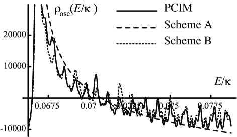
FIG. 2.: Density of states oscillations for a circular AB: $\kappa R=150$; ${\Delta}/\kappa^{2}=0.08$; smoothing width $\Gamma/\kappa^{2}=1.1\times 10^{-4}$.

For illustration, in Fig. 2 we compare the predictions of Schemes A and B with those of the PCIM. The Scheme-A result (dashed line) approximates the average behavior of the exact DOS for the PCIM (full line). In contrast, the Scheme-B result (dotted line) captures the DOS oscillations arising from transverse quantization/confinement.

Thus far in our semiclassical treatment, we have ignored all amplitudes involving ordinary reflection. For non-grazing incidence [i.e. $\theta-(\pi/2)\sim 1$] the amplitude for ordinary reflection is very small ($\sim{\Delta}/\kappa^{2}\cos^{2}\theta)$). However, for orbits that contribute dominantly to the oscillatory structure of the DOS, $|\theta-(\pi/2)|\ll 1$ and, therefore, ordinary reflection amplitudes are not negligible and must be incorporated. This can be done by returning to Eq. (10) and re-evaluating the trace formula using the full expression for ${\bf G}^{\rm R}$ (i.e. not just the leading, off-diagonal, term). However, these dominating orbits are the ones that are close to the boundary and, for these, consecutive reflections take place very near to each other, and thus “see” only the local curvature of the boundary. These considerations allow us to perform an “adiabatic” approximation to the expansion in Eq. (10), in which we assume that the curvature of the boundary varies slowly, relative to the rate at which creeping orbits sample the boundary. In Fig. 3 we compare this adiabatic method with the (exact) result obtained by solving the full BdG eigenproblem.

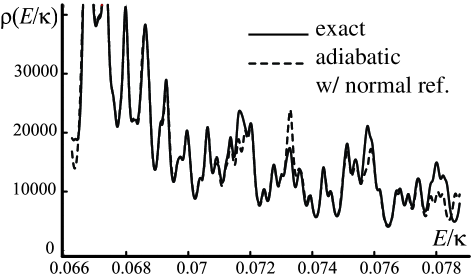
FIG. 3.: Density of states for a circular AB: $\kappa R=150$; ${\Delta}/\kappa^{2}=0.08$; smoothing width $\Gamma/\kappa^{2}=1.1\times 10^{-4}$.

We conclude by emphasizing one particular feature of the first term in Eq. (13): this term gives the coarse DOS directly, through simple geometrical information in the form of the lengths and endpoint-curvatures of the $\Lambda$s. This feature allows the design of an AB shape that leads to a DOS having a predetermined coarse form. Moreover, as the stationary-chord terms are well separated (in time-space) from the creeping orbits, it possible to “hear” not only the volume of an Andreev billiard but also its stationary chords.

Acknowledgments. We gratefully acknowledge useful discussions with Eric Akkermanns, Michael Stone and especially Dmitrii Maslov. This work was supported by DOE DEFG02-96ER45439 and NSF-DMR-99-75187.

REFERENCES

- [1] Certain classical properties of ABs were discussed in I. Kosztin, D. L. Maslov and P. M. Goldbart, Phys. Rev. Lett. 75 1735 (1995).
- [2] Certain quantum mechanical properties of ABs were studied in A. Altland and M. R. Zirnbauer, Phys. Rev. Lett. 76, 3420 (1996); K. M. Frahm et al., Phys. Rev. Lett. 76, 2981 (1996); J. A. Melsen et al., Europhys. Lett. 35, 7 (1996); Physica Scripta T 69, 223 (1997); A. Lodder and Yu. V. Nazarov, Phys. Rev. B 58, 5783 (1998); H. Schomerus and C. W. J. Beenakker, Phys. Rev. Lett. 82, 2951 (1999); W. Ihra et al., cond-mat/9909100.
- [3] A. F. Andreev, Zh. Eksp. Teor. Fiz. 46, 1823 (1964) [Sov. Phys. J.E.T.P. 19, 1228 (1964)].
- [4] See, e.g., P.-G. de Gennes, Superconductivity of metals and alloys (Addison-Wesley, New York, 1966), Chap. 5.
- [5] R. Balian and C. Bloch, Ann. Phys. (NY) 60, 401 (1970); ibid. 84, 559(E) (1974); ibid. 69, 76 (1972).
- [6] İ. Adagideli and P. M. Goldbart, in preparation (2001).
- [7] For an introduction to boundary integral equation techniques, see, e.g., R. B. Guenther and J. W. Lee, Partial differential equations of mathematical physics and integral equations, (New York: Dover, 1996), Sec. 8-7.
- [8] In fact, for concave shapes there will be nonlocal modifications that account for tunneling effects.
- [9] For isolated stationary chords this term has corrections due to changes in stability that occur when the number of reflections is very large.
- [10] The apparent singularity at is an artifact of the assumption of imperfectness in retro-reflection; this imperfectness ceases at .