[

Point-Contact Conductances from Density Correlations

Abstract

We formulate and prove an exact relation which expresses the moments of the two-point conductance for an open disordered electron system in terms of certain density correlators of the corresponding closed system. As an application of the relation, we demonstrate that the typical two-point conductance for the Chalker-Coddington model at criticality transforms like a two-point function in conformal field theory.

]

In mesoscopic physics, as well as in quantum physics at large, open systems are distinguished from closed ones. The difference is most evident from the nature of the corresponding energy spectra: when a closed and finite system is opened up, the discrete set of stationary solutions of the Schrödinger equation turns into a continuum. In the open case, one usually looks for solutions in the form of scattering states, where the wave amplitudes are prescribed in all incoming channels and the outgoing waves are then related to the incoming ones by a linear operator called the scattering matrix or $S$-matrix.

One may ask whether one can connect the scattering matrix of an open system with the properties of its closed analog. In spite of the physical distinction between open and closed systems, such connections do exist. For example, for noninteracting quasi-one-dimensional electrons subject to weak disorder it has been found [1] that the parametric correlations between the eigenphases of the $S$-matrix exhibit behavior similar to that of the energy levels of the closed system. For another example, the $S$-matrix (or rather its extension including evanescent modes) has been utilized [2] in numerical algorithms that compute large numbers of energy eigenvalues for a chaotic closed billiard. An intimately related scheme is provided by Bogomolny’s semiclassical T-operator [3].

All these theoretical developments were primarily concerned with the energy levels and their statistics. In the present Letter we address a different question: suppose a closed system has been opened, what relations, if any, exist between the statistical properties of the $S$-matrix and the stationary wavefunctions of the closed system? This question is of practical relevance, as the $S$-matrix determines the electrical conductance of an open mesoscopic device. It will be seen that, provided a few well-formulated conditions are satisfied, an informative answer can be given. While this seems unlikely if the system is perturbed strongly, say by making the boundaries transparent, the situation is different if one uses point contacts which establish the connection to the outside through ideal one-dimensional channels. For concreteness and simplicity, we are going to develop the theory for the case where time is a discrete variable, but we anticipate that a variant of the relation to be derived remains valid for systems with continuous-time dynamics generated by a Hamiltonian.

We begin by briefly reviewing the concept of network models. Wave or quantum-particle propagation in a random medium or a chaotic cavity can be modeled by a network (or graph) consisting of internal channels represented by links and of local scattering centers represented by nodes. For a network with $N$ links, the state is specified by $N$ complex amplitudes that assemble into a vector $\Psi=\{\psi_{l}\}_{l=1,\cdots,N}$. The network evolves in time by repeated application of a unitary matrix $U\in{\rm U}(N)$, which propagates states between integer times $t$: $\Psi(t+1)=U\Psi(t)$. Stationary states $\Psi_{j}=\{\psi_{j,l}\}$ and quasi-energy levels $0\leq\omega_{1}\leq\dots\leq\omega_{N}<2\pi$ are constructed by solving the eigenvalue problem $U\Psi_{j}={\rm e}^{i\omega_{j}}\Psi_{j}$. By the local intensity $\rho_{j,l}$ of $\Psi_{j}$ we mean the squared amplitude $|\psi_{j,l}|^{2}$ of the normalized state $\Psi_{j}$ at link $l$.

The previous definitions apply for closed networks, where each link starts and ends at a network node. To define a conductance, however, one needs to connect the network to external charge reservoirs. We do this by introducing two interior point contacts, i.e. by cutting the network open at two links $l$ and $m$, thereby producing two incoming and outgoing channels. If we imagine these channels to be connected to Ohmic contacts, the upshot of the surgery done on the network is to define a two-terminal conductance between the points $l$ and $m$. We denote it by $T_{lm}$ and refer to it as the two-point conductance for short. The inset of Fig. 1 shows the basic setup at the example of the Chalker-Coddington network [4].

Given the $2\times 2$ scattering matrix $S={\pmatrix{S_{ll}&S_{lm}\cr S_{ml}&S_{mm}\cr}}$ which consists of the amplitudes for transmission and reflection by the open network, the Landauer-Büttiker formula states that $T_{lm}$ (at zero temperature, and in units of the conductance quantum $e^{2}/h$) equals the transmission probability $|S_{lm}|^{2}$. For the following it will be crucial that $S$, though primarily defined for the open network, can also be expressed [5] entirely in terms of the unitary time-evolution operator $U$ of the closed system:

$$S_{\alpha\beta}=\left\langle\alpha\left|(1-UP_{l}P_{m})^{-1}U\right|\beta\right\rangle\quad(\alpha,\beta=l,m)$$ (1)

where $P_{k}=1-|k\rangle\langle k|$. Expansion of $(1-UP_{l}P_{m})^{-1}$ in a geometric series shows that $S_{\alpha\beta}$ is a sum over path amplitudes for paths from $\beta$ to $\alpha$. The projection operators $P_{l}$ and $P_{m}$ serve to truncate paths as soon as they arrive at the outgoing channel of either terminal $l$ or $m$.

Via relation (1), every disorder average ${\left\langle\cdots\right\rangle}$ of the closed system determines a disorder average pertaining to the $S$-matrix of the open system. In particular, the average of any function of the two-point conductance is defined, by ${\left\langle F(T_{lm})\right\rangle}\equiv{\left\langle F\left(\big{|}\langle l|(1-UP_{l}P_{m})^{-1}U|m\rangle\big{|}^{2}\right)\right\rangle}$.

Starting from some disordered network model, our aim in the sequel is to relate the distribution of two-point conductances to the statistics of stationary wavefunctions. As will be seen, the relation we are going to derive does not depend on the details of the model chosen. The only requirements we need are two conditions constraining the disorder average: the phases of the reflection coefficients $S_{ll}$ and $S_{mm}$ must be (i) uniformly distributed and independent of each other, and (ii) statistically independent of $T_{lm}$. These conditions are automatically satisfied for the Chalker-Coddington model and more generally for all models with local phase invariance.

Given some choice of model with disorder average ${\left\langle\cdots\right\rangle}$, we introduce an additional average ${\left\langle\cdots\right\rangle}_{{\rm e}}$ for observables that can be expressed by the stationary states $\Psi_{j}$:

$${\left\langle A\right\rangle}_{{\rm e}}:=\frac{1}{\varepsilon\nu}\int_{0}^{\varepsilon}d\omega\sum_{j=1}^{N}\left\langle\delta(\omega-\omega_{j})A(\Psi_{j})\right\rangle\;,$$ (2)

where $\nu$ is the level density at $\omega=0$, and $\varepsilon$ sets the size of an energy window. In what follows, we take $\varepsilon\to 0$, restricting the sum over states to the first level, $\omega_{1}$.

We are now in a position to propose a statistical relation between $T_{lm}$ and the intensities $\rho_{l}=|\psi_{1,l}|^{2}$ and $\rho_{m}=|\psi_{1,m}|^{2}$. Let $f(x)$ be any function defined for $x$ in the positive real numbers. Then we claim [6]

$$2\pi\nu\>{\left\langle\rho_{m}f\left({\rho_{m}}/{\rho_{l}}\right)\right\rangle}_{{\rm e}}={\left\langle F(T_{lm})\right\rangle}\>,\quad{\rm where}$$ (3)

$$F(T):=\int_{0}^{2\pi}\frac{d\varphi}{2\pi}\>f\left(T^{-1}|1-{\rm e}^{i\varphi}\sqrt{1-T}|^{2}\right)\>.$$ (4)

A first remark on (3) is that, in view of the scaling $\nu\sim N$ and $\rho_{m}\sim N^{-1}$ (on average over the statistical ensemble), the system size $L^{d}\sim N$ drops out of the combination $\nu\rho_{m}f(\rho_{m}/\rho_{l})$, reflecting the fact [7] that $T_{lm}$ tends to a finite limit as $L$ is sent to infinity. Note that the plain correlator $\nu^{2}{\left\langle\rho_{l}\rho_{m}\right\rangle}$ does not share [8] this property of size independence, which is why any attempt to express it through such relations as (3-4) is met with failure.

More explicit relations are obtained by adopting special choices for $f$. Of particular interest is an expression giving the typical conductance $T_{lm}^{\rm typ}\equiv\exp{\left\langle\ln T_{lm}\right\rangle}$:

$${\left\langle\ln T_{lm}\right\rangle}=2\pi\nu\>{\left\langle\rho_{m}\ln(\rho_{l}/\rho_{m})\right\rangle}_{{\rm e}}\>,$$ (5)

which follows from (3-4) on taking $f(x)=-\ln x$. Another simple relation results on setting $f(x)=(1+x)^{-1}$:

$$\langle\sqrt{T_{lm}}\rangle=4\pi\nu\>{\left\langle\rho_{l}\rho_{m}/(\rho_{l}+\rho_{m})\right\rangle}_{{\rm e}}\>.$$

Furthermore, by inverting the relation gotten by setting $f(x)=x^{n}$, and analytically continuing from integer $n$ to complex $z$, it can be shown with some effort that

$${\left\langle T_{lm}^{z}\right\rangle}=\sum_{k=0}^{\infty}\frac{(2k+1)\>\Gamma(1-z)^{2}\>2\pi\nu}{\Gamma(k+2-z)\Gamma(1-k-z)}{\left\langle\rho_{m}^{k+1}\rho_{l}^{-k}\right\rangle}_{{\rm e}}\>.$$

Note that the sum over $k$ is terminated by the poles of the gamma function when $z$ is a negative integer or zero. For all other values of $z$, the series will in general be divergent, since the polynomial decay of the product of inverse gamma functions does not suffice to control the growth with $k$ of the moments $\langle\rho_{m}^{k+1}\rho_{l}^{-k}\rangle$. Fortunately, if $z=n+1/2$ with $n$ a positive integer, the series can be rearranged to produce a finite sum involving polynomials in the bounded random variable $\rho_{l}\rho_{m}/(\rho_{l}+\rho_{m})^{2}\leq 1/4$:

$$\langle T_{lm}^{n+1/2}\rangle={\left({2n}\atop{n}\right)}^{-1}\sum_{k=0}^{n}\left({2k}\atop{k}\right){\mu_{n-k}\over 1-2k}\;,$$ (6)

where $\mu_{n}=2^{4n+2}\pi\nu{\left\langle(\rho_{l}\rho_{m})^{n+1}(\rho_{l}+\rho_{m})^{-2n-1}\right\rangle}_{{\rm e}}$. We will put this formula to good use below.

Our main result is relation (3). Its proof is based on the observation that for a network at resonance, i.e. for $\omega_{1}=0$, the corresponding eigenvector $\Psi_{1}$ of $U$ can be interpreted as a scattering state of the network opened at the links $l$ and $m$. In other words, the two amplitudes $\psi_{1,l}$ and $\psi_{1,m}$ of an eigenstate $\Psi_{1}=U\Psi_{1}$ constitute at the same time an eigenvector $(\psi_{1,l},\psi_{1,m})$ with eigenvalue unity of the scattering matrix $S$. Thus we have $S_{ll}\psi_{1,l}+S_{lm}\psi_{1,m}=\psi_{1,l}$ and therefore, assuming $\psi_{1,l}S_{lm}\neq 0$,

$$\frac{\rho_{m}}{\rho_{l}}=\frac{|1-S_{ll}|^{2}}{|S_{lm}|^{2}}=\frac{|1-{\rm e}^{i\arg{S_{ll}}}\sqrt{1-T_{lm}}|^{2}}{T_{lm}}\;.$$ (7)

The next step will be to take the disorder average of this equation, viewing both sides as functions on the closed network. Of course, since (7) holds only for networks at resonance, it is imperative that we restrict the disorder average to the resonant realizations. We do this by tuning the random phase $\varphi_{m}$ at link $m$ to a function $\varphi_{m}=\varphi_{m}^{0}(\xi)$ of all other random variables $\xi=\{\xi_{1},\xi_{2},...\}$ so that $\omega_{1}(\xi,\varphi_{m}^{0}(\xi))=0$ is identically satisfied for all $\xi$ [9]. The restricted or resonant disorder average thus defined is denoted by ${\left\langle\cdots\right\rangle}_{{\rm res},m}$. By applying some function $f$ to the identity (7) and averaging in this manner we get

$$\left\langle f\left(\frac{\rho_{m}}{\rho_{l}}\right)\right\rangle_{{\rm res},m}={\left\langle f\left(\frac{|1-{\rm e}^{i\varphi_{l}}\sqrt{1-T_{lm}}|^{2}}{T_{lm}}\right)\right\rangle}_{{\rm res},m},$$

where we have set $\varphi_{l}\equiv\arg{S_{ll}}$. Now recall that, according to conditions (i) and (ii), the phase $\varphi_{l}$ is statistically independent of $\varphi_{m}$ and $T_{lm}$ and is uniformly distributed. Consequently, the preceding equation continues to hold if we integrate the r.h.s. with measure $d\varphi_{l}/2\pi$ over $[0,2\pi]$, thereby turning it into ${\left\langle F(T_{lm})\right\rangle}_{{\rm res},m}$ with $F$ defined by (4). Moreover, condition (ii) entails that the resonant average ${\left\langle F(T_{lm})\right\rangle}_{{\rm res},m}$ actually equals the natural average ${\left\langle F(T_{lm})\right\rangle}$. Thus

$${\left\langle f(\rho_{m}/\rho_{l})\right\rangle}_{{\rm res},m}={\left\langle F(T_{lm})\right\rangle}\>.$$ (8)

Next we transform the average over resonant networks on the l.h.s. to the eigenfunction average (2), as follows:

$$2\pi\nu\>{\left\langle A\right\rangle}_{{\rm e}}=\lim_{\varepsilon\to 0}\frac{2\pi}{\varepsilon}\int_{0}^{\varepsilon}d\omega\>{\left\langle\delta(\omega_{1}-\omega)A(\Psi_{1})\right\rangle}=$$

$$\int\limits_{0}^{2\pi}d\varphi_{m}\>{\left\langle\delta\big{(}\omega_{1}(\xi,\varphi_{m})\big{)}A(\Psi_{1})\right\rangle}_{\xi}={\left\langle{A(\Psi_{1})\over|\partial\omega_{1}/\partial\varphi_{m}|}\right\rangle}_{{\rm res},m}.$$

Setting $A=\left|{\partial\omega_{1}\over\partial\varphi_{m}}\right|f(\rho_{m}/\rho_{l})$ and using (8) we arrive at

$${\left\langle F(T_{lm})\right\rangle}=2\pi\nu\>{\left\langle\left|\frac{\partial\omega_{1}}{\partial\varphi_{m}}\right|f{\left(\frac{\rho_{m}}{\rho_{l}}\right)}\right\rangle}_{{\rm e}}\>.$$

Finally, since a phase variation $\delta\varphi_{m}$ perturbs the time-evolution operator $U$ by $i(\delta\varphi_{m})|m\rangle\langle m|U$, standard first-order perturbation theory shows that the level velocity $|\partial\omega_{1}/\partial\varphi_{m}|$ equals $\rho_{m}$. This concludes the proof.

It is easily seen that the above line of reasoning does not depend in any essential way on assuming a network model with discrete time. In fact, a slight variant of the argument goes through for continuous-time dynamics generated by a Hamiltonian $H$. What one needs to do is attach two identical and strictly one-dimensional leads $l$ and $m$ to the system, which are then either connected to charge reservoirs, or else closed off by imposing reflecting boundary conditions at variable lengths $L_{l}$ and $L_{m}$. The intensity $\rho_{l(m)}$ of the closed system is interpreted as $\int_{x_{0}}^{x_{0}+\lambda}dx\;|\psi(x)|^{2}$ where $\lambda$ is the wavelength and $x_{0},x_{0}+\lambda$ are in the closed lead $l(m)$. The normalization factor $2\pi\nu$ in Eq. (3) has to be replaced by ${\left\langle\rho_{m}\right\rangle}^{-1}$. To tune the system to a given resonance energy $E$, we adjust $L_{m}$.

At the moment it is not clear to us to which extent, if at all, the relation applies to systems with more than two point contacts or more general types of contact. This point deserves further investigation.

When states are localized, relation (5) implies that the decay length of the typical two-point conductance agrees with the typical localization length of the states of the closed system. While this has long been known for strictly one-dimensional systems [10], it is now seen to hold exactly under the much more general conditions we have specified. By word of caution, however, we recall that our formula does not cover correlators like $\nu^{2}\langle\rho_{l}\rho_{m}\rangle$, so it does not settle a recent debate as to whether two-scale localization in a magnetic field can occur [11] for closed systems when it does not [12] for open ones.

We now demonstrate the utility of the result (3) by applying it to a challenging problem: critical transport at the integer quantum Hall (IQH) transition [13]. To make analytical progress with that transition, one needs to confront the question what can be learned from conformal field theory. For critical systems without disorder, the principle of conformal invariance has proven to be very powerful, by posing strong constraints on correlation functions and determining how they transform between various geometries [14]. The question whether the same principle applies to 2d disordered critical points was first raised by Chalker [15]. The answer turned out to be negative for the correlation functions he considered. However, as we now proceed to demonstrate, conformal invariance does govern the two-point conductances.

An analytical formula for the distribution of two-point conductances $T\equiv T_{lm}$ for critical quantum Hall systems in the infinite plane was proposed in [5]. Given that formula, conformal field theory predicts the probability measure $d\mu(T)$ for the conductance between two points with coordinates $(0,0)$ and $(x,y)$ on an infinitely long cylinder of circumference $W$ to be given by

$$d\mu(T) = p(T^{-1}-1)T^{-2}dT\;,$$ (9)

$$p(\rho) = {2\pi^{-1/2}\ \zeta^{-X_{\rm t}/4}\over(X_{\rm t}\ln\zeta)^{3/2}}\int\limits_{{\rm arsinh}\sqrt{\rho}}^{\infty}{{\rm e}^{-t^{2}/(X_{\rm t}\ln\zeta)}tdt\over\sqrt{\sinh^{2}t-\rho}}\;,$$ (10)

$$\zeta = (W/\pi a)\left|\sinh\big{(}\pi(x+iy)/W\big{)}\right|\>,$$ (11)

where $X_{\rm t}$ is a critical exponent (unknown as yet from theory), and $a$ is a nonuniversal microscopic scale that sets the length unit in which to express the correlation functions of the particular IQH model considered.

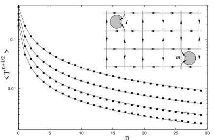
FIG. 1.: Half-integer moments ${\left\langle T^{n+1/2}\right\rangle}$ for $n=0,\dots,29$ of the two-point conductance of the Chalker-Coddington model at criticality. The four data sets correspond to contact distances $x=5,10,15$ and 20 (top to bottom) in a cylinder geometry with length $L=100$ and circumference $W=10$. Solid lines represent the theoretical prediction. Inset: Chalker-Coddington network connected to external charge reservoirs via two interior point contacts.

To test this prediction, we numerically calculated the eigenfunctions of the critical time-evolution operator $U$ of the Chalker-Coddington model, in a cylindrical geometry with large aspect ratios $L/W$, $100\leq L\leq 200$ and $3\leq W\leq 30$. An ensemble of 5000 disorder realizations was employed. Using Eq. (6) we computed the moments $\langle T^{n+1/2}\rangle$ by averaging over the pairs of links $(l,m)$ with a given distance $|x|$ and their difference vector pointing along the axis of the cylinder. The great advantage of this indirect approach (in contradistinction with the direct method of [5]) is that a large number $\sim N^{2}$ of data points can be extracted from a single eigenfunction $\Psi$. Since the numerical effort of calculating $\Psi$ and $T_{lm}$ is comparable, we gain in efficiency by a factor $N^{2}\sim(LW)^{2}$, which can be many orders of magnitude.

In Fig. 1 theory and numerics are compared for $W=10$, $L=100$, and $|x|=5,10,15,20$ (in plaquette units). The theoretical curves were obtained by numerically integrating (9) against $T^{n+1/2}$. We find that an exponent $X_{\rm t}=0.54\pm 0.01$ (and $a=0.20$) yields the best fit. The statistical errors are estimated to be comparable with the symbol size. The agreement is clearly very good, showing that the result predicted by conformal field theory interpolates correctly between 2d behavior at short distances and quasi-1d behavior at large scales.

The most clear-cut test of conformal invariance is offered by the typical two-point conductance. By integrating (9) against $\ln T$, one finds a very simple law [5]:

$$T^{\rm typ}_{(x,0);W}=\left|(W/\pi a)\sinh(\pi x/W)\right|^{-X_{\rm t}}\>.$$ (12)

Fig. 2 plots $\langle\ln T\rangle$ versus $\ln|x|$ on cylinders of length $L=200$ and circumferences $W$ ranging over one decade, from $3$ to $30$. We here used 2800 disorder configurations for each $W$. In the inset $\langle\ln T\rangle+X_{\rm t}\ln W$ is plotted against $\ln|x/W|$ with an exponent $X_{\rm t}=0.57$, determined with an error of $0.05$ by optimizing the match of the numerical data with the prediction (12) ($a=0.20$). It is seen that, within the statistical errors, the data collapse onto a single curve given by (12). This means in particular that the short-distance algebraic behavior $T^{\rm typ}=|x/a|^{-X_{\rm t}}$ crosses over to the exponential law $T^{\rm typ}\propto{\rm e}^{-\lambda|x|}$ for $|x|\gg W$, with the Lyapunov exponent being $\lambda=\pi X_{\rm t}/W$. While the relation $\lambda W=$ const. has been checked before [16], the present work provides the first test, for a 2d disordered particle system, of the full crossover between short- and long-distance behavior predicted [14] by conformal field theory.

FIG. 2.: The logarithm of the typical two-point conductance ${\left\langle\ln T\right\rangle}$ of the Chalker-Coddington network at criticality versus the logarithm of the distance $\ln|x|$, for widths $W=3,4,6,9,14,20$, and 30 (from bottom to top). The solid lines are functions given by Eq. (12). Inset: Rescaled curves ${\left\langle\ln T\right\rangle}+X_{\rm t}\ln W$ versus $\ln|x/W|$ with $X_{\rm t}=0.57$.

The values $0.54\pm 0.01$ and $0.57\pm 0.05$ we obtain for the exponent $X_{\rm t}$ deviate somewhat from the value $X_{\rm t}=0.61$ found in previous work [5]. We attribute this difference mainly to the much larger statistical uncertainties in the numerical analysis of [5]. We also emphasize that the accuracies given here do not include systematic errors. Possible sources of these are the finite values of $W/L$ and $a/W$, which affect the results obtained from different contact distances in a different way. We believe that the deviation between the values obtained from the moments (0.54) and the typical conductance (0.57) gives a realistic estimate of these systematic errors.

R.K. thanks H. Moraal for help with the inversion of power series. This research was supported in part by the DFG, Sonderforschungsbereich 341.

REFERENCES

- [1] E.R. Mucciolo, R.A. Jalabert, and J.-L. Pichard, J. Phys. I (France) 7, 1267 (1997).
- [2] E. Doron and U. Smilansky, Nonlinearity 5, 1055 (1992).
- [3] E.B. Bogomolny, Nonlinearity 5, 805 (1992).
- [4] J.T. Chalker and P.D. Coddington, J. Phys. C 21, 2665 (1988).
- [5] M. Janssen, M. Metzler, and M.R. Zirnbauer, Phys. Rev. B 59, 15836 (1999).
-
[6]
Owing to the exchange symmetry
the l.h.s. of (3) can be symmetrized with respect to
and , yielding
. - [7] M.R. Zirnbauer, Ann. Physik 3, 513 (1994).
- [8] J.T. Chalker and G.J. Daniell, Phys. Rev. Lett. 61, 593 (1988).
- [9] This can always be done, as is shown by the following argument: On the closed network we choose an arbitrary closed path containing link . Then we vary continuously the scattering parameters at the nodes lying on it so that the path becomes a simple loop insulated from the remaining network. A straightforward calculation shows that for this modified network adjusting always suffices to tune one level to zero. By reasons of continuity and periodicity, this property persists as the nodes on the loop are put back to their initial values and the original network is restored.
- [10] R.E. Borland, Proc. Roy. Soc. London A 274, 529 (1963); A. Crisanti, G. Paladin, A. Vulpiani, Products of Random Matrices (Springer, Berlin, 1993).
- [11] A.V. Kolesnikov and K.B. Efetov, Phys. Rev. Lett. 83, 3689 (1999).
- [12] H. Schomerus and C.W.J. Beenakker, Phys. Rev. Lett. 84, 3927 (2000).
- [13] B. Huckestein, Rev. Mod. Phys. 67, 357 (1995).
- [14] J.L. Cardy, J. Phys. A 17, L385 (1984).
- [15] J.T. Chalker, J. Phys. C 21, L119 (1988).
- [16] A. Dohmen, P. Freche, and M. Janssen, Phys. Rev. Lett. 76, 4207 (1996).