Pairing fluctuations and pseudogaps in the
attractive Hubbard model

Abstract

The two-dimensional attractive Hubbard model is studied in the weak to intermediate coupling regime by employing a non-perturbative approach. It is first shown that this approach is in quantitative agreement with Monte Carlo calculations for both single-particle and two-particle quantities. Both the density of states and the single-particle spectral weight show a pseudogap at the Fermi energy below some characteristic temperature $T^{\ast}$, also in good agreement with quantum Monte Carlo calculations. The pseudogap is caused by critical pairing fluctuations in the low-temperature renormalized classical regime $\left(\hslash\omega<k_{B}T\right)$ of the two-dimensional system. With increasing temperature the spectral weight fills in the pseudogap instead of closing it and the pseudogap appears earlier in the density of states than in the spectral function. Small temperature changes around $T^{\ast}$ can modify the spectral weight over frequency scales much larger than temperature. Several qualitative results for the $s-$wave case should remain true for $d$-wave superconductors.

71.10.Fd, 71.27.+a, 71.10.-w,71.10.Pm.

I Introduction

For the past several years pseudogap phenomena found in the underdoped high temperature superconductors[1] and organic superconductors[2] have attracted considerable attention among condensed matter physicists. For these materials the low frequency spectral weight begins to be strongly suppressed below some characteristic temperature $T^{\ast}$ that is higher than the transition temperature $T_{c}$. In the high temperature superconductors, this anomalous behavior has been observed through various experimental probes such as photoemission [3, 4], specific heat[5], tunneling[6], NMR[7], and optical conductivity[8]. Although various theoretical scenarios have been proposed, there is no consensus at present. These proposals include spinon pair formation without Bose-Einstein condensation of holons[9, 10, 11], stripes [12, 13, 14, 15], hidden $d-$density wave order[16], strong superconducting fluctuations [17, 18, 19, 20, 21, 22, 23, 24, 25], amplitude fluctuations with dimensional crossover[26] and magnetic scenarios near the antiferromagnetic instability[27, 28].

Although the above theories for the origin of the pseudogap are very different in detail, those that do not rest on spatial inhomogeneities can be divided, roughly speaking, in two broad categories : Weak-coupling and strong-coupling explanations. In the strong-coupling approaches, the single-particle spectral weight is shifted to high-energies. There is no weight at zero frequency at half-filling. That weight however increases as one dopes away from half-filling, as qualitatively expected from the Physics of a doped Mott insulator. Recent angle-resolved photoemission spectroscopy (ARPES) experiments[29, 30] find, in the superconducting state, a quasiparticle behavior consistent with this point of view. If we consider instead a weak-coupling approach, either in the strict sense or as an effective model for quasiparticles, the only known way of obtaining a pseudogap is through coupling to renormalized classical fluctuations in two dimensions. In the repulsive two-dimensional Hubbard model in the weak to intermediate-coupling regime, analytical arguments[31, 32] and detailed Monte Carlo simulations[33] strongly suggest that indeed antiferromagnetic fluctuations can create a pseudogap in the renormalized classical regime of fluctuations. This mechanism has been confirmed recently by another approach[34] but earlier studies had not found this effect.[35, 36]

The present paper focuses on superconducting fluctuations and the attractive Hubbard model in weak to intermediate coupling. The purpose of the paper is twofold. First, in section II, we validate, through comparisons with Monte Carlo simulations, a non-perturbative many-body approach[37] that is an extension of previous work on the repulsive model [31, 32]. Formal aspects of this method are presented in the accompanying paper.[37] Then, in the second part of the present paper (section III) we study the mechanism for pseudogap formation due to superconducting fluctuations.[38] More extensive references on pseudogap formation in the attractive Hubbard model may be found in section III. Earlier Monte Carlo work[39, 37] and analytical arguments [32, 39] have suggested the appearance of a pseudogap in the renormalized classical regime of pairing fluctuations. We study the appearance of the pseudogap in both the density of states and the single-particle spectral weight $A(\overrightarrow{k}_{F},\omega),$ showing that, in general, they occur at different temperatures. General comments on the relation to pseudogap phenomena in high-temperature superconductors may be found in the concluding paragraphs.

II A non-perturbative many-body approach compared with Monte-Carlo results

In the first subsection, we present our approach in simple terms. More formal arguments are in an accompanying paper[37]. In the second subsection, we show that our approach is in quantitative agreement with Monte Carlo simulations for both single-particle and two-particle quantities.

A A non-perturbative sum-rule approach

We consider the attractive Hubbard model for electrons on a two dimensional square lattice

$$H=\sum_{\vec{k},\sigma}\varepsilon_{\vec{k}}c_{\vec{k},\sigma}^{+}c_{\vec{k},\sigma}+\frac{U}{N}\sum_{\vec{k},\vec{p},\vec{q}}c_{\vec{k},\uparrow}^{+}c_{\vec{k}+\vec{q},\uparrow}c_{\vec{p},\downarrow}^{+}c_{\vec{p}-\vec{q},\downarrow}\;,$$ (1)

where $\varepsilon_{\vec{k}}=-2t(\cos k_{x}+\cos k_{y})$, $U$ is the on-site attractive interaction $\left(U<0\right)$ and $N$ the number of lattice sites. Throughout the calculations, the constants $t$, $\hbar$, $k_{B}$ and lattice spacing are taken to be unity. The index $\sigma$ represents spin. This Hamiltonian is not a valid model for $d$-wave superconductors, but it is the simplest model for which it is possible to check the accuracy of approximate many-body results against Monte Carlo simulations. Once the accuracy of the many-body technique has been established, it can be generalized to the $d-$wave case. Furthermore, many qualitative results do not depend on whether one has $s-$wave or $d-$wave pairing.

The non-perturbative approach to the attractive Hubbard model presented in the accompanying paper is an extension of the approach used in the repulsive case[32]. In the first step (which was called zeroth order step in the repulsive model case), the self-energy is obtained by a Hartree-Fock-type factorization of the four-point function with the additional constraint that the factorization is exact when all space-time coordinates coincide. It is important to note that this additional constraint, analogous to the local field approximation of Singwi et al. [40, 41], leads to a degree of consistency between one- and two-particle quantities that is absent from the standard Hartree-Fock factorization. Functional differentiation, as in the Baym-Kadanoff approach [42], then leads to a momentum- and frequency-independent particle-particle irreducible vertex that satisfies [43]

$$U_{pp}=U\frac{\langle(1-n_{\uparrow})n_{\downarrow}\rangle}{\langle 1-n_{\uparrow}\rangle\langle n_{\downarrow}\rangle}.$$ (2)

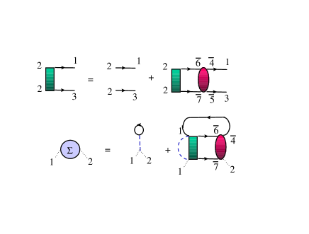
FIG. 1.: The first line is a skeleton diagram representation of the Bethe-Salpeter equation for the susceptibility in the particle-particle channel (Eq.(46) of accompanying paper[37]) and the second line is the corresponding equation for the self-energy (Eq.(58) of accompanying paper[37]). In the Hubbard model, the Fock contribution is absent, but in general it should be there. Solid lines are Green’s functions and dashed lines represent the contact interaction U. The box and attached lines are the particle-particle susceptibility while the ellipse is the irreducible particle-particle vertex. The particle-particle susceptibility is obtained by identifying points $1$ and $3$ in the Bethe-Salpeter equation.

With this approximation, the particle-particle susceptibility, which obeys the Bethe-Salpeter equation illustrated on the first line of Fig.1, can now be written as,

$$\chi_{p}^{\left(1\right)}(q)=\frac{\chi_{0}^{\left(1\right)}(q)}{1+U_{pp}\chi_{0}^{\left(1\right)}(q)}$$ (3)

where the irreducible particle-particle susceptibility is defined as

$$\chi_{0}^{\left(1\right)}(q)=\frac{T}{N}\sum_{k}G_{\sigma}^{\left(1\right)}(q-k)G_{-\sigma}^{\left(1\right)}(k)\;.$$ (4)

The vertices and the Green functions in $\chi_{p}^{\left(1\right)}(q)$ are at the same level of approximation in the sense that the irreducible vertex $U_{pp}$ is obtained from the functional derivative of the self-energy entering $G^{\left(1\right)}$. The vertex $U_{pp}=\left(\delta\Sigma/\delta G\right)$ is a constant and $\Sigma^{\left(1\right)}$ in zero external field is also a constant, leading to a Green function that has the same functional form as the non-interacting Green-function $G^{0}(k),$ where $k=\left(ik_{n},\vec{k}\right)$ stands for both the fermionic Matsubara frequency $ik_{n}$ and the wave vector $\vec{k}.$ The constant self-energy $\Sigma^{\left(1\right)}$ can be absorbed in the chemical potential by working at constant filling. If needed, we have argued in the accompanying paper[37] that the following should provide a useful approximation for $\Sigma^{\left(1\right)}$ since it allows the first-moment sum rule for the pair susceptibility to be satisfied [37],

$$\Sigma^{\left(1\right)}\simeq\frac{U}{2}-\frac{U_{pp}\left(1-n\right)}{2}$$ (5)

At this first level of approximation, only the double occupancy ($D\equiv\langle n_{\uparrow}n_{\downarrow}\rangle$) is needed to obtain the irreducible vertex $U_{pp}$ and hence the pairing fluctuations. The value of $\langle n_{\uparrow}n_{\downarrow}\rangle$ can be borrowed from some exact calculations or approximate estimates but, as in the repulsive case, we found that accurate results are obtained when $\langle n_{\uparrow}n_{\downarrow}\rangle$ is determined self-consistently from the following “local-pair sum rule”, a consequence of the fluctuation-dissipation theorem for the $s$-wave pairing susceptibility

$$\frac{T}{N}\sum_{q}\chi_{p}(q)\exp(-iq_{n}0^{-})=\langle\Delta^{\dagger}\Delta\rangle=\langle n_{\uparrow}n_{\downarrow}\rangle~{}.$$ (6)

Substituting $\chi_{p}^{\left(1\right)}$ Eq.(3) for the pair susceptibility and Eq.(2) for the irreducible vertex $U_{pp}$ leads to an equation that determines double-occupancy, and hence $U_{pp},$ self-consistently

$$\frac{T}{N}\sum_{q}\frac{\chi_{0}^{\left(1\right)}(q)}{1+U\frac{\langle(1-n_{\uparrow})n_{\downarrow}\rangle}{\langle 1-n_{\uparrow}\rangle\langle n_{\downarrow}\rangle}\chi_{0}^{\left(1\right)}(q)}\exp(-iq_{n}0^{-})=\langle n_{\uparrow}n_{\downarrow}\rangle~{}.$$ (7)

This first part of the calculation is referred to as the Two-Particle Self-Consistent (TPSC) approach.[44]

Once the pair susceptibility has been found, as above, the next step of the approach consists in improving the approximation for the single-particle self-energy by starting from an exact expression where the high-frequency Hartree-Fock behavior is singled out. This expression is represented by skeleton diagrams on the second line of Fig.(1). The piece of the exact self-energy that is added to the Hartree-Fock behavior represents low-frequency corrections. These involve Green functions, vertices and pair susceptibility for which we already have good approximations from the first step of the calculation. One thus substitutes in the exact expression the irreducible low frequency vertex $U_{pp}$ as well as all the other quantities at the same level of approximation, namely $G_{\sigma}^{\left(1\right)}(k+q)$ and $\chi_{p}^{\left(1\right)}(q)$ computed above, obtaining in Fourier space

$$\Sigma_{\sigma}^{\left(2\right)}(k)=Un_{-\sigma}-U\frac{T}{N}\sum_{q}U_{pp}\chi_{p}^{\left(1\right)}(q)G_{-\sigma}^{\left(1\right)}(q-k),$$ (8)

where $q=\left(iq_{n},\overrightarrow{q}\right)$ stands for both the bosonic Matsubara frequency and the wave vector. Here $T$ is the absolute temperature. The resulting self-energy $\Sigma_{\sigma}^{\left(2\right)}(k)$ on the left hand-side is at the next level of approximation so it differs from the self-energy entering the right-hand side. Physically, it is a self-energy coming from taking into account cooperons. As stressed previously[32, 33], it is important that the irreducible vertex $U_{pp},$ (or $\Gamma^{\left(1\right)}$) as well as $G_{\sigma}^{\left(1\right)}(k+q)$ and $\chi_{p}^{\left(1\right)}(q)$ all be at the same level of approximation otherwise some results, in particular with regards to the pseudogap, may come out qualitatively wrong.

The particle-particle irreducible vertex $U_{pp}$ may be regarded as the renormalized interaction strength containing vertex corrections. Note that in the expression for the self-energy $\Sigma^{\left(2\right)}$, Eq.(8), one of the vertices is bare while the other one is dressed with the same[45] particle-particle irreducible vertex function $U_{pp}$ that appears in the paring susceptibility. In other words, we do not assume that a Migdal theorem applies. If this had been the case, the self-energy would have, amongst other things, been proportional to $U^{2}$ instead of $UU_{pp}.$ In $T$-matrix theory the bare $U$ is used everywhere which, in particular, leads to a finite-temperature phase transition at the mean-field temperature. In our case, as described below, we proceed differently, avoiding altogether a finite-temperature phase transition in two-dimensions.

We briefly summarize some of the constraints satisfied by the above non-perturbative approach[37]. In Eq.(6), $\Delta$ is the local $s-$wave order parameter $c_{i\downarrow}c_{i\uparrow}$. Anti-commutation relations, or equivalently the Pauli principle, imply that $\langle\left[\Delta,\Delta^{\dagger}\right]\rangle=1-n.$ This in turn means that the convergence factor $\exp(-iq_{n}0^{-})$ in the local-pair sum rule is necessary because $\langle\left[\Delta,\Delta^{\dagger}\right]\rangle=1-n$ implies that, except at $n=1$, one needs to specify if $\tau=0^{+}$ or $\tau=0^{-}$ in the imaginary-time pair susceptibility. Either one of these limits however leads to the same value of $U_{pp}$ since our approach[37] satisfies exactly this consequence of the Pauli principle[46]: $\langle\left[\Delta,\Delta^{\dagger}\right]\rangle=1-n$. In complete analogy with the repulsive case discussed in Ref.[41], one can invoke the 2D phase space factor, $2\pi qdq$, and the Ornstein-Zernicke form of the pairing correlation function near a critical point to show the following. Deep in the renormalized classical regime, where the characteristic frequency $\nu_{c}$ of the retarded pairing susceptibility satisfies $\nu_{c}\lesssim T,$ the superconducting correlation length $\xi$ increases exponentially $\xi\sim exp(C/T)$ with decreasing temperature. In the latter expression, $C$ may be temperature dependent. This behavior is the one expected in the $O\left(n=\infty\right)$ universality class [47] and not in the $XY$, or $O\left(2\right),$ universality class, where $\xi_{BKT}\sim exp(C/\left(T-T_{BKT}\right)^{1/2}).$ The precise dependence on temperature of the correlation length in the temperature range between the beginning of the renormalized-classical regime and the actual critical regime is not known analytically. In the regime that we explore, the pseudogap begins to open at a temperature $T$ that is quite a bit larger than $T_{BKT}.$ The latter was estimated to be at most of order of $0.1t$ for $|U|=4$ by Moreo et al. [48]. As in the repulsive case, we will see below that the pseudogap appears in $A(\overrightarrow{k}_{F},\omega)$ if the pairing correlation length grows faster with decreasing temperature than the single-particle thermal de Broglie wavelength $\xi_{th}=v_{F}/T.$

B Comparisons with Monte Carlo calculations

In this section we show, by comparing with Monte Carlo calculations, that the present non-perturbative approach is an accurate approximation. The calculations are performed for the same lattice size as the corresponding Monte Carlo calculations. It is important to note that at half-filling the Lieb-Mattis canonical transformation $c_{i\downarrow}\rightarrow\exp\left(-i\overrightarrow{Q}{\bf\cdot}\overrightarrow{r}_{i}\right)c_{i\downarrow}^{\dagger}$, with $\overrightarrow{Q}=\left(\pi,\pi\right)$, maps the attractive model onto the repulsive one, pair fluctuations at wave vector $\overrightarrow{q}$ being mapped onto transverse spin fluctuations at wave vector $\overrightarrow{q}+\overrightarrow{Q}.$ With the proviso that in the attractive model at half-filling one would need, because of symmetry[33][51], to take into account the charge fluctuations, we can state that the comparisons done in the repulsive case[32][33] apply for the canonically equivalent attractive case. We note in particular that it was shown that the convergence to the infinite-size limit is similar in the Monte Carlo and in the non-perturbative approach[33]. We restrict our discussion to cases away from half-filling. The Quantum Monte Carlo simulations[52][53] that we performed were done using a Trotter decomposition with increment $\Delta\tau=1/10$ in imaginary time and the determinantal approach[54]. Typically, about $10^{5}$ or more Monte Carlo sweeps of the space-time lattice are performed.

We begin with double occupancy. Table I shows the value of double occupancy calculated from Monte Carlo simulations for various temperatures and fillings. The last column shows the value obtained from the self-consistent equation for double-occupancy Eq.(7).

FIG. 2.: (a) Double occupancy D calculated from the ansatz (solid curves), from the BCS ground state (dashed lines), and from the QMC simulations (circles) for $|U|=4$ at $n=0.5$ and 0.8. (b) Renormalized interaction strength $|U_{pp}|$ as a function of bare $|U|$ for $T=0.222$ at $n=0.5$. The dashed line is $U_{pp}=U$.

TABLE I.: Double occupancy for various fillings $n$ and temperature $\beta$ obtained from QMC calculations and from the TPSC approach. The systematic error in the QMC calculation is of order $1\%$, larger than the statistical uncertainty

$U$	$n$	$\beta$	QMC	TPSC
$-4$	$0.8$	$4$	$0.2671\pm 10^{-4}$	$0.273$
$-4$	$0.8$	$6$	$0.2703\pm 10^{-4}$	$0.288$
$-4$	$0.55$	$4$	$0.1561\pm 10^{-4}$	$0.157$
$-4$	$0.55$	$6$	$0.1590\pm 10^{-4}$	$0.169$

Clearly the accuracy of the approximation deteriorates at low temperature. This is illustrated by Fig.2(a) where, for both densities studied, the solid line starts to deviate from the Monte Carlo data around $\beta<5.$ As in the repulsive case, this occurs because the self-consistent expression for double-occupancy Eq.(7) fails once we enter the renormalized-classical regime where a pseudogap appears. Following Ref.[55], we expect that the pseudogap in $A(\overrightarrow{k}_{F},\omega)$ opens up as a precursor of Bogoliubov quasiparticles in the $BSC$ ground state. Since this ground state starts to control the Physics, it is natural to expect that a high-energy quantity such as $D$ should, in the pseudogap region, take the zero temperature $BCS$ value, namely

$$\langle n_{\uparrow}n_{\downarrow}\rangle=(\frac{1}{N}\sum_{\vec{k}}v_{\vec{k}}^{2})^{2}+(\frac{1}{N}\sum_{\vec{k}}u_{\vec{k}}v_{\vec{k}})^{2}\;,$$ (9)

where

$$u_{\vec{k}}^{2} = \frac{1}{2}(1+\frac{\varepsilon_{\vec{k}}-\mu}{E_{\vec{k}}})$$ (10)

$$v_{\vec{k}}^{2} = \frac{1}{2}(1-\frac{\varepsilon_{\vec{k}}-\mu}{E_{\vec{k}}})$$ (11)

$$E_{\vec{k}} = \sqrt{(\varepsilon_{\vec{k}}-\mu)^{2}+\Delta^{2}}\;.$$ (12)

with $\Delta$ the BCS mean-field gap. The chemical potential $\mu$ and gap $\Delta$ are determined self-consistently through the number and gap equations for given $U$, $T$ and $n$. The value of $D$ obtained with this approach is plotted as a dotted line in Fig.2(a), where it is apparent that the agreement with Monte Carlo calculations is excellent. In fact, for $\left|U\right|>3,$ the agreement is always at the few percent level. For smaller $\left|U\right|$, deviations occur, probably because at small coupling the order parameter at $\vec{q}{\bf=}0$ does not dominate anymore the sum over all wave vectors in $1/N\sum_{\vec{q}}\langle\Delta(\vec{q})^{\dagger}\Delta(-\vec{q})\rangle=\langle\Delta^{\dagger}\Delta\rangle=\langle n_{\uparrow}n_{\downarrow}\rangle$. In fact, as we shall see below, a good estimate of double-occupancy may also be obtained at small $U$ just from second-order perturbation theory. Now consider the temperature dependence of double-occupancy. The dependence predicted by the finite-temperature BCS result is on a scale $T=1$ at $|U|=4.$ That temperature dependence is clearly wrong for our problem since above $T_{MF}$ the BCS approach would give us back the non-interacting value. Hence the BCS result may be used only in the following way. For $\left|U\right|>3$ we can use the $T=0$ value of $\langle n_{\uparrow}n_{\downarrow}\rangle$ in the pseudogap region and the self-consistent value Eq.(2) above it. In the general case, $\langle n_{\uparrow}n_{\downarrow}\rangle$ does depend on temperature in the pseudogap regime, but that dependence should be relatively weak, as discussed in the repulsive case.[32]

We stress, however, that deep in the pseudogap regime our approach becomes eventually inaccurate when we obtain $\langle n_{\uparrow}n_{\downarrow}\rangle$ from the self-consistent equation (7). The reason for the loss of accuracy is analogous to that found at $n=1$ in the repulsive[32] case: In the present $U<0$ case, $\langle n_{\uparrow}n_{\downarrow}\rangle\rightarrow\langle n_{\downarrow}\rangle$ as $T\rightarrow 0$ to prevent a finite temperature phase transition. The approach also eventually becomes less accurate in the pseudogap regime when we take $\langle n_{\uparrow}n_{\downarrow}\rangle$ from BCS, but the fact that a more physically reasonable value of $\langle n_{\uparrow}n_{\downarrow}\rangle$ may be obtained in that case at $T=0$ helps extrapolate a little bit deeper in the pseudogap regime. The internal accuracy check discussed at the end of this section helps quantify the region of validity of the approach.

Before moving on with the comparisons, a few comments on the actual renormalized interaction strength $|U_{pp}|$ resulting from the Two-Particle Self-Consistent calculation. In Fig.2(b) $|U_{pp}|$ (denoted as stars) is plotted for $T=0.222$ as a function of bare $U$ by using the self-consistent expressions Eqs.(2) and (7). For this temperature, $U_{pp}$ approaches bare $U$ for $|U|\leq 1$ while in the intermediate coupling regime $1\leq|U|<\mbox{bandwidth}$ one notices a strong deviation from the bare $\left|U\right|.$ This deviation of $U_{pp}$ from $U$ makes a drastic difference, in particular in the two-particle function $\chi_{p}\left(\vec{q}\right)$ which ultimately governs the particle dynamics, including the pseudogap behavior. The saturation of $\left|U_{pp}\right|$ in Fig.2(b) signals the onset of the strong-coupling regime inaccessible in our approach that does not take into account the strong frequency dependence of vertices and self-energy present in this limit.

FIG. 3.: Calculated s-wave paring structure factor $S(\vec{q},\tau=0)$ (filled triangles) and QMC $S(\vec{q},\tau=0)$ (circles) for $|U|=4$ and various temperatures. (a) at $n=0.5$ and (b) at $n=0.8$ on a $8\times 8$ lattice. The dashed lines are to guide the eye..

Our approach gives a very accurate result for double-occupancy, but what about correlation functions? Another two-particle quantity related to the susceptibility is the pair structure factor. In Fig.3 the calculated s-wave pair structure factor (filled triangles) $S(\vec{q},\tau=0)\equiv$ $\langle\Delta(\vec{q})\Delta^{\dagger}(-\vec{q})+\Delta(\vec{q})^{\dagger}\Delta(-\vec{q})\rangle,$ where $\Delta(\vec{q})^{+}=\frac{1}{\sqrt{N}}\sum_{\vec{k}}c_{\vec{q}-\vec{k},\uparrow}^{+}c_{\vec{k},\downarrow}^{+},$ is compared with our QMC results (circles) for $|U|=4$ at $n=0.5$ (top panel) and $0.8$ (bottom panel) on a $8\times 8$ lattice. As the temperature decreases, the $\vec{q}=0$ mode becomes more singular in both results, a characteristic feature for growing s-wave pairing fluctuations. In most of the Brillouin zone, the agreement is excellent, in particular, for $n=0.5$ where the maximum difference is less than $10\%$ (Fig. 3(a)). For $n=0.8$ our calculated structure factor overestimates QMC results at most by $20\%$.

FIG. 4.: Comparison of the chemical potential shifts $\mu^{(1)}-\mu_{0}$ (open diamonds) and $\mu^{(2)}-\mu_{0}$ (open squares) with the results of QMC calculations (open circles), all done on a $8\times 8$ lattice. QMC error is a few percent, smaller than the open circles. Upper set of points are for $n=0.6$, and lower set of points are for $n=0.95$. For $n=0.6$, many-body calculations for a $64\times 64$ lattice are also illustrated by filled squares for $\mu^{(2)}-\mu_{0}$ , and by filled diamonds for $\mu^{(1)}-\mu_{0}$. In all cases, $\mu^{(2)}-\mu_{0}$ is closer to QMC data than $\mu^{(1)}-\mu_{0}$.

At the first level of approximation, we can also estimate the interaction-induced shift in chemical potential by starting from our approximate expression for the self-energy $\Sigma^{\left(1\right)}$, Eq.(5). Let us call the corresponding chemical potential $\mu^{\left(1\right)}=\mu_{0}+\Sigma^{\left(1\right)}.$ Our best estimate of single-particle quantities is obtained from the self-energy at the second level of approximation, Eq.(8). The corresponding chemical potential $\mu^{\left(2\right)}$ is calculated by requiring that the filling be the same as the one used at the first level of approximation. This procedure is identical to that for the repulsive model[56] and was suggested by Luttinger. It is discussed also in Sec.IV-C of the accompanying paper.[37] Figure 4 illustrates how the two estimates for the chemical potential on a $8\times 8$ lattice converge towards the value obtained from QMC calculations for the same size lattice. Consider the data for filling $n=0.6,$ in the upper part of the figure. The open squares, representing $\mu^{\left(2\right)}-\mu_{0},$ agree, within the error bars, with the QMC data represented by open circles. The first estimate for the chemical potential shift $\mu^{\left(1\right)}-\mu_{0}$ (open diamonds) starts to deviate from both the QMC data (open circles) and from $\mu^{\left(2\right)}-\mu_{0}$ (open squares) at the temperature where the pseudogap opens up (see Fig.12 below). Below this temperature, the self-energy becomes strongly frequency and momentum dependent, a feature captured by our improved estimate $\Sigma^{\left(2\right)}$ for the self-energy, but not by our first estimate, $\Sigma^{\left(1\right)}.$ The filled squares ($\mu^{\left(2\right)}-\mu_{0}$) and filled diamonds ($\mu^{\left(1\right)}-\mu_{0}$) were obtained for a $64\times 64$ lattice. They illustrate that one should compare finite-size QMC calculations to many-body calculations done on same size systems. They also illustrate that the second estimate for the chemical potential shift (squares) is more sensitive to system size. This is expected from the fact that it is only at the second level of approximation that the pseudogap appears for large correlation lengths. Let us now move to the lower part of Fig.4, where results closer to half-filling are plotted. The chemical potential there is very close to its exact temperature-independent half-filling value, $U/2,$ hence there is not much room to see the difference between the first and second estimate for the chemical potential. Nevertheless, even for $n=0.95$, the second estimate (open squares) is closer to the QMC data (open circles) than the first estimate (open diamonds).

We now compare the momentum distribution, a static quantity, obtained from QMC and from our analytical approach at the second level of approximation $\Sigma^{\left(2\right)}$.

FIG. 5.: The momentum dependent occupation number $n(\vec{k})$ for $|U|=4$ and $n=0.5$ at $T=0.25$. The circles denote $n(\vec{k})$ from QMC calculations by Trivedi et al. [57] on a $16\times 16$ lattice. The solid curve is calculated according to the equations given in this paper, while the dashed one is computed by replacing $U_{pp}$ by $U$ in the self-energy with all the rest unchanged. The long-dash line is the result of a self-consistent T-matrix calculation, and the dot-dash line the result of second-order perturbation theory.

The momentum dependent occupation number $n(\vec{k})$ (solid curve) is plotted in Fig. 5 along with the QMC calculations (circles) by Trivedi et al.[57] for a $16\times 16$ lattice, in a regime where the size dependence is negligible. The momentum distribution $n(\vec{k})$ drops rapidly near the Fermi surface, corroborating that for $|U|=4$ the electrons are in the degenerate state, instead of in the non-degenerate state of the strong coupling regime or of the preformed-pair scenario. The agreement between the non-perturbative method and QMC is clearly excellent. If we had assumed a Migdal theorem and taken $U^{2}$ instead of $UU_{pp}$ in Eq.(8) for the self-energy, then we would have obtained the dotted curve, which in absolute value differs as much from the QMC result as a non-interacting Fermi distribution would. Clearly Migdal’s theorem does not apply for this problem. In addition, Fig.5 also shows (long dashes) that a self-consistent $T-$matrix calculation does not compare to Monte Carlo data as well as our approach. Similarly, second-order perturbation theory (dot-dash) does not do well.

In Fig. 6 we present the total density of states $N^{-1}\sum_{\overrightarrow{k}}A(\overrightarrow{k},\omega)$ for $U=4$ and $n=0.87$ on an $8\times 8$ lattice and compare with existing QMC calculations by Moreo et al.[58]

FIG. 6.: The single-particle density of states for $|U|=4$ and $n=0.87$ at different temperatures on a $8\times 8$ lattice. (a) $T=1/2$, (b) $T=1/4$, (c) $T=1/6$, and (d) $T=1/8$. Both the solid line obtained from many-body calculations and the dashed line taken from the QMC calculations of Ref.[58] are obtained by analytic continuation of imaginary-time data using maximum entropy. The absolute error chosen for the Maximum Entropy continuation of the imaginary time many-body Green function for panels (a) to (d) is, respectively, $0.003,0.004,0.003,0.001$.

The many-body non-perturbative calculation is done in Matsubara frequency and analytically continued to real frequency using the same Maximum Entropy (ME) technique that is used for QMC calculations.[59] This allows us to smooth out the results in the same way as in the QMC calculation, namely by including statistical uncertainties in our imaginary-time data. This procedure was discussed in Ref.[33]. The uncertainties in the QMC data[58] that are presented in Fig.6 were not quoted. Hence, we chose the statistical uncertainties in the corresponding many-body calculations in such a way that the calculations presented in Fig.6(d) have the same degree of smoothness as the corresponding QMC data. More specifically, these uncertainties are of order $0.003$ on the absolute value of the imaginary time Green functions, which is typical of Monte Carlo calculations. At $T=1/2$ the density of states is similar to that for the non-interacting system. At $T\leq 1/4$, however, the spectral weight near the Fermi energy begins to be suppressed significantly with decreasing temperature, leading to a pseudogap. The small shoulders in the intermediate frequency regime for $T=1/6$ and $1/8$ come from finite size effect. When we use a $64\times 64$ lattice, these shoulders completely disappear.

In the case of the single-particle spectral weight, the latest QMC calculations at $n=1$[33] included studies of the finite-size effects, of the imaginary-time discretisation and of the uncertainties induced by the size of the Monte Carlo sample. They have shown that, at half-filling, there is indeed a pseudogap, in contrast to earlier findings [36]. Detailed comparisons with the many-body approach analog to the present one have been done. Although these studies were for the repulsive model, at half-filling the results apply for the attractive model since they are canonically equivalent at $n=1.$ One only needs to generalize the many-body approach to include the presence of the $SO\left(3\right)$ symmetry, as done in Ref.[33]. Slightly away from half-filling, namely for $n=0.95,$ QMC simulations[51][60] have found that a similar pseudogap opens up for $U=-4$ at a temperature large enough that the $SO\left(3\right)$ symmetry present at half-filling is barely broken $\left(T_{X}\gg\mu\right).$

Here we present results for $A(\overrightarrow{k},\omega)$ and for the total density of states $N\left(\omega\right)=N^{-1}\sum_{\overrightarrow{k}}A(\overrightarrow{k},\omega)$ at $n=0.8,$ $U=-4$ and two different temperatures, $T=0.25$ and $T=0.2,$ in the pseudogap regime. For that filling, finite-size studies are complicated by the fact that the available wave vectors do not necessarily coincide with the non-interacting Fermi surface. The closest such wave vector, $\overrightarrow{k}=\left(0,3\pi/4\right)$, is the one chosen for comparisons of $A(\overrightarrow{k},\omega)$. The results of QMC calculations are shown in Fig.(7) as dashed lines and those of the many-body approach as solid lines for the same $8\times 8$ system size.

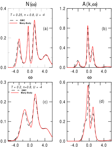
FIG. 7.: Total density of states (first column) and single-particle spectral weight at wave vector $(0,3\pi/4)$ (second column) are shown for $U=-4,n=0.8$ and two different temperatures. The lattice size is $8\times 8$. Dashed lines are the result of Maximum Entropy continuation of QMC data, and solid lines the result of Maximum Entropy continuation of many-body results with the same errors added in. Plots (a) and (b) on the first line are, respectively, $N(\omega)$ the total density of states, and $A(0,3\pi/4,\omega)$ the single-particle spectral weight at a point near the Fermi surface, for $T=0.25$. Panels (c) and (d) on the last line are the same plots but for $T=0.2$. The number of measurements done is $1.2\times 10^{5}$ for $T=0.25$ and $1.6\times 10^{5}$for $T=0.2$. In all cases, the absolute statistical error on the imaginary-time data is of order $2.0\times 10^{-3}$. Singular values less than $10^{-3}$ are dropped in the Maximum Entropy inversion.

The imaginary-time data corresponding to Fig.(7) appears in Fig.(8).

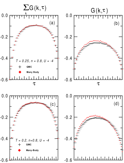
FIG. 8.: Imaginary-time data from which are extracted the density of states and spectral weights appearing in the respective panels of Fig.7. Error bars are shown only for the Monte Carlo data but the analytical data has been added the same errors as the Monte Carlo data.

  It is clear that all the main features of the Monte Carlo are seen by the many-body approach. The relative size of the split peaks at the Fermi surface is very sensitive to the actual location of the Fermi wave vector.

We conclude this section with the accuracy check described in the accompanying paper[37] and in previous work[32]. The question here is whether it is possible to find the domain of validity of the approach even in the absence of Monte Carlo data. The answer is given by Table II, where all results were computed for a $64\times 64$ lattice. One should focus on the three columns labeled Many-Body. In the first of these, one finds the value of $U\left\langle n_{\uparrow}n_{\downarrow}\right\rangle$ computed with TPSC, i.e. from Eq.(2) and the local-pair sum rule Eq.(7). That number is the same as that which would be obtained from Tr$\left[\Sigma^{\left(2\right)}G^{\left(1\right)}\right].$ However, finding by how much it differs from Tr$\left[\Sigma^{\left(2\right)}G^{\left(2\right)}\right]$, listed in the second column labeled Many-Body, gives an indication of how much the theory is internally consistent. The third column labeled Many-Body gives the absolute value of the relative difference between the first two Many-Body columns and it helps appreciate where the theory fails. Clearly, as temperature decreases and one enters the renormalized classical regime, the theory becomes invalid since the difference between $U\left\langle n_{\uparrow}n_{\downarrow}\right\rangle$ and Tr$\left[\Sigma^{\left(2\right)}G^{\left(2\right)}\right]$ starts to increase rapidly. As expected also, the theory is better at smaller coupling. Instead of computing $U\left\langle n_{\uparrow}n_{\downarrow}\right\rangle$ with the TPSC approach Eq.(7), one may also take it from the zero-temperature BCS value as described above. Comparing with the corresponding Many-Body columns, it is clear the BCS estimate of double occupancy does not compare as well with the TPSC result at small coupling, as explained above. In fact, in this region, second-order perturbation theory compares better. This is partly because the Hartree-Fock contribution to double-occupancy is dominant. The worse results for perturbation theory are for quarter filling at $U=-4$. Near half-filling it is known that second-order perturbation theory works well again. Note also that even if we start from the BCS result for $U\left\langle n_{\uparrow}n_{\downarrow}\right\rangle$, one can tell that the theory is becoming less accurate at too low temperature because, there again, $U\left\langle n_{\uparrow}n_{\downarrow}\right\rangle$ and Tr$\left[\Sigma^{\left(2\right)}G^{\left(2\right)}\right]$ begin to differ more and more from each other. This internal accuracy check, however, cannot tell us which approach is more accurate compared with QMC.

TABLE II.: Internal consistency check, for various $U$, $n$, and $T$ on a $64\times 64$ lattice. The three columns labeled Many-Body give, respectively, the value of $U<n_{\uparrow}n_{\downarrow}>$ obtained at the first level of approximation with the TPSC approach, that obtained at the second level of approximation from $Tr[\Sigma^{(2)}G^{(2)}]$ and the absolute value of the difference between the two results. The following column is Tr$\left[\Sigma G\right]$ obtained from second-order perturbation theory, and the last three columns are analogous to those where double-occupancy is obtained from the TPSC but they start from the $T=0$ BCS estimate of $U<n_{\uparrow}n_{\downarrow}>$.

			Many-Body	Many-Body	Many-Body	$2^{nd}order$	BCS	BCS	BCS
$U$	$n$	$T$	$U\left\langle n_{\uparrow}n_{\downarrow}\right\rangle$	Tr$\left[\Sigma^{\left(2\right)}G^{\left(2\right)}\right]$	$\left|diff\%\right|$	Tr$\left[\Sigma G\right]$	$U\left\langle n_{\uparrow}n_{\downarrow}\right\rangle$	Tr$\left[\Sigma^{\left(2\right)}G^{\left(2\right)}\right]$	$\left|diff\%\right|$
$-2$	$0.5$	$0.1$	$-0.1887$	$-0.1838$	$2.63$	$-0.1728$	$-0.1376$	$-0.1366$	$0.74$
$-2$	$0.5$	$0.2$	$-0.1892$	$-0.1861$	$1.61$	$-0.1743$	$-0.1376$	$-0.1371$	$0.39$
$-2$	$0.5$	$0.3$	$-0.1913$	$-0.1888$	$1.29$	$-0.1762$	$-0.1376$	$-0.1372$	$0.26$
$-2$	$0.5$	$0.4$	$-0.1939$	$-0.1917$	$1.15$	$-0.1787$	$-0.1376$	$-0.1373$	$0.19$
$-2$	$0.5$	$0.5$	$-0.1963$	$-0.1942$	$1.08$	$-0.1812$	$-0.1376$	$-0.1374$	$0.16$
$-2$	$0.5$	$1.0$	$-0.1988$	$-0.1970$	$0.88$	$-0.1875$	$-0.1376$	$-0.1375$	$0.10$
$-2$	$0.8$	$0.1$	$-0.4262$	$-0.4196$	$1.56$	$-0.4045$	$-0.3722$	$-0.3696$	$0.67$
$-2$	$0.8$	$0.2$	$-0.4274$	$-0.4226$	$1.11$	$-0.4090$	$-0.3722$	$-0.3706$	$0.41$
$-2$	$0.8$	$0.3$	$-0.4299$	$-0.4257$	$0.99$	$-0.4130$	$-0.3722$	$-0.3709$	$0.33$
$-2$	$0.8$	$0.4$	$-0.4320$	$-0.4280$	$0.93$	$-0.4166$	$-0.3722$	$-0.3711$	$0.28$
$-2$	$0.8$	$0.5$	$-0.4335$	$-0.4297$	$0.88$	$-0.4197$	$-0.3722$	$-0.3712$	$0.26$
$-2$	$0.8$	$1.0$	$-0.4313$	$-0.4284$	$0.66$	$-0.4248$	$-0.3722$	$-0.3714$	$0.20$
$-4$	$0.5$	$0.1$	$-0.6160$	$-0.5152$	$16.37$	$-0.4355$	$-0.5404$	$-0.4785$	$11.46$
$-4$	$0.5$	$0.2$	$-0.5427$	$-0.5067$	$6.64$	$-0.4412$	$-0.5404$	$-0.5050$	$6.55$
$-4$	$0.5$	$0.3$	$-0.5374$	$-0.5083$	$5.42$	$-0.4487$	$-0.5404$	$-0.5107$	$5.51$
$-4$	$0.5$	$0.4$	$-0.5406$	$-0.5131$	$5.08$	$-0.4578$	$-0.5404$	$-0.5129$	$5.08$
$-4$	$0.5$	$0.5$	$-0.5440$	$-0.5172$	$4.92$	$-0.4669$	$-0.5404$	$-0.5143$	$4.83$
$-4$	$0.5$	$1.0$	$-0.5385$	$-0.5168$	$4.03$	$-0.4897$	$-0.5404$	$-0.5184$	$4.07$
$-4$	$0.8$	$0.1$	$-1.2115$	$-1.0023$	$17.27$	$-0.9622$	$-1.0840$	$-0.9534$	$12.04$
$-4$	$0.8$	$0.2$	$-1.1042$	$-1.0179$	$7.82$	$-0.9786$	$-1.0840$	$-1.0070$	$7.10$
$-4$	$0.8$	$0.3$	$-1.0727$	$-1.0162$	$5.26$	$-0.9924$	$-1.0840$	$-1.0243$	$5.50$
$-4$	$0.8$	$0.4$	$-1.0685$	$-1.0185$	$4.68$	$-1.0048$	$-1.0840$	$-1.0302$	$4.96$
$-4$	$0.8$	$0.5$	$-1.0667$	$-1.0203$	$4.35$	$-1.0155$	$-1.0840$	$-1.0338$	$4.63$
$-4$	$0.8$	$1.0$	$-1.0462$	$-1.0126$	$3.21$	$-1.0349$	$-1.0840$	$-1.0441$	$3.68$

III Pseudogap formation in the density of states and in $A\left(k_{F},\omega\right)$

In the first subsection below, we summarize previous work on pseudogap in the attractive Hubbard model. In the second subsection, we use the approach of section II A to study the conditions under which a pseudogap appears in the density of states and in $A(\overrightarrow{k}_{F},\omega).$

A Overview of some recent work

The effect of superconducting fluctuations on the density of states was studied long ago.[61] To elucidate further the Physics of pseudogap formation, especially in the single particle spectral weight, many theoretical studies have focused on the attractive Hubbard model. An exhaustive review may be found in Ref.[38]. Although the attractive Hubbard model is clearly not a realistic model for cuprates since it predicts an $s-$wave instead of a $d-$wave superconducting ground state, it is an extremely useful paradigm. Indeed, except for the lack of cutoff in the interaction, it is analogous to the BCS model and is the simplest many-body Hamiltonian that leads to superconductivity with a possible crossover from the BCS limit at weak coupling to the Bose-Einstein limit at strong coupling.[62] A key point, as far as we are concerned, is that it also represents the only Hamiltonian for which QMC simulations are available now as a means of checking the accuracy of approximate many-body calculations.

The conventional picture[62], based on mean-field ideas, is that in the weak coupling regime ($\left|U/t\right|\ll 1$) pairing and phase coherence happen at the same temperature while in the strong coupling regime ($\left|U/t\right|\gg 1$) phase coherence may occur at $T_{c}$ much lower than $T^{\ast}$ where pair formation happens. In the latter case, the Fermi surface is destroyed well before the superconducting transition occurs. Since the ARPES experiments suggest a relatively well-defined Fermi surface, it has been suggested [63, 57, 64] that at intermediate coupling it is possible to retain aspects of both the Fermi surface of weak coupling and the preformed pair ideas of strong coupling. These possibilities have been extensively studied by several groups using a number of approaches that we will crudely divide in two types, numerical and many-body approaches.

Previous numerical QMC work charted the phase diagram of the attractive Hubbard model[65, 48, 49, 50]. They have also investigated the pseudogap phenomenon from intermediate to strong coupling[66, 67, 68]. We stress that the Physics in strong coupling is different from the weak to intermediate coupling limit we will study below. On the weak-coupling side of the BCS to Bose-Einstein crossover, there have been numerical studies of BKT superconductivity[58, 50] as well as several discussions of pseudogap phenomena in the spin properties (susceptibility and NMR relaxation rate) and in the total density of states at the Fermi level.[63, 57, 66] We have studied, through Quantum Monte Carlo (QMC) simulations, the formation of a pseudogap in $A\left(k_{F},\omega\right)$ in the weak to intermediate coupling regime of interest here[39, 51]. The present work is in agreement with our earlier results, as will be discussed in the next subsection.

The many-body techniques that have been applied to the attractive Hubbard model in the weak to intermediate coupling regime are mostly $T$-matrix and self-consistent (Fluctuation Exchange Approximation) $T$-matrix approaches [69, 70, 71, 72]. Let us consider the pseudogap problem in the non-superconducting state. At low density[73, 74], or with additional approximations[75, 76], a pseudogap may be found. By contrast, when the $\vec{q}=0$ superconducting mode is relaxational, self-consistent $T$-matrix calculations[77] have failed to show a pseudogap in the one-particle spectral function $A\left(k_{F},\omega\right)=-2\mathop{\rm Im}G^{R}\left(k_{F},\omega\right)$, a dimension-independent result. In two-dimensions, this absence of pseudogap is in sharp contrast with various QMC results[39, 51] and with general physical arguments inspired by studies of the repulsive case[55][78], which have already stressed that space dimension is crucial in the Physics of pseudogap formation.

In the non self-consistent version of the $T$-matrix approximation however, a pseudogap can be found[79]. Nevertheless, since the $T$-matrix approximation takes into account the Gaussian (first nontrivial) fluctuations with respect to the “mean field state”, one important pathology of the $T$-matrix approximation in two dimensions is that the Thouless criterion for the superconducting instability occurs at a finite mean-field temperature $T_{MF}.$ In the very weak coupling regime, this is considered inconsequential since the relative difference between $T_{MF}$ and the Berezinskii-Kosterlitz-Thouless[80] temperature (BKT) $T_{BKT}$ is of order[81] $T_{MF}/E_{F}$. In the intermediate-coupling regime however, this argument fails and one of the questions that should be answered is precisely the size of the fluctuating region where a pseudogap is likely to occur.

By contrast with non self-consistent $T-$matrix calculations, self-consistent $T$-matrix approaches do have a large fluctuation region, but they assume a Migdal theorem which means they do not take vertex corrections into account in the self-energy formula and use self-consistent Green functions. In the same way as in the case of repulsive interactions [82][33], the failure to treat vertex corrections and fluctuations at the same level of approximation may lead to incorrect conclusions concerning pseudogaps in $A(\overrightarrow{k}_{F},\omega)$. Self-consistent calculations have in fact lead to the claim [85] that only $d-$wave superconductivity may have precursor effects in $A\left(k_{F},\omega\right)$ above the transition temperature while Monte Carlo calculations[39][51] have exhibited this pseudogap even in the $s-$wave case. Recently, it has been pointed out using a different approach [86] that in the intermediate-coupling regime and when the filling is low, it becomes possible to have a bound $\vec{q}=0$ pair. This Physics leads to a pseudogap in $A(\vec{k},\omega)$ but it requires strong particle-hole symmetry breaking and is not specific to two dimensions. This result is discussed further in the following subsection.

Some authors[19, 20, 21, 24] have included phenomenologically a BKT fluctuation region either in $T-$matrix like calculations, through Hubbard-Stratonovich transformation or otherwise[22]. These calculations allow for phase fluctuations in the presence of a non-zero expectation value for the magnitude of the order parameter. In such a case, there is generally a real gap in $A(\overrightarrow{k}_{F},\omega),$ and additional effects must be included to fill-in the gap to transform it into a pseudogap[38]. In the approach that we take, any $SO\left(n\geq 2\right)$ theory would give qualitatively the same result above either $T_{BKT}$ for $n=2$ or above $T=0$ for $n>2$. In addition, in our approach the magnitude of the order parameter still fluctuates. It is when both amplitude and phase fluctuations enter the renormalized-classical regime, i.e. become quasistatic, that a pseudogap may open up.

B Pseudogap formation in weak to intermediate coupling

In this section, we focus on the Physics of fluctuation-induced pseudogap in the single-particle spectral weight of the two-dimensional attractive Hubbard model. This Physics has been discussed in previous QMC[39, 51, 60] and analytical work[55] but the present quantitative approach, based on the equations of Sec.II A, allows us to do calculations that are essentially in the thermodynamic limit and that can be done sufficiently rapidly to allow us to address other questions such as the crossover diagram in the temperature-filling plane.

Since the cuprates are strongly anisotropic and may be considered as a quasi 2D systems, it is important to understand in detail the limiting case of two-dimensions. Mean-field theory leads to finite-temperature phase transitions even in low dimensional systems where breaking of continuous symmetries is strictly forbidden at finite temperatures (Mermin-Wagner theorem[87]). Thus in low dimensions, mean-field theory, or fluctuation theory based on the mean-field state, lead to qualitatively wrong results at finite temperatures. One of the particular features of 2D that is captured by our approach, as we will see below, is that the mean-field transition temperature is replaced by a crossover temperature below which the characteristic energy of fluctuations is less than temperature, the so-called renormalized-classical regime. In this regime, the correlation length ($\xi$) increases exponentially until, in the superconducting case, one encounters the BKT[80] topological phase transition. As a result we find that when $\xi\gg v_{F}/T,$ the electronic system simulates the broken-symmetry ground state ($\xi=\infty$) at temperatures that are low but not necessarily very close to the transition temperature, leading to precursors of Bogoliubov quasiparticles[55] above $T_{c}$. Recent dimensional-crossover studies using an analogous approach[78] have suggested how the pseudogap will disappear when coupling to the third dimension is increased.

The results of this section for two-particle properties, such as the pairing susceptibility and the characteristic pairing fluctuation scale $\xi$, are all computed for an effective $2560\times 2560$ lattice. The one-particle properties are calculated instead for a $64\times 64$ lattice in momentum space. Fast Fourier transforms (FFT) were used in that case to speed up the calculations. The solid and long-dashed lines in Fig.9(b), obtained respectively for a $64\times 64$ and a $2560\times 2560$ lattice, illustrate that for single-particle properties a $64\times 64$ lattice suffices. This lattice size, for the temperatures we consider, is large enough[33] compared $\xi_{th}$ (panel in Fig.11(b)) that single-particle properties are essentially the same as they would be in the infinite-size limit. Refs.[31] and [33] discuss how single-particle properties become rather insensitive to system size even when $\xi>L$, as long as the condition $\xi_{th}<L<\xi$ is satisfied. This is discussed further in [89]. In the calculations, equation (7) is solved iteratively, then the self-energy Eq.(8) is obtained in Matsubara frequencies. The analytic continuation from Matsubara to real frequencies are performed via Padé approximants [90]. In order to detect any spurious features associated with this numerical analytical-continuation, we also performed real-frequency calculations. The results are identical, except for the fact that the Padé technique smooths out some of the spiky features of the real frequency formulation that are remnants of finite-size effects when the small imaginary part $\eta$ in retarded propagators is very small.

In Fig. 9 we show, for various temperatures, the total density of states (Fig. 9(a)) as well as the spectral function (Fig. 9(b)) $A(\overrightarrow{k}_{F},\omega)$ for the Fermi surface point crossing the $\left(0,0\right)-\left(\pi,0\right)$ line for $U=-4$ and quarter filling $n=0.5$

FIG. 9.: (a) The density of states and (b) the spectral function at the Fermi surface for $|U|=4$ and $n=0.5$ at different temperatures. The solid, dotted, dashed, long-dashed, and dot-dashed curves correspond to $T=0.143$, 0.182, 0.211, 0.308, and 0.364, respectively, except for panel (b) where the long-dashed line was calculated with a $2560\times 2560$ lattice to illustrate that size effects are small.

For $T=0.364$ (dot-dashed curve) the density of states, on the left panel, is similar to that for non-interacting electrons. With decreasing temperature below $T=0.32$, the low frequency spectral weight begins to be suppressed, leading to a pseudogap in the density of states. The condition for the appearance of a pseudogap in the spectral function $A(\overrightarrow{k}_{F},\omega)$, on the right panel, is more stringent than that in the total density of states. Although the pseudogap in the density of states is well developed for $T=0.211$ (dashed curve), it disappears in the spectral function for the same temperature. It is easier to form a pseudogap in the total density of states because of its cumulative nature: It suffices that scattering become stronger at the Fermi wave vector than at other wave vectors to push weight away from $\omega=0.$ Hence, a pseudogap may occur in the density of states even if $A(\overrightarrow{k}_{F},\omega)$ remains maximum at $\omega=0.$ This is what occurs in FLEX (Fluctuation Exchange) type calculations.[69, 72] It is more difficult to create a pseudogap in $A(\overrightarrow{k}_{F},\omega)$ itself since, at this wave vector, transforming a maximum at $\omega=0$ to a minimum requires the imaginary part of the self-energy to grow very rapidly as $T$ decreases.[32] The generality of these arguments suggests that $d-$wave pairing fluctuations, which were considered in Ref. [78, 88] for example, should also lead to a pseudogap in the density of states before a pseudogap in $A(\overrightarrow{k}_{F},\omega).$ This feature is consistent with the recent experimental observations[6] on high-temperature superconductors where pseudogap phenomena appear at higher temperatures in tunneling experiments than in ARPES experiments. Note also that with increasing temperature the pseudogap in both the density of states and the spectral function appears to fill instead of closing. This behavior is also in qualitative agreement with tunneling [6] and with ARPES experiments[3, 4]. All the above results are consistent with Monte Carlo simulations [60]. In addition to having found a pseudogap in the density of states [58], Fig.(6), the more recent Monte Carlo simulations done in the present and earlier papers [39][51] have also shown that a pseudogap may occur in $A(\overrightarrow{k}_{F},\omega)$ even in $s-$wave superconductors, contrary to the claims of Ref.[85].

Fig. 9(b) also shows one other qualitative result which is a clear signature of intermediate to strong-coupling systems, analogous to the signatures seen in optical spectra of high-temperature superconductors[83]. In changing $T$ by about $0.03$, from $0.21$ to $0.18,$ the spectral weight rearranges over a frequency scale of order one, i.e. over a frequency scale about $30$ times larger than the temperature change, and $5$ times larger than the absolute temperature $0.2$. In weak-coupling BCS theory, by contrast, spectral weight rearranges over a frequency scale of the order of the temperature change. The frequency range for spectral rearrangement observed in Fig. 9(b) would be even larger if the coupling was stronger.[84] This is a consequence of the fact that wave vector can be a very bad quantum number for correlated systems so that a momentum eigenstate can project on essentially all the true eigenstates of the system. The loss of meaning of momentum as a good quantum number and the corresponding spectral weight rearrangement over a large frequency scale happens suddenly in temperature in Fig. 9(b) because the correlation length becomes large at a rather sharp threshold temperature where the system becomes renormalized classical, as we now discuss.

Let us then demonstrate that the opening of the pseudogap in the single-particle density of states occurs when the pairing fluctuations enter the renormalized-classical regime.[39] In Fig. 10(a) the imaginary part of the paring susceptibility at $\vec{q}=0$ for $T=0.19$ and the characteristic frequency $\nu_{c}$ for pairing fluctuations are shown for $U=-4$ and $n=0.5$.

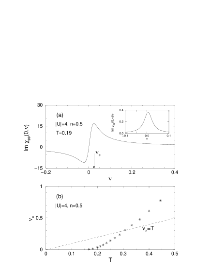
FIG. 10.: (a) The imaginary part of the pairing susceptibility at $\vec{q}=0$ for $T=0.19$ and (b) the characteristic low energy scale (stars) for pairing fluctuations at different temperatures for $|U|=4$ and $n=0.5$. The inset in (a) is the imaginary part of the pairing susceptibility divided by frequency at $\vec{q}=0$ for $T=0.19$.

Since for the parameters studied here the $\vec{q}=0$ mode is deep in the particle-particle scattering continuum, it has the characteristic frequency dependence of a relaxational mode, $1/(1-i\nu/\nu_{c}),$ that leads to a maximum in the imaginary part at some characteristic frequency $\nu_{c}$. Even though we do not have perfect particle-hole symmetry, the Fermi energy is still large enough compared with temperature that $\mathop{\rm Im}\chi_{pp}\left(0,\nu\right)/\nu$ is very nearly even (Inset in Fig. 10(a)). For other temperatures the behavior is similar. In Fig. 10(b) $\nu_{c}$ is plotted as a function of temperature. At high temperatures $\nu_{c}$ is larger than $T$ but below $T\simeq 0.31-0.32$ the characteristic frequency $\nu_{c}$ becomes smaller than $T$, signaling that we are entering the renormalized-classical regime. This phenomenon was also observed in QMC calculations.[39] In this regime, the thermal occupation number for pairing fluctuations is larger than unity. Clearly, the appearance of a pseudogap in the density of states in Fig. 9(a) follows very closely the entrance in the renormalized classical regime.

The present results should be contrasted with those of Levin’s group[86]. The pseudogap in their work comes from the presence of a $\vec{q}=0$ resonant pair state in the $T$-matrix. As the interaction strength decreases or the particle density increases, the $\vec{q}=0$ bound state enters into the particle-particle continuum, thereby acquiring a finite lifetime. As long as the $\vec{q}=0$ pair state is near the bottom of the scattering continuum it can remain a resonant state with a relatively long lifetime. Thus the origin of a pseudogap in their study is analogous to the preformed-pair scenario where the $\vec{q}=0$ pair is separated from the scattering continuum. Such a resonance corresponds to strong particle-hole asymmetry in the imaginary part of the pair susceptibility. In order to have such an asymmetry for moderate coupling strength, very small particle density is required in this approach. In our case, the pseudogap occurs even when the particle-hole symmetry is nearly perfect. Furthermore, in our case, other factors like density and interaction strength do not influence the results in any dramatic way. Low dimensionality is the key factor since phase space is behind the existence of both the renormalized classical regime and the very strong scattering of electrons on the corresponding fluctuations. The ratio $\xi/\xi_{th}$ controls the importance of this scattering[31] as we discuss in the following paragraph.

In Fig. 11 we contrast the onset of the pseudogap in the spectral function on the Fermi surface along different directions, namely the $(0,0)-(0,\pi)$ and $(0,0)-(\pi,\pi)$ directions, for $|U|=4$ and $n=0.5$.

FIG. 11.: Spectral function for $|U|=4$ and $n=0.5$ (a) along $(0,0)-(0,\pi)$ direction and (b) along $(0,0)-(\pi,\pi)$ direction. The inset in (b) shows the pairing correlation length (solid curve), and $\xi_{th}=v_{F}/T$ along $(0,0)-(\pi,\pi)$ direction (dotted curve) and $(0,0)-(0,\pi)$ direction (dashed curve) for the same parameters.

At this density, where the Fermi surface is nearly circular, the anisotropy happens in a very small temperature range around $T=0.19$. For $T=0.19$ (dotted curves), the figure shows that the pseudogap occurs only along the $(0,0)-(0,\pi)$ direction. This anisotropy of the pseudogap in the spectral function should be contrasted with the fact that in the superconducting state, the gap is isotropic. The anisotropy at the temperature where the pseudogap opens up can be understood following the arguments of Vilk et al.[32]. Using the dominant renormalized-classical fluctuations ($iq_{n}=0$), these authors showed that for $\xi\gg v_{F}/T$ the scattering rate (imaginary part of the self-energy) on the Fermi surface becomes large, leading to a minimum in the spectral function at $\omega=0$ instead of the maximum that exists in the absence of a pseudogap. In the inset of Fig.11(b) the pairing correlation length $\xi$, as well as $\xi_{th}=v_{F}/T$ along the $(0,0)-(\pi,\pi)$ and $(0,0)-(0,\pi)$ directions are plotted as a function of temperature. Clearly $\xi$ grows exponentially with decreasing temperature. Furthermore, according to the above criterion, a pseudogap in the spectral function exists along one direction and not along the other when $\xi$ (solid curve) is larger than $\xi_{th}$ along $(0,0)-(0,\pi)$ (dashed curve) but smaller than $\xi_{th}$ along the $(0,0)-(\pi,\pi)$ (dotted curve), namely, in the temperature range $0.175<T<0.185$. We obtain quantitative agreement with Fig. 11(b) if we use $\xi=1.3\xi_{th}$ as the criterion for the appearance of a pseudogap. While the pseudogap anisotropy happens in a narrow temperature range at this density due to the small Fermi velocity anisotropy (about $1.35$), closer to half-filling it occurs in a large temperature interval since the Fermi velocity is nearly vanishing close to the $(0,\pi)$ point.[51]

Finally in Fig. 12 we present the crossover diagram for the pseudogap in the 2D attractive Hubbard model for $|U|=4$.

FIG. 12.: The crossover diagram of the 2D attractive Hubbard model for $|U|=4$. The filled triangles and stars denote the temperatures where a pseudogap appears in the density of states and the spectral function, respectively. The solid lines are a guide to the eye. The dashed curve is the BCS mean field temperature $T_{MF}$ and the dotted curve is an estimate of the Kosterlitz-Thouless temperature $T_{KT}$ extracted from QMC results by Moreo et al. [48].

The dotted curve is a rough QMC[48] estimate (probably an upper bound) for the BKT transition temperature $T_{BKT}$. For all densities a pseudogap in the one-particle functions appears in a wide temperature range $T_{BKT}<T<T^{\ast}$ where $T^{\ast}$ is typically several times of $T_{BKT}=T_{c}$. The pseudogap occurs earlier in the density of states than in the spectral functions for most of densities. Near half-filling, however, the pseudogap appears more or less at the same temperature in the density of states and the spectral functions. In QMC for small systems, there seems to be a difference in the temperatures at which the two pseudogaps open up.[60] Performing a calculation with finite second neighbor hopping $t^{\prime},$ we have confirmed that this almost simultaneous opening of the pseudogaps happens because of the strong influence of the Van Hove singularity, which leads to $v_{F}=0,$ and not because of nesting.[91] Finally, note that at half-filling one has perfect $O\left(3\right)$ symmetry in this model so that the transition temperature vanishes, as dictated by the Mermin-Wagner theorem, while the pseudogap temperature continues to be large, following the trend of the mean-field transition temperature instead of that of the $T_{BKT}$ curve. This shows that symmetry of the order-parameter space contributes to enlarge the temperature range where the pseudogap occurs, as expected from the corresponding enlargement of the renormalized-classical regime.[51]

IV Conclusion

In weak to intermediate coupling, the attractive Hubbard model can be studied quantitatively with a non-perturbative approach[37] that directly extends the corresponding method for the repulsive model[41, 31, 32]. The simple equations of section II A are all that needs to be solved. This many-body approach has an internal accuracy check, no adjustable parameter and it satisfies several exact sum rules[37]. We have demonstrated the accuracy of this method through detailed comparisons of its predictions with Quantum Monte Carlo simulations of both single-particle and two-particle correlation functions.

On the Physical side, we studied the fluctuation-induced pseudogap that appears in the single-particle spectral weight, in agreement with Monte Carlo simulations and in close analogy with the results found before in the repulsive case[32][33]. A key ingredient for this pseudogap is the low dimensionality. Indeed, in two-dimensions the finite-temperature mean-field transition temperature is replaced by a crossover to a renormalized-classical regime where the characteristic pairing frequency is smaller than temperature and the pairing correlation length $\xi$ grows faster than the single-particle thermal de Broglie wavelength $\xi_{th}$. In this approach, where vertex corrections and Green functions are taken at the same level of approximation in the self-energy expression[32][33], the renormalized-classical fluctuations and the relatively large phase space available for them in two-dimensions lead to precursors of the superconducting gap (or Bogoliubov quasiparticles) in the normal state. This pseudogap can occur without resonance in the pair susceptibility[86], and it appears not only in the total density of states but also in the single-particle spectral weight, in sharp contrast with what was found with self-consistent $T-$matrix approaches[77]. Our approach fails at strong coupling or at low temperature very close to the Berezinskii-Kosterlitz-Thouless (BKT) transition.

For $\left|U\right|=4,$ the pseudogap regime occurs over a temperature scale that is several times the BKT transition temperature. The crossover to the renormalized-classical regime is about a factor of two lower than the mean-field transition temperature but it has the same filling dependence, which can be quite different from that of the real transition temperature, which is strongly dependent on the symmetry of the order-parameter space[51]. It is clear also that $SO\left(2\right)$ (or $U\left(1\right)$) symmetry is not essential to the appearance of a pseudogap. It would also appear if there happens to be a hidden continuous symmetry group [92][51] $SO\left(n\right)$ with $n\geq 2$ describing the high-temperature superconductors.

As stressed earlier in this paper, the attractive Hubbard model is not directly applicable to the cuprates. Nevertheless, it helps understand the nature of superconducting-fluctuation induced pseudogaps, if they happen to be present. The pseudogap appearing for the underdoped compounds at high temperature in thermodynamic and transport measurements, or at high energy in tunnelling[6] and ARPES experiments, is most probably not of pure superconducting origin[93][94]. Nevertheless, close enough to the superconducting transition, in both the underdoped and overdoped regions, there should be an effective model with attraction describing the low energy Physics. Since even the high-temperature superconductors have a gap to Fermi energy ratio that is small, this effective model could be a weak-coupling one (but not necessarily[95]). Time-domain transmission spectroscopy experiments[96] in the $100GHz$ range suggest that the renormalized classical regime for the BKT transition has been observed in underdoped compounds, $10K$ to $15K$ above $T_{c}$. Also, in the overdoped regime, recent experiments on the magnetic field dependence of NMR $T_{1}^{-1}$ and Knight shift[97] suggest that the pseudogap appearing a few tens of degrees above $T_{c}$ is indeed a superconducting-fluctuation induced pseudogap. The pseudogap that we have described should appear in these regimes if an effective weak to intermediate-coupling attractive-interaction model is valid near $T_{c}$. In this context, some of the important results that we found and explained are as follows. In the attractive Hubbard model the pseudogap appears earlier in the density of states than in the spectral function that would be measured by ARPES, as summarized in Fig.(12). We also found, Fig.(9), that with increasing temperature, spectral weight appears to fill in the pseudogap instead of closing it. Finally, we also showed that as the system enters the renormalized-classical regime, spectral weight can rearrange over a frequency range much larger than the temperature scale. This is generally a signature that momentum is becoming a very bad quantum number. Hence, for a given temperature scale, the frequency range over which the spectral weight can rearrange becomes larger with increasing coupling[84]. All these features carry over the $d-$wave case[78, 88]. Qualitative differences between weak- and strong-coupling pseudogaps have been discussed in Ref.[33].

- [1] T. Timusk, and B.W. Statt, Rep. Prog. Phys. 62, 61 (1999).
- [2] H. Mayaffre, P. Wzietek, C. Lenoir, D. Jérome, and P. Batail, Europhys. Lett. 28, 205 (1994); P. Wzietek, H. Mayaffre, D. Jérome, and S. Brazovskii, J. Phys. I France 6, 2011 (1996); K. Frikach, M. Poirier, M. Castonguay, and K. D. Truong , Phys. Rev. B 61, R6491 (2000).
- [3] A. G. Loeser, Z.-X. Shen, D.S. Dessau, D.S. Marshall, C.H. Park, P. Fournier, A. Kapitulnik, Science, 273, 325 (1996).
- [4] H. Ding, T. Yokoya, J.C. Campuzano, T. Takahashi, M. Randeria, M.R. Norman, T. Mochiku, K. Kadowaki, and J. Giapintzakis, Nature 382, 51 (1996).
- [5] J. W. Loram, K. A. Mirza, J. R. Cooper, and W. Y. Liang , Phys. Rev. Lett. 71, 1740 (1993); Physica (Amsterdam) 235C-240C, 134 (1994).
- [6] Ch. Renner, B. Revaz, J.-Y. Genoud, K. Kadowaki, and Ø. Fischer, Phys. Rev. Lett. 80, 149 (1998); N. Miyakawa, J. F. Zasadzinski,1, L. Ozyuzer, P. Guptasarma, D. G. Hinks, C. Kendziora, and K. E. Gray, Phys. Rev. Lett.83, 1018 (1999).
- [7] M. Takigawa, A. P. Reyes, P. C. Hammel, J. D. Thompson, R. H. Heffner, Z. Fisk, and K. C. Ott, Phys. Rev. B 43, 247 (1991); H. Alloul, A. Mahajan, H. Casalta, and O. Klein, Phys. Rev. Lett. 70, 1171 (1993).
- [8] Joseph Orenstein, G. A. Thomas, A. J. Millis, S. L. Cooper, D. H. Rapkine, T. Timusk, L. F. Schneemeyer, and J. V. Waszczak , Phys. Rev. B 42, 6342 (1990); L. D. Rotter, Z. Schlesinger, R. T. Collins, F. Holtzberg, C. Field, U. W. Welp, G. W. Crabtree, J. Z. Liu, Y. Fang, K. G. Vandervoort, and S. Fleshler , Phys. Rev. Lett. 67, 2741 (1991); C. C. Homes and T. Timusk, R. Liang, D. A. Bonn, and W. N. Hardy , Phys. Rev. Lett. 71, 1645 (1993).
- [9] P. W. Anderson, Science 235, 1196 (1987).
- [10] T. Tanamoto, K. Kohno, and H. Fukuyama, J. Phys. Soc. Jpn. 61, 1886 (1992).
- [11] P. A. Lee and X. G. Wen, Phys. Rev. Lett. 78, 4111 (1997).
- [12] J. Zaanen and O. Gunnarsson, Phys. Rev. B 40, 7391 (1989); D. Poilblanc and T.M. Rice, Phys. Rev. B 39, 9749 (1989); H.J. Schulz, J. Physique, 50, 2833 (1989); K. Machida, Physica C 158, 192 (1989); K. Kato et. al., J. Phys. Soc. Jpn. 59, 1047 (1990); J.A. Verges et. al., Phys. Rev. B 43, 6099 (1991); M. Inui and P.B. Littlewood, Phys. Rev. B 44, 4415 (1991); J. Zaanen and A.M. Oles, Ann. Physik 5, 224, (1996).
- [13] S.A. Kivelson and V.J. Emery, p. 619 in ”Proc. Strongly Correlated Electronic Materials: The Los Alamos Symposium 1993,” K.S. Bedell et. al., eds. (Addison Wesley, Redwood City, Ca., 1994).
- [14] C. Castellani, C. Di Castro, and M. Grilli, Phys. Rev. Lett. 75, 4 650 (1995).
- [15] Steven R. White, and D. J. Scalapino, cond-mat/0006071
- [16] S. Chakravarty, R. B. Laughlin, D. K. Morr, C. Nayak, cond-mat/0005443
- [17] S. Doniach and M. Inui, Phys. Rev. B 41, 6668 (1990).
- [18] V. J. Emery and S. A. Kivelson, Nature 374, 434 (1995).
- [19] V. M. Loktev, Rachel M. Quick, and S. G. Sharapov, Low Temp. Phys. 26 (in press), cond-mat/9904126; V.P. Gusynin, V. M. Loktev, and S. G. Sharapov, JETP Lett. 65, 182 (1997); Fiz. Nizk. Temp. 23, 816 (1997) (Engl. trans.: Low Temp. Phys. 23, 612 (1997)); JETP 88, 685 (1999); JETP Lett. 69, 141 (1999); JETP (2000) (in press) cond-mat/9811207.
- [20] J.O. Sofo, and C.A. Balseiro, Phys. Rev. B 45, 8197 (1992); J.J. Vincente Alvarez, and C.A. Balseiro, Solid State Comm. 98, 313 (1996).
- [21] D. Ariosa, and H. Beck, Phys. Rev. B 43, 344 (1991); Phys. Rev. B 45, 819 (1992); M. Capezzali, D. Ariosa, and H. Beck, Physica B 230-232, 962 (1997); D. Ariosa, H. Beck, and M. Capezzali, J. Phys. Chem. Solids 59, 1783 (1998); M. Capezzali, and H. Beck, Physica B 259-261, 501 (1999).
- [22] M. Franz and A. J. Millis, Phys. Rev. B 58, 14572 (1998).
- [23] Qijin Chen, Ioan Kosztin, Boldizsár Jankó, and K. Levin, Phys. Rev. Lett. 81, 4 708 (1998).
- [24] H. J. Kwon, and A. T.Dorsey, Phys. Rev. B 59, 6438 (1999).
- [25] A. M. Cucolo, M. Cuoco, and A. A. Varlamov, Phys. Rev. B 59, R11675 (1999).
- [26] P. Devillard, J. Ranninger, Phys. Rev. Lett. 84, 5200 (2000).
- [27] Z. X. Shen and J. R. Schrieffer, Phys. Rev. Lett. 78, 1771 (1997).
- [28] J. Schmalian, D. Pines, and B. Stojkovic, Phys. Rev. Lett. 80, 3839 (1998); A. V. Chubukov, cond-mat/9709221 (unpublished).
- [29] H. Ding, J.R. Engelbrecht, Z. Wang, J. C. Campuzano, S.-C. Wang, H.-B. Yang, R. Rogan, T. Takahashi, K. Kadowaki, D. G. Hinks, cond-mat/0006143
- [30] D.L. Feng, D.H. Lu, K.M. Shen, C. Kim, H. Eisaki, A. Damascelli, R. Yoshizaki, J.-I. Shimoyama, K. Kishio, G. Gu, S. Oh, A. Andrus, J. O’Donnell, J.N. Eckstein, and Z.X. Shen (Science, in press)
- [31] Y.M. Vilk and A.-M.S. Tremblay, Europhys. Lett. 33, 159 (1996): Y.M. Vilk et A.-M.S. Tremblay, J. Phys. Chem. Solids 56, 1769 (1995).
- [32] Y.M. Vilk and A.-M.S. Tremblay, J. Phys. I (France) 7, 1309 (1997).
- [33] S. Moukouri, S. Allen, F. Lemay, B. Kyung, D. Poulin, Y.M. Vilk and A.-M.S. Tremblay, Phys. Rev. B 61, 7887 (2000).
- [34] C. Huscroft, M. Jarrell, Th. Maier, S. Moukouri, A.N. Tahvildarzadeh, cond-mat/9910226. This work confirms our contention since by adding the effect of finite dimension through a cluster approach to dynamical mean-field theory, a pseudogap appears.
- [35] J. J. Deisz, D. W. Hess and J. W. Serene, Phys. Rev. Lett. 76, 1312 (1996).
- [36] M. Vekic and S. R. White, Phys. Rev. B 47, 1160 (1993).
- [37] S. Allen and A.-M.S. Tremblay, preceeding paper.
- [38] Vadim M. Loktev, Rachel M. Quick, and Sergei G. Sharapov (Physics Reports, in press)
- [39] Y.M. Vilk, S. Allen, H. Touchette, S. Moukouri, L. Chen and A.-M.S. Tremblay, J. Phys. Chem. Solids 59, 1873 (1998).
- [40] K.S. Singwi, M.P. Tosi, R.H. Land, and A. Sjölander, Phys. Rev. 176, 589 (1968). For a review, see K.S. Singwi and M.P. Tosi, Solid State Phys. 36, 177 (1981).
- [41] Y. M. Vilk, Liang Chen, and A.-M.S. Tremblay, Phys. Rev. B 49, 13 267 (1994).
- [42] Gordon Baym, Phys. Rev. 127, 1391 (1962).
- [43] This expression for Eq.(2) may also be obtained by canonical transformation to the attractive Hubbard model of the corresponding result obtained in the transverse spin channel for the repulsive model.
- [44] The name Two-Particle Self-Consistent (TPSC) is because the self-consistency in Eq.(7) involves the particle-particle irreducible vertex and a special case of the pair susceptibility. Consistency with for this Hamiltonian is trivial but it would also need to be taken into account for models more general than Hubbard’s.
- [45] If we take the point of view that is an average of the particle-particle irreducible vertex in the sense of the mean-value theorem for integrals, then the integrals in the Bethe-Salpeter equation and in the self-energy are over different variables so the in the numerator of the self-energy equation may be slightly different from the one entering the susceptibility, as discussed in Refs.[31] and [32]
- [46] More generally, the sum-rule is satisfied for all wave vectors .
- [47] Anne-Marie Daré, Y.M. Vilk and A.-M.S. Tremblay, Phys. Rev. B 53, 14 236 (1996).
- [48] A. Moreo and D. J. Scalapino, Phys. Rev. Lett. 66, 946 (1991).
- [49] D.J. Scalapino, S.R. White, S. Zhang, Phys. Rev. B 47, 7995 (1993).
- [50] F.F. Assaad, W. Hanke, and D.J. Scalapino, Phys. Rev. Lett. 71, 1915 (1993); Phys. Rev. B 49, 4 327 (1994).
- [51] S. Allen, H. Touchette, S. Moukouri, Y.M. Vilk, A.-M. S. Tremblay, Phys. Rev. Lett., 83, 4128 (1999).
- [52] J. E. Hirsh, Phys. Rev. B 31, 4403 (1985).
- [53] S. R. White, D.J. Scalapino, and R. L. Sugar, E. Y. Loh, Jr., J. E. Gubernatis, and R. T. Scalettar, Phys. Rev. B 40, 506 (1989).
- [54] R. Blankenbecler, D.J. Scalapino, et R.L. Sugar, Phys. Rev. D 24, 2278 (1981).
- [55] Section 5.6 of Y.M. Vilk and A.-M.S. Tremblay, J. Phys. I (France) 7, 1309 (1997).
- [56] Discussion below Eq.(47) in Ref.[31]
- [57] N. Trivedi and M. Randeria, Phys. Rev. Lett. 75, 312 (1995).
- [58] A. Moreo, D. J. Scalapino, and S. R. White, Phys. Rev. B 45, 7544 (1992).
- [59] R. K. Bryan, Eur. Biophys. J. 18, 165 (1990); M. Jarrell and J. E. Gubernatis, Phys. Rep. 269, 133 (1996).
- [60] S. Allen, PhD thesis, Université de Sherbrooke (unpublished).
- [61] Elihu Abrahams, Martha Redi, and James W.F. Woo, Phys. Rev. B 1, 208 (1970); B.R. Patton, Phys. Rev. Lett. 27, 1273 (1971). For a review, M. Ausloos, and A.A. Varlamov, in Fluctuation phenomena in high temperature superconductors (Kluwer Academic Publishers, Dordrecht, 1997).
- [62] P.Nozières and S.Schmitt-Rink, J. Low Temp. Phys. 59, 195 (19985).
- [63] Mohit Randeria, Nandini Trivedi, Adriana Moreo, and Richard T. Scalettar, Phys. Rev. Lett. 69, 2001 (1992).
- [64] M. Randeria, cond-mat/9710223 (Varenna Lectures, 1997).
- [65] R. T. Scalettar, E. Y. Loh and J. E. Gubernatis, A. Moreo, S. R. White, D. J. Scalapino, and R. L. Sugar, E. Dagotto, Phys. Rev. Lett. 62, 1407 (1989). A. Moreo, and D. J. Scalapino, Phys. Rev. Lett. 66, 946 (1991); M. Guerrero, G. Ortiz, and J. E. Gubernatis, Phys. Rev. B 62, 600 (2000).
- [66] J. M. Singer, M.H. Pedersen, T. Schneider, H. Beck, and H.G. Matuttis, Phys. Rev. B 54, 1286 (1996).
- [67] J.M. Singer, T. Schneider, and M.H. Pedersen, Eur. Phys. J. B 1, 1 (1998) and references therein.
- [68] J.M. Singer, T. Schneider, P.F. Meier, Eur. Phys. J. B 7, 37 (1999).
- [69] J. W. Serene, Phys. Rev. B 40, 10 873 (1989).
- [70] M.H. Pedersen, J.J.Rodríguez-Núñez, H. Beck, et al. Z. Phys. B 103, 21 (1997).
- [71] S. Shafroth, J.J.Rodríguez-Núñez, and H. Beck, J. Phys. (Cond. Mat.) 9, L111 (1997).
- [72] J. J. Deisz, D. W. Hess, and J. W. Serene, Phys. Rev. Lett. 80, 373 (1998).
- [73] M. Yu. Kagan, R. Frésard, M. Capezzali, H. Beck, Phys. Rev. B 57, 5995 (1998); R. Frésard, B. Glasser, and P. Wölfle, J. Phys. Cond. Matt. 4, 8565 (1992).
- [74] Bumsoo Kyung, E. G. Klepfish, and P. E. Kornilovitch, Phys. Rev. Lett. 80, 3109 (1998).
- [75] R. Micnas, M. H. Pedersen, S. Schafroth, T. Schneider, J. J. Rodríguez-Núñez and H. Beck , Phys. Rev. B 52, 16 223 (1995).
- [76] O. Tchernyshyov, Phys. Rev. B 56, 3372 (1997).
- [77] M. Letz, and R.J. Gooding, J. of Phys. Chem. Sol. 59, 1838 (1998); M. Letz, and R.J. Gooding, J. Phys. (Cond. Mat.) 10, 6 931 (1998); M. Letz, Proceedings of the ”XXII School of Theoretical Physics”, Ustron 98, cond-mat/9905018.
- [78] G. Preosti, Y. M. Vilk, and M. R. Norman, Phys. Rev. B 59, 1474 (1999).
- [79] K.S.D. Beach, R.J. Gooding, F. Marsiglio, cond-mat/9912177.
- [80] V.L. Berezinskii, Zh. Eksp. Teor. Fiz. 59, 907 (1970); J. M. Kosterlitz and D. J. Thouless, J. Phys. C 6, 1181 (1973).
- [81] B.I. Halperin and D.R. Nelson, J. Low Temp. Phys. 36, 599 (1979). We thank M. Randeria for pointing out this reference.
- [82] Section 6.2 of Y.M. Vilk and A.-M.S. Tremblay, J. Phys. I (France) 7, 1309 (1997).
- [83] A.S. Katz, S.I. Woods, E.J. Singley, T.W. Li, M. Xu, D.G. Hinks, R.C. Dynes, D.N. Basov, Phys. Rev. B 61, 5930 (2000); D.N. Basov, S.I. Woods, A.S. Katz, E.J. Singley, R.C. Dynes, M. Xu, D.G. Hinks, C.C. Homes, M. Strongin, Science, 283, 49 (1999).
- [84] Stéphane Pairault, David Senechal, A.-M. S. Tremblay, Euro. Phys. J. B 16, 85 (2000).
- [85] Jan R. Engelbrecht, Alexander Nazarenko, Mohit Randeria, Elbio Dagotto, Phys. Rev. B 57, 13 406 (1998)
- [86] Ioan Kosztin, Qijin Chen, Boldizsár Jankó, and K. Levin, Phys. Rev. B 58, R5936 (1998); B. Janko, J. Maly, and K. Levin, Phys. Rev. B 56, R 11407 (1997).
- [87] N. D. Mermin and H. Wagner, Phys. Rev. Lett. 17, 1133 (1966).
- [88] B. Kyung, cond-mat/0003492
- [89] The renormalized-classical contribution to the self-energy Eq.(8) is the one that is most sensitive to the large correlation length . In two dimensions, we know that on an infinite-size lattice one can approximate this contribution to by because is constrained by to be of order and (i.e. ). On a finite lattice, the same dependence for all will also follow when , i.e. when While the prefactor, could in principle be different on infinite and finite lattices, the fact that depends little on system size ensures that is basically system size independent since finite contributions to the sum rule Eq.(7) also are size independent.
- [90] H. J. Vidberg and J. W. Serene, J. Low Temp. Phys. 29, 179 (1977).
- [91] B. Kyung, unpublished
- [92] S.C. Zhang, Science, 275, 1089 (1997).
- [93] J.L. Tallon, and J.W. Loram, Submitted to Physica C, 2 May 2000, cond-mat/0005063
- [94] V.M.Krasnov, A.E.Kovalev, A.Yurgens, and D.Winkler, Phys. Rev. Lett. 84, 5860 (2000); J. L. Tallon and G. V. M. Williams Phys. Rev. Lett. 82, 3725 (1999).
- [95] Even though the attractive part of the Hamiltonian could be in the weak coupling regime, if there is a strongly repulsive term also in the Hamiltonian the details of the Physics near the superconducting transition could be quite different from what is found in the attractive Hubbard model. Nevertheless, the fact that we were able to treat the model up to intermediate coupling suggests that many of our qualitative results should hold in the more general case.
- [96] J. Corson, R. Mallozzi, J. Orenstein, J.N. Eckstein, and I. Bozovic, Nature, 398, 221 (1999).
- [97] Guo-qing Zheng, H. Ozaki, W. G. Clark, Y. Kitaoka, P. Kuhns, A. P. Reyes, W. G. Moulton, T. Kondo, Y. Shimakawa, and Y. Kubo, Phys. Rev. Lett. 85, 405 (2000).