Single-Block Renormalization Group:
Quantum Mechanical Problems

Abstract

We reformulate the density matrix renormalization group method (DMRG) in terms of a single block, instead of the standard left and right blocks used in the construction of the superblock. This version of the DMRG, which we call the puncture renormalization group (PRG), makes easy and natural the extension of the DMRG to higher dimensional lattices. To test numerically this proposal, we study several quantum mechanical models in one, two and three dimensions. In 1D the performance of the standard DMRG is much better than its PRG version, however for 2D models the PRG is more efficient than the DMRG in a variety of circumstances. In 3D the PRG performs also quite well.

I Introduction

The elucidation of the low energy properties in quantum two-dimensional strongly correlated systems such as Heisenberg, t-J and Hubbard models is known to be one of the central issues in modern condensed matter Physics, and a variety of approximate methods have been devised to treat this type of problems, not always under a controllable way. It is believed that by solving these issues, what is at stake is the solution of the long sought-after mechanism underlying high-$T_{c}$ superconductivity in layered cuprate compounds, just to mention one of the many possible applications.

After several years of improvements and extensions since its formulation white1 , white2 , noackwhite , the Density Matrix Renormalization Group (DMRG) method has become by now a standard numerical tool in the study of strongly correlated systems. We shall not dwell upon its defining features here, although we will do it in next sections when dealing with specific examples. The reader is referred to several reviews in the literature, such as dresden98 , whiterep ,karen , jaitisi , elescorial .

The method is specially well-suited when the problem under study is purely one-dimensional or quasi-one dimensional (such as ladders dmrgladder ), although applications to small clusters of quantum two-dimensional lattices have also been carried out with success fermion2Da , fermion2Db , whitecavo , white-scalapino2Da ,white-scalapino2Db ,white-scalapino2Dc .

Nevertheless, a formulation of the DMRG method in two dimensions on equal footing as it is conceived in the one-dimensional case, is still lacking. The performance of the method is by far more powerful when the model is formulated in a chain rather than in a two-dimensional lattice pang . There must be deeply rooted reasons in the setup of the method to account for this behaviour.

There have been various attempts to address this kind of higher dimensional extensions using several techniques. Here we briefly enumerate some of them: i) the original “zipping” method for the DMRG in 2D as introduced in fermion2Da . This is considered the standard method. It amounts to introduce a one-dimensional sublattice inside the original 2D lattice in order to perform the sweeping process characteristic of the finite-system method. We shall review it in Sect. II; ii) the extensions based on the classical Statistical Mechanics applications of the DMRG on 2D classical lattices nishino1 okunishi , nishino2 . These are based on the Corner Transfer Method. Recent extensions from 2D to 3D lattices have been proposed in nishino3 ; nishino4 ; iii) extensions inspired in the Matrix Product formulation of the DMRG ostlund-romer have been considered in rva-dresden ; iv) extensions inspired in the superblock method cbrg ,noackwhite .

Despite all of these proposals, we believe that there is still room for improvements regarding this issue. Specifically, we want to formulate the DMRG in such a way that going from one to two, or higher, dimensions is a natural step. We mean by this that all the components entering the DMRG need not be modified accordingly with the dimensionaliy of the lattice. Quite on the contrary, we pursue a formulation in which all the elements of the method are independent of the dimensionality. In other words, we want a dimension-independent formulation of the DMRG method. Moreover, we also envisage the possibility of having the errors arising from the truncations of the Hilbert space of states kept under control as the size of the lattice increases, at least to the extend that the errors are also isotropically distributed.

In this work we have fully developed this desiderata for quantum mechanical problems in one, two and three dimensions. Quantum mechanical problems have played a paramount role in the development of the DMRG noackwhite ; white1 . It is well-known by now that it was the analysis of the Wilson’s RG failure for the simple particle-in-a-box problem which led to the invention of the Density Matrix RG. Here we want to follow the same approach and we present a new formulation of the DMRG in several dimensions and check its validity with one-particle quantum problems of several types.

The rationale behind this approach is that if we find a new version of the DMRG for 2D quantum lattice problems that fails to reproduce the low energy physics of the Quantum Mechanics in 2D, then that version of the DMRG is doom to failure when applied to more complicated quantum many-body problems.

Moreover, as a spinoff of our work, we have devised a numerical method to solve the Schrödinger equation in several dimensions with an accuracy and efficiency bigger than other numerical methods known so far such as exact diagonalization techniques. Namely, we can reach lattice sizes which are out of reach for exact diagonalization, while keeping the same degree of accuracy.

This paper is organized as follows: in Sect. II we review the DMRG formulation for quantum mechanical problems with an arbitrary number of low-energy states kept during the truncation process. Then, a new formulation using only one block is presented and we compare both formulations by stressing their similarities and main differences. In Sect. III we present an account of numerical results to test the performance of the new RG method under a variety of circunstances: lattices of several dimensions, discrete Hamiltonians of different types, variation in the number of targeted states, etc. Section Sec. IV is devoted to conclusions and further prospects.

II One Block vs. Two Block Formulations of DMRG in Quantum Mechanics

There are several ingredients entering the standard formulation of the DMRG method white1 : the left ($B_{L}$) and right ($B_{R}$) blocks which describe the degrees of freedom of the system and the environment, respectively; the single sites, one $\bullet$ or two $\bullet\bullet$, connecting the left and right blocks which serve as a kind of probes to test the reaction of the system degrees of freedom to the coupling to the rest of the environment; the universe ${\cal U}$, also called superblock (SB), which contains the description of the effective degrees of freedom of the whole combined system of blocks and sites, ${\cal U}=B_{L}\bullet B_{R}$ or ${\cal U}=B_{L}\bullet\bullet B_{R}$, at a given step of the RG process; the ground state (GS) wave function obtained after diagonalizing the superblock Hamiltonian of the system $H_{SB}$ and which is the so called target state; the density matrix $\rho_{S}$ of the system obtained after projecting the target state down onto the Hilbert space of the system states; the sweeping process which consists in moving the probe sites $\bullet\bullet$ from left to right and viceversa, back and forth through the superblock, and it is responsible for achieving the convergence of the targeted properties of the system, or in the RG language, for reaching the fixed point structure of the DMRG transformation.

However, if we want to make a higher dimensional extension of the method, we need to abstract its most important and relevant pieces from the rest. We can do this by setting up the following question: What is the distinctive feature which makes DMRG essentially different from the Wilson RG wilson and makes it superior and so successful?

The answer is correlation. It is the introduction of correlations between blocks by means of the superblock construction and its constant update through the RG iterations by means of the sweeping process, that allows the DMRG to essentially capture the strong quantum fluctuations present in low dimensional systems.

Then, a second question arises: What is the role played by the density matrix? In a one-dimensional world such as a spin chain, one probing site $\bullet$ naturally divides the chain into two halves according to the scheme ${\cal U}=B_{L}\bullet B_{R}$. The correlation between blocks is restored by means of the density matrix constructed out of the GS of the universe (superblock). What is important here is the restoration of correlations between blocks, no matter whether it is achieved with the density matrix or with another type of construct.

When we want to extend this construction to higher dimensions we inmediately run into some problems. For example, in a two-dimensional world such as a quantum spin model on the plane, a single probing point $\bullet$ no longer divides the world into two halves. If we want to recover this splitting we naturally need to substitute the point by a line $|$, in such a way as to divide the universe with the following scheme ${\cal U}=B_{L}|B_{R}$. Thus, in 1D a probing point is needed to do the job while in 2D it is a probing line.

We observe a big difference between 1D and 2D, as far as the DMRG splitting is concerned: a probing point is something manageable for it has a reduced number of degrees of freedom while a probing line is not directly tractable for it contains a huge set of states. Actually, a line poses a non-trivial quantum problem by itself. Thus, it seems that we need to stick somehow to the use of probing sites instead of lines even if we want to make higher dimensional extensions for the DMRG.

From this preliminary discussion, we arrive at the following picture for the basic operations in the DMRG method:

Cutting Process: this amounts to splitting the lattice into probing sites and blocks so that the superblock is made up of these two type of components.

Sweeping Process: this amounts to moving the probing sites throughout the superblock at each step of the RG process and updating the content of the blocks in the cutting process.

It is quite apparent that there is a lot of room to implement these ingredients. However, we shall present here one of such a schemes and we shall do it by comparing it with the standard approach of the DMRG in 2D. The new scheme will be based on a simpler superblock structure made up of only one block and only one probing site, namely ${\cal U}=B\bullet$. We shall refer to this site as a puncture to distinguish it from the usual probing points in the DMRG. Thus, we shall also refer to this kind of single-block DMRG method as a Punctured Renormalization Group (PRG) method. This situation is in sharp contrast with the standard DMRG program which always employs two blocks to build the superblock. Later we shall see that the number of punctures can be more than one. The primary idea behind the PRG version is that the block $B$ will give an effective description of all the low energy degrees of freedom except for those associated to the puncture $\bullet$.

Specifically, the problem we want to solve using DMRG techniques is the following Schrödinger equation for one single particle in several dimensions:

$$H\Psi=E\Psi,$$ (1)

with the quantum lattice Hamiltonian given by,

$$H_{{\bf n},{\bf m}}=\begin{cases}2/h^{2}+V_{{\bf n}}&\quad{\bf n}={\bf m}\\ -1/h^{2}&\quad\parallel{\bf n}-{\bf m}\parallel=1\\ 0&\quad\text{otherwise};\end{cases}$$ (2)

where ${\bf n},{\bf m}$ are vectors of integer components in a square lattice of dimension $d=1,2,3$; $V_{\bf n}$ is the local potential at site ${\bf n}$, $h$ is the lattice spacing and $\parallel.\parallel$ denotes the Euclidean norm and we select the nearest-neighbour points. This corresponds to a well-known discretization procedure of the Schrödinger equation defined in the continuum, $H\Psi=(-\Delta_{{\bf x}}+V({\bf x}))\Psi({\bf x})=E\Psi$, with ${\bf x}=h{\bf n}$ and each of the components ranging as ${\bf n}_{i}=1,2,\ldots,N_{i}$ $\forall i=1,\ldots,d$, where $N_{i}$ is the number of sites in each direction of the square lattice. The size $L_{i}$ in each direction is $L_{i}=x_{N}-x_{1}=h(N_{i}-1)$. Let $N$ be the total number lattice sites, i.e., $N=\prod_{i=1}^{d}N_{i}$. The continuum limit is recovered as the double limit $h\rightarrow 0$, $N_{i}\rightarrow\infty$ leaving fixed $L_{i}=N_{i}\times h$. We shall not be interested here in this limit qm-dmrg and thus we set $h=1$.

Let us next review the finite-system DMRG algorithm which is used to obtain a reduced set of low energy states for the Schrödinger Hamiltonian defined in (1) qm-dmrg , delta , whitebook . For the sake of concreteness, let us assume that our lattice is two-dimensional. The one- and three-dimensional cases will appear as a restriction and an extrapolation, respectively, from this 2D case, as far as the DMRG implementation is concerned.

In the following we shall introduce the different components of the PRG method after having reviewed the corresponding analogous components of the standard DMRG program. In this fashion we shall emphasize the main similarities and differences between both formulations.

II.1 Superblock Decomposition of the Lattice

The most common DMRG-decomposition of the lattice is that of a superblock formed by two blocks and two probing sites: ${\cal U}=B_{l}^{L}\bullet\bullet B_{N-l-2}^{R}$ where the subscripts $l$ and $N-l-2$ denote the number of sites inside each left and right blocks such that their sum - plus two - equals the total number of lattice sites $N$. The index $l$ denotes the iteration step of the RG process. In Fig. 1 a typical superblock decomposition associated to the standard DMRG is depicted in two dimensions.

Figure 1: Superblock decomposition of a 2D lattice in the standard DMRG method. The two central black circles represent the probing sites according to the scheme ${\cal U}=B^{L}\bullet\bullet B^{R}$ and S stands for the system block and E for the environment block.

Figure 2: Superblock decomposition of a 2D lattice for the PRG method. The black circles represent the puntures, which in this case are four, and S stands for the system block.

In the PRG version the superblock decomposition will be of the form ${\cal U}=B_{l}\bullet$, where $B_{l}$ stands for a block containing $N-1$ sites at the step $l$ of the RG process and the site will be also denoted as $\bullet_{l}$. Hence the size of the block $B_{l}$ remains unchanged as we vary $l$.

In Fig. 2 it is shown one of these superblock decompositions for a case with 4 punctures.

A first and crucial difference between the DMRG and the PRG is that in the latter there are no distinction between left and right blocks which get fused into a single one.

II.2 Wave-Function Variational Ansatz

The superblock decomposition of the lattice in turn induces a decomposition of the wave-function of the targeted states associated to the blocks and the sites. To be more precise, let us assume that the total number of states kept during the truncation/renormalization process is $N_{E}$, which includes the GS and $N_{E}-1$ excited states. Then, the superblock wave-function $\Psi_{l}({\bf n})$ at RG-step $l$ and lattice point ${\bf n}$ is split into the following four pieces:

$$\Psi_{l}({\bf n})=\begin{cases}\sum_{\alpha=1}^{N_{E}}a_{\alpha}L^{\alpha}_{l}({\bf n})&\quad{\bf n}\in B_{l}^{L}\\ a_{N_{E}+1}&\quad{\bf n}=\bullet_{l+1}\\ a_{N_{E}+2}&\quad{\bf n}=\bullet_{l+2}\\ \sum_{\alpha=1}^{N_{E}}a_{N_{E}+2+\alpha}R^{\alpha}_{l+3}({\bf n})&\quad{\bf n}\in B_{N-l-2}^{R}\end{cases}$$ (3)

where the symbols $\bullet_{l+1}$ and $\bullet_{l+2}$ denote two points separating the blocks $B_{l}^{L}$ and $B_{N-l-2}^{R}$; $\{L^{\alpha}_{l}({\bf n})\}_{\alpha=1}^{N_{E}}$ and $\{R^{\alpha}_{l+3}({\bf n})\}_{\alpha=1}^{N_{E}}$ are orthonormal basis of states describing the degrees of freedom in the blocks $B_{l}^{L}$ and $B_{N-l-2}^{R}$, respectively,i.e.,

$$\langle L^{\alpha}_{l}|L^{\beta}_{l}\rangle=\delta_{\alpha,\beta}=\langle R^{\alpha}_{l+3}|R^{\beta}_{l+3}\rangle$$ (4)

and the free unknown coefficients $\{a_{\alpha}\}_{\alpha=1}^{2N_{E}+2}$ at this $l$-stage will be determined later on by means of a diagonalization/truncation process defining the renormalization. They are normalized as

$$\parallel{\bf a}\parallel^{2}=\sum_{\alpha=1}^{2N_{E}+2}a_{\alpha}^{2}=1$$ (5)

Let us now present the PRG version of the SB wave-function. To simplify matters we shall first consider the case when $N_{E}=1$. Let $\Phi({\bf n})$ be a trial wave function describing the GS of the universe ${\cal U}$, with energy $E_{\Phi}=\langle\Phi|H|\Phi\rangle$. The first step of the method is to puncture the universe at a given site, say $\bullet_{l}$, so that it can be seen as the superblock $B_{l}\bullet$, where $B_{l}$ contains all the sites of ${\cal U}$ but $\bullet_{l}$, which is labelled by the integer $l$ denoting the RG step. To define the puncture operation we shall use the projector operator onto the site $\bullet_{l}$, i.e.

$$P_{\bullet_{l}}|\Phi\rangle=\Phi(\bullet_{l})|\bullet_{l}\rangle$$ (6)

where $|\bullet_{l}\rangle$ is the N-component vector with 1 at the position corresponding to the site $\bullet_{l}$. Using $P_{\bullet_{l}}$ the state $|\Phi\rangle$ decomposes as

$$|\Phi\rangle=N_{l}|M_{l}\rangle+\Phi(\bullet_{l})|\bullet_{l}\rangle$$ (7)

where $|M_{l}\rangle$ is the normalized vector

$$|M_{l}\rangle=\frac{1}{N_{l}}(1-P_{\bullet_{l}})|\Phi\rangle$$ (8)

$$N_{l}=\sqrt{1-\Phi(\bullet_{l})^{2}}$$

which vanishes at the puncture $\bullet_{l}$. The PRG ansatz consists in the following generalization of the state (7)

$$|\Psi\rangle=a_{1}|M_{l}\rangle+a_{2}|\bullet_{l}\rangle$$ (9)

where $a_{1},a_{2}$ are variational parameters to be fixed later on diagonalizing the SB Hamiltonian. A trivial but important observation is that the state $|\Phi\rangle$ is in fact a particular case of the state $|\Psi\rangle$ where $a_{1}=N_{l}$ and $a_{2}=\Phi(\bullet_{l})$. The key idea behind the PRG method is the repairing or improvement of $|\Phi\rangle$ at the site $\bullet_{l}$ by considering the dynamics of that site coupled to the rest of the universe.

The puncture method can be inmediately generalized to the case with $N_{E}\geq 1$ states. Let us denote by $\{\Phi^{\alpha}\}_{\alpha=1}^{N_{E}}$ a set of $N_{E}$ orthonormal states, i.e.

$$\langle\Phi^{\alpha}|\Phi^{\beta}\rangle=\delta_{\alpha,\beta}$$ (10)

which give a variational approximation to the lowest lying states of the Hamiltonian $H$. We shall also suppose that the restriction of $H$ to the subspace expanded by this basis is diagonal, i.e.

$$\langle\Phi^{\alpha}|H|\Phi^{\beta}\rangle=\delta_{\alpha,\beta}\;E^{\alpha}_{\Phi}$$ (11)

where $E^{\alpha}_{\Phi}$ are the lowest $N_{E}$ energies of $H$ at this stage of the RG. Projecting out the site $\bullet_{l}$ from the basis $\{\Phi^{\alpha}\}_{\alpha=1}^{N_{E}}$, we obtain a set of $N_{E}$ vectors which are neither normalized nor orthogonal. A new set of orthonormal vectors $\{M_{l}^{\alpha}\}_{\alpha=1}^{N_{E}}$ is obtained by means of the transformation

$$|M_{l}^{\alpha}\rangle=\sum_{\beta=1}^{N_{E}}\;{\cal O}_{\alpha\beta}\;(1-P_{\bullet_{l}})\;|\Phi^{\beta}\rangle$$ (12)

where the matrix ${\cal O}_{\alpha\beta}$ diagonalizes the scalar product of the punctured states $(1-P_{\bullet_{l}})|\Phi^{\alpha}\rangle$, namely,

$$\sum_{\alpha^{\prime},\beta^{\prime}}\;{\cal O}_{\alpha\alpha^{\prime}}\;{\cal O}_{\beta\beta^{\prime}}\;(\delta_{\alpha^{\prime},\beta^{\prime}}-\Phi^{\alpha^{\prime}}(\bullet_{l})\Phi^{\beta^{\prime}}(\bullet_{l}))=\delta_{\alpha,\beta}$$ (13)

The analogue of eq.(7) reads

$$|\Phi^{\alpha}\rangle=\sum_{\beta}\;{\cal O}^{-1}_{\alpha\beta}\;|M^{\beta}_{l}\rangle+\Phi^{\alpha}(\bullet_{l})|\bullet_{l}\rangle$$ (14)

where ${\cal O}^{-1}$ is the inverse of the matrix ${\cal O}$. Eq.(14) leads to the following PRG ansatz

$$|\Psi\rangle=\sum_{\alpha=1}^{N_{E}}\;a_{\alpha}\;|M^{\alpha}_{l}\rangle+a_{N_{E}+1}|\bullet_{l}\rangle$$ (15)

which for comparison with the DMRG eq.(3) we write as,

$$\Psi_{l}({\bf n})=\begin{cases}\sum_{\alpha=1}^{N_{E}}a_{\alpha}M^{\alpha}_{l}({\bf n})&\quad{\bf n}\in B_{l}\\ a_{N_{E}+1}&\quad{\bf n}=\bullet_{l}\\ \end{cases}$$ (16)

The normalization condition on the $a$-parameters is:

$$\parallel{\bf a}\parallel^{2}=\sum_{\alpha=1}^{N_{E}+1}a_{\alpha}^{2}=1$$ (17)

As in the $N_{E}=1$ case, the wave functions $|\Phi^{\alpha}\rangle$ are a particular case of states $\Psi$ corresponding to the choices $a^{(\alpha)}_{\beta}={\cal O}_{\alpha\beta}^{-1},\;\;a^{(\alpha)}_{\bullet_{l}}=\Phi^{\alpha}(\bullet_{l})$. The latter vectors are orthonormal and expand a hyperplane of dimension $N_{E}$ embedded in the space of SB wave functions which has dimension $N_{E}+1$. The PRG method for more than one puncture is a straightforward generalization of the one puncture case and we do not give the details.

Both in the DMRG and the PRG we are using the same symbol to denote the RG-parameters ${\bf a}$, even though they come in different number: a ($2N_{E}+2$)-dimensional vector for standard DMRG and a ($N_{E}+1$)-dimensional vector for the PRG.

II.3 Superblock Hamiltonians

The superblock Hamiltonians contain the effective description of the lattice superblock at a given step of the RG process. This is a reduced description of the whole Hamiltonian for the original lattice. Thus, the dimensionality of these SB Hamiltonians is much smaller than that of the original Hamiltonian and this makes their diagonalization something manageable. The dimension of $H_{SB}$ depends on the number of targeted states and the version of the RG method: $(2N_{E}+2)\times(2N_{E}+2)$ for the standard DMRG and $(N_{E}+1)\times(N_{E}+1)$ for the PRG.

In order to obtain the matrix elements of the superblock Hamiltonian we need to identify the energy associated to the original Hamiltonian $H$ in the wave-function ansatzs of (3) or (16) with the reduced matrix elements of the superblock Hamiltonian, namely, we demand

$$\langle\Psi_{l}|H|\Psi_{l}\rangle=\langle{\bf a}|H_{SB}(l)|{\bf a}\rangle$$ (18)

Inserting the respective ansatzs into this relation one obtains an identity between two quadratic forms in the variable ${\bf a}$, such that the input data is on the LHS and the unknown matrix elements are on the RHS. To be more precise, for the standard DMRG method the superblock Hamiltonian exhibits the following $4\times 4$ structure associated to the four pieces of the DMRG decomposition of the lattice

$$H_{SB}(l)=\begin{pmatrix}H_{L}&H_{L\bullet_{l+1}}&H_{L\bullet_{l+2}}&H_{LR}\\ H_{\bullet_{l+1}L}&H_{\bullet_{l+1}\bullet_{l+1}}&H_{\bullet_{l+1}\bullet_{l+2}}&H_{\bullet_{l+1}R}\\ H_{\bullet_{l+2}L}&H_{\bullet_{l+2}\bullet_{l+1}}&H_{\bullet_{l+2}\bullet_{l+2}}&H_{\bullet_{l+2}R}\\ H_{RL}&H_{R\bullet_{l+1}}&H_{R\bullet_{l+2}}&H_{R}\end{pmatrix}$$ (19)

Plugging the ansatz (3) into (18) we arrive at the following expression for the various matrix elements in (19)

$$H_{L}^{\alpha,\beta}=\langle L_{l}^{\alpha}|H|L_{l}^{\beta}\rangle H_{R}^{\alpha,\beta}=\langle R_{l+3}^{\alpha}|H|R_{l+3}^{\beta}\rangle$$

$$H_{\bullet_{l+1}\bullet_{l+1}}=\langle\bullet_{l+1}|H|\bullet_{l+1}\rangle H_{\bullet_{l+2}\bullet_{l+2}}=\langle\bullet_{l+2}|H|\bullet_{l+2}\rangle$$

$$H_{LR}^{\alpha,\beta}=\langle L_{l}^{\alpha}|H|R_{l+3}^{\beta}\rangle H_{\bullet_{l+1}\bullet_{l+2}}=\langle\bullet_{l+1}|H|\bullet_{l+2}\rangle$$

$$H_{L\bullet_{l+1}}^{\alpha}=\langle L_{l}^{\alpha}|H|\bullet_{l+1}\rangle H_{L\bullet_{l+2}}^{\alpha}=\langle L_{l}^{\alpha}|H|\bullet_{l+2}\rangle$$

$$H_{R\bullet_{l+1}}^{\alpha}=\langle R_{l+3}^{\alpha}|H|\bullet_{l+1}\rangle H_{R\bullet_{l+2}}^{\alpha}=\langle R_{l+3}^{\alpha}|H|\bullet_{l+2}\rangle$$ (20)

As it happens, all the matrix elements of the superblock Hamiltonian have a natural geometrical meaning in terms of the interactions among the different parts of the lattice superblock. For instance, those in the first line describe the interactions only within each of the left and right blocks; those in the second line represent the original interaction at the probing sites $\bullet_{l+1}$ and $\bullet_{l+2}$; those in the third line represent the interaction between the left and right blocks and between the two probing sites, respectively; and so on and so forth.

Depending on the type of original interaction, the structure of the superblock Hamiltonian will differ. As an example, for a problem with a local potential in real space, the short-range structure is also transported onto the structure of the superblock. Thus, several matrix elements are vanishing, like $H_{LR}$, $H_{L\bullet_{l+2}}$ and $H_{R\bullet_{l+1}}$ whitebook , qm-dmrg . However, when the problem has long-range interactions then all matrix elements are generically non-vanishing and the structure becomes more involved delta .

Similarly, to obtain the superblock matrix elements in the PRG method we plug ansatz (16) into (18) arriving at the following expressions

$$H_{SB}(l)=\begin{pmatrix}H_{B}&H_{B\bullet_{l}}\\ H_{B\bullet_{l}}&H_{\bullet_{l}}\end{pmatrix}$$ (21)

$$H_{B}^{\alpha,\beta}=\langle M_{l}^{\alpha}|H|M_{l}^{\beta}\rangle$$

$$H_{B\bullet_{l}}^{\alpha}=\langle M_{l}^{\alpha}|H|\bullet_{l}\rangle$$ (22)

$$H_{\bullet_{l}}=\langle\bullet_{l}|H|\bullet_{l}\rangle$$

Similar geometrical considerations apply to the meaning of the different matrix elements in terms of interactions among block and punctures.

It is quite apparent that the superblock structure of the PRG method is much simpler than the standard DMRG. This would imply in principle that the PRG is more economical and advantageous than the DMRG. However, we shall see that there is a tradeoff between economy of resources and computational time during the sweeping process.

In the DMRG method the entries of the SB Hamiltonian (19) are data which are stored as functions of the RG step $l$, and they are updated after every step. However in the PRG method it is more convenient to derive the SB Hamiltonian from more elementary data. Indeed let us consider again the case $N_{E}=1$, where $H_{B}$ and $H_{B\bullet_{l}}$ are just two numbers. Using eq.(8) we find

$$H_{B}=\frac{1}{N_{l}^{2}}\left(E_{\Phi}-2\Phi(\bullet_{l})\langle\bullet_{l}|H|\Phi\rangle+\Phi^{2}(\bullet_{l})\langle\bullet_{l}|H|\bullet_{l}\rangle\right)$$ (23)

$$H_{B\bullet_{l}}=\frac{1}{N_{l}}\left(\langle\bullet_{l}|H|\Phi\rangle-\Phi(\bullet_{l})\langle\bullet_{l}|H|\bullet_{l}\rangle\right)$$

Hence we can construct the SB Hamiltonian from the knowledge of $\Phi$, its energy $E_{\Phi}$ and the N-components of $H|\Phi\rangle$, namely $\langle{\bf n}|H|\phi\rangle$. Strictely speaking we only need $\langle\bullet_{l}|H|\phi\rangle$ in (23), but as one wants to move the puncture all over the lattice one needs in practice to keep all the matrix elements $\langle{\bf n}|H|\phi\rangle,\;\;\forall{\bf n}$.

Recalling that the state $\Phi$ is a special choice of the general state $\Psi$, we derive the important result that the lowest energy $E_{0}$ of the SB Hamiltonian (21) is lower than the energy $E_{\Phi}$ of the original ansatz, i.e.

$$E_{0}\leq E_{\Phi}$$ (24)

which implies that the PRG flow always lowers the energy of the ansatz.

When $N_{E}\geq 1$, using eqs.(12) and (22) , we obtain the entries $H_{B},H_{B\bullet_{l}}$

$$H_{B}^{\alpha,\beta}=\sum_{\alpha^{\prime},\beta^{\prime}}{\cal O}_{\alpha\alpha^{\prime}}{\cal O}_{\beta\beta^{\prime}}(E_{\Phi}^{\alpha^{\prime}}\delta_{\alpha^{\prime}\beta^{\prime}}+\Phi^{\alpha^{\prime}}(\bullet_{l})\Phi^{\beta^{\prime}}(\bullet_{l})\langle\bullet_{l}|H|\bullet_{l}\rangle$$

$$\;\;\;\,\,-\Phi^{\alpha^{\prime}}(\bullet_{l})\langle\bullet_{l}|H|\Phi^{\beta^{\prime}}\rangle-\Phi^{\beta^{\prime}}(\bullet_{l})\langle\bullet_{l}|H|\Phi^{\alpha^{\prime}}\rangle)$$ (25)

$$H_{B\bullet_{l}}^{\alpha}=\sum_{\beta}{\cal O}_{\alpha\beta}\;\left(\langle\bullet_{l}|H|\Phi^{\beta}\rangle-\Phi^{\beta}(\bullet_{l})\langle\bullet_{l}|H|\bullet_{l}\rangle\right)$$

in terms of $|\Phi^{\alpha}\rangle,H|\Phi^{\alpha}\rangle$ and $E^{\alpha}_{\Phi}$.

II.4 Truncation of Hilbert Space and Renormalization

The next step is to specify the projection of the wave functions onto the several blocks and the free parameters ${\bf a}$ entering in the wave-function ansatz (3) and (16), as well as the renormalization of the matrix elements of the superblock Hamiltonian.

The starting point is the diagonalization of the superblock Hamiltonians in order to obtain the wave functions of the $N_{E}$ targeted states corresponding to the lowest energy eigenvalues. The free parameters ${\bf a}$ will be constructed out of the components of the targeted wave functions.

In the DMRG case, let us denote these parameters as the set $\{{\bf a}_{L}^{i},a_{\bullet_{l+1}}^{i},a_{\bullet_{l+2}}^{i},{\bf a}_{R}^{i}\}_{i=1}^{N_{E}}$, where ${\bf a}_{L}^{i}$ and ${\bf a}_{R}^{i}$ are $N_{E}$-dimensional vectors.

The truncation of the Hilbert space is performed by the projection of the superblock wave-functions onto the block formed by one block (left or right) and the nearest probing site. Consequently, we have two possibilities to perform such truncation, depending on whether we project onto the left block or the right block, respectively, and the explicit form of these truncations reads as follows:

a) $B_{L}\bullet\bullet B_{R}\rightarrow B_{L}\bullet$.

$${\bf a}^{i}=\begin{pmatrix}{\bf a}_{L}^{i}\\ a_{\bullet_{l+1}}^{i}\\ a_{\bullet_{l+2}}^{i}\\ {\bf a}_{R}^{i}\\ \end{pmatrix}\longrightarrow\begin{pmatrix}{\bf a}_{L}^{i}\\ a_{\bullet_{l+1}}^{i}\\ \end{pmatrix}$$ (26)

The projected wave functions in the RHS of (26) must be orthonormalized for they will become the new wave functions of the renormalized left block $B^{\prime}_{L}$. Let us denote this process as

$$\begin{pmatrix}{\bf a}_{L}^{\prime i}\\ a_{\bullet_{l+1}}^{\prime i}\\ \end{pmatrix}=\sum_{j}{\cal O}^{L}_{ij}\begin{pmatrix}{\bf a}_{L}^{j}\\ a_{\bullet_{l+1}}^{j}\\ \end{pmatrix}$$ (27)

where ${\cal O}^{L}$ is the orthonormalization matrix (using a Gram-Schdmit method, for instance). If we were only targeting the GS wave function, then this would amount to a simple normalization of the projected wave function, namely, $a^{\prime}_{L}=a_{L}/N_{L},a^{\prime}_{\bullet}=a_{\bullet}/N_{L}$ with $N_{L}=\sqrt{a_{L}^{2}+a_{\bullet}^{2}}$.

The new wave functions for the renormalized left block $L_{l+1}^{\prime i}$ to be constructed in the next RG-step $l+1$ are given by

$$L_{l+1}^{\prime i}({\bf n})=\begin{cases}\sum_{\alpha}a^{\prime i}_{L,\alpha}L_{l}^{\alpha}({\bf n})&{\bf n}\in B^{L}_{l}\\ a^{\prime i}_{\bullet_{l+1}}&{\bf n}=\bullet_{l+1}\\ \end{cases}$$ (28)

b) $B_{L}\bullet\bullet B_{R}\rightarrow\bullet B_{R}$.

$${\bf a}^{i}=\begin{pmatrix}{\bf a}_{L}^{i}\\ a_{\bullet_{l+1}}^{i}\\ a_{\bullet_{l+2}}^{i}\\ {\bf a}_{R}^{i}\\ \end{pmatrix}\longrightarrow\begin{pmatrix}a_{\bullet_{l+2}}^{i}\\ {\bf a}_{R}^{i}\\ \end{pmatrix}$$ (29)

Likewise, the projected wave functions in the RHS of (29) must be orthonormalized for they will become the new wave functions of the renormalized left block $B_{R}$:

$$\begin{pmatrix}a_{\bullet_{l+2}}^{\prime i}\\ {\bf a}_{R}^{\prime i}\\ \end{pmatrix}=\sum_{j}{\cal O}^{R}_{ij}\begin{pmatrix}a_{\bullet_{l+2}}^{j}\\ {\bf a}_{R}^{j}\\ \end{pmatrix}$$ (30)

and similarly for the new wave functions for the renormalized right block $R_{l+2}^{\prime i}$:

$$R_{l+2}^{\prime i}({\bf n})=\begin{cases}a^{\prime i}_{\bullet_{l+2}}&{\bf n}=\bullet_{l+2}\\ \sum_{\alpha}a^{\prime i}_{R,\alpha}R_{l+3}^{\alpha}({\bf n})&{\bf n}\in B^{R}_{l+3}\\ \end{cases}$$ (31)

Once the truncation process is carried out, we need to update the different entries in the superblock Hamiltonian (19). This is an asymmetric procedure, depending on whether we are renormalizing from left to right as in a), or from right to left as in b). As an example we shall give the renormalized left block Hamiltonian in case a). In matrix notation it reads,

$$H^{\prime}_{L}(l+1)=A^{\prime\dagger}\begin{pmatrix}H_{L}&H_{L\bullet_{l+1}}\\ H_{L\bullet_{l+1}}&H_{\bullet_{l+1},\bullet_{l+1}}\\ \end{pmatrix}A^{\prime}$$ (32)

$$A^{\prime}=\begin{pmatrix}{\bf a}_{L}^{\prime 1}&\ldots&{\bf a}_{L}^{\prime N_{E}}\\ a_{\bullet_{l+1}}^{\prime 1}&\ldots&a_{\bullet_{l+1}}^{\prime N_{E}}\\ \end{pmatrix}$$ (33)

whereas the right block Hamiltonian $H^{\prime}_{R}$ is plainly taken from a previous step corresponding to the appropriate length, matching the superblock. These data yield the superblock for the next RG-step, namely, $B^{\prime L}_{l+1}\bullet\bullet B^{\prime R}_{N-l-3}$.

The case b) of right-to-left renormalization is similar and we skip the details.

Now, let us turn to the PRG method. As it happens, things are simpler to formulate in this case: we do not need to distinguish between left-to-right nor right-to-left cases anymore. There is only one way to truncate. First, we diagonalize the superblock Hamiltonian (21) and keep the $N_{E}$ lowest energy eigenvectors out of $N_{E}+1$.

The case $N_{E}=1$ is specially simple since the SB Hamiltonian is a $2\times 2$ matrix which can be diagonalized analytically. The GS energy and wave function are given by

$$E_{0}=\frac{1}{2}\left(H_{B}+H_{\bullet_{l}}-\sqrt{4\;H_{B\bullet_{l}}^{2}+(H_{B}-H_{\bullet_{l}})^{2}}\right)$$

$${\hat{a}}_{1}=\frac{1}{D},\;\;{\hat{a}}_{2}=\frac{H_{B\bullet_{l}}}{D(E_{0}-H_{\bullet_{l}})}$$ (34)

$$D=\sqrt{1+\left(\frac{H_{B\bullet_{l}}}{E_{0}-H_{\bullet_{l}}}\right)^{2}}$$

These eqs. are reminiscent of perturbation theory with $H_{B}$ ( resp. $H_{B\bullet_{l}}$) playing the role of the unperturbed ( resp. perturbed ) Hamiltonian.

The final step of the method is to replace the starting wave function $\Phi$ by the state $\Psi$ given by eqs. (9) and (34), while the energy $E_{\Phi}$ is replaced by the GS energy $E_{0}$, namely,

$$|\Phi\rangle\rightarrow|\Phi^{\prime}\rangle=|\Psi({\hat{a}}_{1},{\hat{a}}_{2})\rangle$$ (35)

$$E_{\Phi}\rightarrow E_{\Phi^{\prime}}=E_{0}$$

The old ( i.e. $\Phi$) and new ( i.e.$\Phi^{\prime}$) universe wave functions satisfy a simple relationship, which can be derived from eqs.(8) and (9), namely

$$|\Phi^{\prime}\rangle=\frac{\hat{a}_{1}}{N_{l}}\;|\Phi\rangle+\left(\hat{a}_{2}-\frac{\hat{a}_{1}\Phi(\bullet_{l})}{N_{l}}\right)\;|\bullet_{l}\rangle$$ (36)

This eq. means that the wave function $\Phi^{\prime}$ is a local perturbation of $\Phi$, accompanied by an global rescaling outside the puncture. For example if the value of $\Phi^{\prime}$ at the puncture is greater than in $\Phi$, i.e. $|\Phi^{\prime}(\bullet_{l})|>|\Phi(\bullet_{l})|$, then outside the puncture the new wave function will always be smaller than in the original one, in order to preserve the norm. This interpretation of the PRG method will give us some hints to understand the numerical results presented in the next section.

From eq.(36) we can also derive the entries of $H|\Phi^{\prime}\rangle$, which will be needed for the next RG step,

$$\langle{\bf n}|H|\Phi^{\prime}\rangle=\frac{\hat{a}_{1}}{N_{l}}\langle{\bf n}|H|\Phi\rangle+\left(\hat{a}_{2}-\frac{\hat{a}_{1}\Phi(\bullet_{l})}{N_{l}}\right)\;\langle{\bf n}|H|\bullet_{l}\rangle$$ (37)

Eqs.(35), (36) and (37) completely define the renormalized state and we can move to a new puncture, say $\bullet_{l+1}$ to repeat the process.

For $N_{E}\geq 1$ we find the lowest $N_{E}$ states of the SB Hamiltonian. Denoting the corresponding wave functions as $({\bf\hat{a}}^{i},\hat{a}^{i}_{\bullet_{l}})$ and the energies as $E^{i}$ with $i=1,\dots,N_{E}$, the analogue of eqs.(36) and (37) read,

$$|\Phi^{\prime i}\rangle=\sum_{\alpha,\beta}\;\hat{a}^{i}_{\alpha}\;{\cal O}_{\alpha\beta}\;|\Phi^{\beta}\rangle+(\hat{a}_{\bullet_{l}}-\sum_{\alpha,\beta}\;\hat{a}^{i}_{\alpha}\;{\cal O}_{\alpha\beta}\Phi^{\beta}(\bullet_{l}))|\bullet_{l}\rangle$$ (38)

$$\langle{\bf n}|H|\Phi^{\prime i}\rangle =\sum_{\alpha,\beta}\;\hat{a}^{i}_{\alpha}\;{\cal O}_{\alpha\beta}\;\langle{\bf n}|H|\Phi^{\beta}\rangle$$ (39)

$$+(\hat{a}_{\bullet_{l}}-\sum_{\alpha,\beta}\;\hat{a}^{i}_{\alpha}\;{\cal O}_{\alpha\beta}\;\Phi^{\beta}(\bullet_{l}))\;\langle{\bf n}|H|\bullet_{l}\rangle$$

In summary, the PRG method consists in the following steps: puncture the universe at a given site, study the block-puncture dynamics and sewing of the puncture on the block, getting a new effective description of the universe, i.e.

$${\cal U}\overset{\text{ puncture}}{\longrightarrow}B\;\bullet_{l}\overset{\text{ sew }}{\longrightarrow}{\cal U^{\prime}}$$ (40)

II.5 The Sweeping Process

So far we have defined the RG process at a given step for both the standard DMRG an the PRG methods. We have then the basic ingredients and we must say how the process carries on. Namely, this is the sweeping process which amounts to specify how the original lattice is traversed by moving the probing sites and punctures, respectively, throughout the lattice.

In the DMRG case, the sweeping process is graphically described in Fig. 3. The probing sites $\bullet\bullet$ move from left to right, which enlarges the left block upon renormalization, i.e.

$$B_{l}^{L}\bullet_{l+1}\longrightarrow B_{l+1}^{\prime L}$$ (41)

and similarly from right to left.

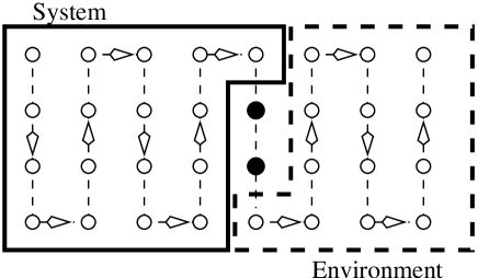
Figure 3: Schematic representation of the sweeping process in the standard DMRG method. The two black circles represent the probing sites which move throughout the 2D lattice onto the embedded dashed line which serves as a guide.

In two dimensions, the sweeping process is acomplished by embedding a one dimensional path into the whole lattice. This line is where the probing sites move along as the RG process proceeds.

In the PRG method the puncture can move through the lattice following several patterns. The most convenient is when each site is traversed 4 times in a cycle or sweep: left to right, right to left, up to down and down to up. This is graphically depicted in Fig. 4. Every sweep starts at the upper rightmost site and continues with a left movement towards the lower leftmost site of the lattice, following a zigzag line similar to that of the DMRG sweeping. At this moment the puncture comes back to the original site but following a down-to-up zigzag path. So far, each lattice site has been visited twice. To complete the sweeping cycle, there is another movement, this time with a up-to-down zigzag path, towards the lower leftmost site. Finally, the puncture comes back to the initial site with a zigzag down-to-up path.

Figure 4: Schematic representation of the sweeping process in the PRG method. Here the center of the plaquettes represent the actual sites of the real 2D lattice. Starting from the upper rightmost site, the lines indicate the successive steps executed to complete a whole cycle or sweeping.

Prior to the sweeping process, there is a warmup process to build up the finite lattice. There is no restriction about the initial data of the wave functions, but it is obvious that a smart guess shall boost the process. In the 1D and 2D cases we have prepared such a guess using a “Kadanoff-like” warmup: the original lattice is coarse-grained until the number of degrees of freedom is reduced to a given (small) value. Then the effective hamiltonian at this scale is exactly diagonalized and the resulting eigenfunctions are extrapolated to cover the whole original lattice.

In the 3D case we choose the initial data to be a gaussian random vector without correlation between different cells. Although it takes longer to achieve the desired precision, convergence is also completely fulfilled.

III Results in Several Dimensions

In this section we present our numerical results. We have made an extensive comparative analysis between the DMRG and the PRG involving different Hamiltonians, lattice’s size and dimensionality, number of states kept and number of punctures. We consider short-range and long-range interactions, in order to see whether the performance of the RG methods depends on this fact. We present our results in the following subsections according to the dimensionality of the lattices.

III.1 One-Dimensional Models

We have solved 3 types of potentials with the two RG methods:

Particle-in-a-box Potential: this is the free particle case, i.e. $V_{n}=0,\forall n$. The eigenfunctions are delocalized in real space.

Harmonic Oscillator: this is the standard quadratic potential $V_{n}=n^{2}$. The eigenfunctions are localized in the centre of the lattice.

2D Delta Potential: this model is a discretization, in momentum space, of the two-dimensional delta function potential delta . Due to the rotational symmetry the Hamiltonian is one-dimensional and it is given by

$$H_{nm}=\delta_{n,m}b^{2n}-g\;b^{n+m},\;\;M\leq n,m\leq N$$ (42)

where $n,m$ are momentum labels, $M$ and $N$ play the role of infrared and ultraviolet cutoffs, respectively, $b$ is a control parameter of the discretization which here we take as $b=\sqrt{2}$ and $g$ is the coupling constant of the delta function delta-g .

METHOD	PBOX		OSC		DELTA
	Sweeps	Time	Sweeps	Time	Sweeps	Time
Exact		$0.27$		0.26		$0.02$
DMRG	2	$0.36$	$2$	0.27	$4$	$1.5$
PRG (2)	65	$13.92$	$37$	7.69	$27$	$3.09$
PRG (4)	48	$4.75$	$25$	2.36	$10$	$1.25$
PRG (10)	34	$2.31$	$19$	1.25	$4$	$0.65$

Table 1: DMRG versus PRG numerical results for 1D systems. For all models $N_{E}=4$ and the number of sites is $N=100$ for PBOX and OSC, while $N=38$ for DELTA. The required precision is $10^{-10}$ for the GS and the first excited states. In the PRG method the number in parentheses represents the number of punctures $N_{p}$.

In Table I we present a summary of our numerical results. We have choosen the number of sweeps as the basic quantity to establish the comparison between the two RG methods. This is because this number only depends on the RG method employed for each model and not on the computer machine. However, to get an idea of what this number means we also give the corresponding computer time. Moreover, as it happens the time spent in a DMRG sweep is different than in a PRG sweep because the renormalization operations are also different. We have also solved these models using exact diagonalization techniques.

Table I shows that the number of sweeps needed by the DMRG to achieve the prescribed convergence ($10^{-10}$ for the $N_{E}/2$ lowest energy states) is much smaller than in the PRG method. This fact is independent of the model, the lattice size, the number of punctures $N_{p}$ and the number of targeted states $N_{E}$. We also observe that increasing the number of punctures lowers the number of PRG sweeps, which is nevertheless greater than the DMRG ones. On the other hand it is not reasonable to use a large number of punctures $N_{p}$, as compared to the total number of sites, for this amounts to an almost exact diagonalization of the model.

The bad convergence of the PRG method in 1D is due to the “rigidity” of the ansatz, meaning that the updates of the wave function affects in the same amount its left and right handed pieces. The high performance of the DMRG can be attributed to the “flexibility” of the ansatz, where the left and right handed pieces of the ansatz are updated independently.

III.2 Two-Dimensional Models

In two dimensions we have solved two models: the free particle and the Hydrogen atom whose Coulomb potential, in atomic units, takes the following form

$$V_{{\bf n}}=-\frac{2Z}{\sqrt{n_{1}^{2}+n_{2}^{2}}}$$ (43)

with $Z$ the atomic number which is fixed to 1. This problem is factorizable and admits an analytical solution in the continuum, with energies given by $E_{n}=-4Z^{2}/n^{2}$. We adopt a lattice discretization of (43) where the origin is placed at the centre of a plaquette.

METHOD	2D-HYDROGEN		2D-PBOX
	Sweeps	Time	Sweeps	Time
DMRG	9	$45.6$	$12$	65.7
PRG (1$\times$1)	15	$5.85$	$15$	5.85
PRG (2$\times$2)	5	$3.23$	$5$	3.22
PRG (3$\times$3)	3	$3.33$	$3$	3.32

Table 2: DMRG versus PRG numerical results for 2D systems. For all models $N_{E}=4$ and the number of sites is $N=10\times 10$ The required precision is $10^{-10}$ for the GS and first excited state. In the PRG method the number in parentheses represents the number of punctures $N_{p}$ (see Fig. 2).

In table II we display results for a $10\times 10$ lattice, which show that the PRG is more efficient than the DMRG. This fact is independent on the size of the lattice, the number of states kept and the model. The aforementioned “rigidity” of the PRG ansatz seems to be quite appropiate for 2D systems, while the left-right structure of the DMRG becomes a handicap.

The $N_{p}=4$ PRG reduces considerably the number of sweeps while the consumed (i.e. CPU) time is almost the same as for $N_{p}=9$. Both the number of sweeps and the CPU time for the PRG are quite insensitive to the model.

Figure 5: Log–log plot, time $t_{{\rm CPU}}$ versus length size $L$, for the 2D Hydrogen spectrum on a square lattice. Four states are targeted in each case, and a relative precision of $10^{-10}$ is required on the ground state and first excited state. The PRG uses a 2$\times$2 puncture as in Fig. 2.

In fig. 5 we plot the CPU time $t_{{\rm CPU}}$ versus the linear size of the square lattice $N_{1}=N_{2}\equiv L$ for the H-atom ( for the free particle we get similar results). From this plot we derive the scaling law

$$t_{{\rm CPU}}\propto L^{\theta}$$ (44)

Table III collects the numerical values of the exponent $\theta$ for the Exact, DMRG and PRG methods. They are the slopes of the curves in Fig. 5.

METHOD	PBOX	2D-HYDROGEN
Exact	$6.4\pm 0.3$	$6.61\pm 0.27$
DMRG	$5.5\pm 0.1$	$5.21\pm 0.05$
PRG	$3.92\pm 0.1$	$3.85\pm 0.07$

Table 3: Values of the exponent $\theta$ in (44) obtained with a linear fit of the data plotted in Fig. 5.

Fig. 5 shows that the elapsed time is always larger for the DMRG than for the PRG. Moreover, the $\theta$ exponent in the law (44) is also larger in the DMRG. This confirms that in 2D the PRG method is more efficient than the standard DMRG. Table III shows that this conclusion remains true for both types of models. For sufficiently large lattices the PRG performs better than the exact diagonalization methods.

As an illustration of how the PRG method works during the renormalization process leading to the determination of the lowest lying states of the models, we present in Figs. 7 and 8 a set of typical snapshots representing the four targeted wave functions in a 2D Hydrogen model and free particle. We do not plot the three dimensional picture of these wave functions, but instead the figure shows their projection onto the x-y plane, so that each grey square plaquette is more intense the higher the height (in absolute value) of the wave function. The punctures of the PRG method ($2\times 2$ and $1\times 1$) appear in these figures as blanck and white plaquettes respectively.

Making the superposition of all the screenshots of this sort, one for each of the RG-steps, one produces a movie showing the convergence process of the targeted wave functions starting from the warm-up initial states. During this “time” evolution one sees how the wave functions get shaped towards their final exact forms.

III.3 Three-Dimensional Models

We believe that the computations presented in one- and two-dimensional lattices are enough to make a thorough comparison of the two RG methods. However, we have also carried out calculations in three-dimensional lattices. The main purpose of this extension is to test the scaling laws obtained in the previous subsection for the PRG method. As far as the PRG version is concerned, there is no need for an extra effort in the computation and the sweeping process is a repetition of the one employed in two-dimensions, but traversing all the parallel planes making up the whole 3D lattice. However, we have not done the similar extension for the DMRG method for it was apparent from the previous subsection that the higher the dimensionality, the more unnatural the standard DMRG sweeping becomes. Thus, we expect a worse behaviour in the DMRG method as the dimension increases.

Figure 6: Same plot as Fig. 5, but for 3D Hydrogen atom. PRG is applied with a $2\times 2$ and a $3\times 3$ punctures. Notice the crossing between PRG lines and the exact ones.

We have chosen the three-dimensional Hydrogen atom as the representative model and thus, we have discretized the Coulomb potential

$$V_{{\bf n}}=-\frac{2Z}{\sqrt{n_{1}^{2}+n_{2}^{2}+n_{3}^{2}}}$$ (45)

with the proviso that the origin is placed outside the lattice, at the center of a cube, to avoid the singularity of the potential.

METHOD	3D-HYDROGEN
Exact	$9.51\pm 0.6$
PRG 2$\times$2	$6.6\pm 0.4$
PRG 3$\times$3	$5.6\pm 0.3$

Table 4: Values of the exponent $\theta$ in (44) obtained with a linear fit of the data plotted in Fig. 8.

Fig. 6 and table IV show that the $\theta$ exponents are larger than those in 2D. However, the 3D exponent for PRG is again lower than the corresponding one for the exact diagonalization method. In fact, the PRG exponent is not much larger than the DMRG exponent for 2D lattices. This fact makes us to believe that the PRG version is a well-behaved procedure in dimensions than one. Moreover, the fact that increasing the number of punctures reduces the number of sweeps is also reflected in this table by the smaller values of the $\theta$ exponent.

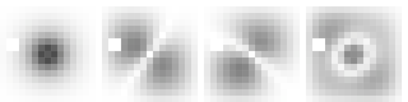
Figure 7: A typical screenshot of the PRG $2\times 2$ procedure for the 2D hydrogen atom on a $15\times 15$ square lattice and four target states. Notice the puncture near the upper–left corner. The puncture moves through the picture in a sweeping path, as depicted inf Fig. 4.

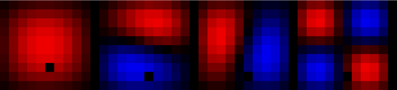
Figure 8: A typical screenshot of the PRG $1\times 1$ procedure for the 2D free particle on a $10\times 10$ square lattice and four target states. Notice the puncture as a black plaquette. The puncture moves through the picture in a sewing path, as depicted inf Fig. 4.

IV Conclusions and Prospects

In this paper we have explored the formulation of a single-block version of the DMRG method. The main motivation to undertake this study is the construction of a version of the DMRG which is better suited for higher dimensional lattices than the standard version.

We have stressed the role played by the sweeping process in the DMRG method and we have singled it out as one of the most relevant features of the finite-system formulation of the DMRG. It is this sweeping process what becomes one of the defining components of the PRG version of the DMRG and it is responsible for achieving the convergence of the lowest energy properties to a certain prescribed precision.

In 1D lattices the standard DMRG method outperforms the new PRG version. This is natural for we know that the DMRG is somehow optimal when dealing with one-dimensional models.

However, in 2D lattices the PRG formulation is more natural and well adapted to this type of lattices, unlike the DMRG which needs to split the lattice into left and right blocks. We have also tested numerically that the PRG gives a better performance than the DMRG for several types of models.

We have checked that the PRG method also perfoms well for 3D lattices. As a byproduct of this work, the PRG version can be considered as a new numerical method for solving the Schrödinger equation in 2D and 3D with a better efficiency than the exact diagonalization techniques, as can be seen from Tables III and IV.

Altogether we find these results quite promising, but of course the crucial issue is wether one can generalize the PRG to interacting many body systems. The technical point is to define a “puncture operation” of many body wave functions, which must isolate the “local” states associated with the puncture from the “global” states associated with the block. As we have shown in quantum mechanics this can be achieved by a set of local projection operators which “pick up” the value of the wave function at any given site ( see eq. 6). In the many body case one needs projection operators for all possible local states of the puncture. The formalism that is required to generalize the PRG to many body systems is reminiscent to the Matrix Product (MP) method progress . This fact may not be that surprising since after all the variational state underlying the DMRG is an inhomogenous MP ansatz.

- (1) S.R. White, Phys. Rev. Lett. 69, 2863 (1992).
- (2) S.R. White, Phys. Rev. B 48, 10345 (1993).
- (3) S.R. White and R. Noack, Phys. Rev. Lett. 68, 3487, (1992); R. Noack and S. White, Phys. Rev. B 47, 9243 (1993).
- (4) Density Matrix Renormalization, edited by I. Peschel, X. Wang, M. Kaulke and K. Hallberg (Series: Lecture Notes in Physics 528, Springer, Berlin, 1999).
- (5) S.R. White, Phys. Rep. 301 , 187 (1998).
- (6) K. Hallberg, “Density Matrix Renormalization”, CRM Proceedings (1999), Springer, Montreal (in press); cond-mat/9910082.
- (7) J. Gonzalez, M.A. Martin-Delgado, G. Sierra and A.H. Vozmediano, Quantum Electron Liquids and High- Superconductivity, chapter 11. Springer-Verlag: Monographs 38, Berlin Heidelberg (1995).
- (8) Strongly Correlated Magnetic and Superconducting Systems, eds. G.Sierra and M.A.Martin-Delgado, Lecture Notes in Physics 478, Springer Berlin, Heidelberg (1997)
- (9) S. R. White, R. M. Noack and D. J. Scalapino, Phys. Rev. Lett. 73, 886 (1994).
- (10) R. M. Noack, S. R. White and D. J. Scalapino, Phys. Rev. Lett. 73, 882 (1994); S. R. White, R. M. Noack and D. J. Scalapino, J. Low Temp. Phys. 99, 593 (1995); R. M. Noack, S. R. White and D. J. Scalapino, Europhys. Lett. 30, 163 (1995).
- (11) C. A. Hayward, D. Poilblanc, R. M. Noack, D. J. Scalapino and W. Hanke, Phys. Rev. Lett. 75, 926 (1995).
- (12) S.R. White, Phys. Rev. Lett. 77, 3633 (1996).
- (13) S.R. White and D.J. Scalapino, Phys. Rev. B 61, 6320 (2000).
- (14) S.R. White and D.J. Scalapino, Phys. Rev. B 60, R753 (1999).
- (15) S.R. White and D.J. Scalapino, Phys. Rev. Lett. 81, 3227 (1998).
- (16) H. B. Pang, H. Akhlaghpour and M. Jarrell, Phys. Rev. B 53, 5086 (1996).
- (17) T. Nishino, J. Phys. Soc. Jpn. 64, 3598 (1995).
- (18) T. Nishino and K. Okunishi, J. Phys. Soc. Jpn. 65, 891 (1996); ibid. 66, 3040 (1997); T. Nishino, K. Okunishi and M. Kikuchi, Phys. Lett. A 213, 69 (1996); T. Nishino and K. Okunishi, J. Phys. Soc. Jpn. 67, 3066 (1998).
- (19) T. Nishino, K. Okunishi, Density Matrix and Renormalization for Classical Lattice Models in Ref. elescorial (see also cond-mat/9610107).
- (20) K. Okunishi and T. Nishino, Prog. Theor. Phys. 103, 541 (2000).
- (21) T. Nishino, K. Okunishi, Y. Hieida, N. Maeshima and Y. Akutsu, Nucl. Phys. B575, 504 (2000).
- (22) S. Östlund and S. Rommer, Phys. Rev. Lett. 75, 3537 (1995).
- (23) M.A.Martin-Delgado and G. Sierra in Ref. dresden98 , Chap. 4, and references therein.
- (24) M.A. Martin-Delgado, J. Rodriguez-Laguna, G. Sierra. Nucl. Phys. B473, 685 (1996).
- (25) K.G. Wilson, Rev. Mod. Phys. 47, 773 (1975).
- (26) R. Noack and S. White in Ref. dresden98 , Chap. 2.
- (27) M.A. Martin-Delgado, G. Sierra and R.M. Noack, J. of Phys. A: Math. and Gen. 32, 6079 (1999).
- (28) M.A. Martin-Delgado and G. Sierra, Phys. Rev. Lett. 83, 1514 (1999).
- (29) The coupling constant is set to . This value of is choosen in such a way that the exact ground state energy of (42) is given exactly by delta .
- (30) Work in progress.