Metal-insulator transition in anisotropic systems

Abstract

We study the three-dimensional Anderson model of localization with anisotropic hopping, i.e., weakly coupled chains and weakly coupled planes. In our extensive numerical study we identify and characterize the metal-insulator transition by means of the transfer-matrix method and energy level statistics. Using high accuracy data for large system sizes we estimate the critical exponent as $\nu=1.6\pm 0.3$. This is in agreement with its value in the isotropic case and in other models of the orthogonal universality class.

Previous studies of Anderson localization And58 in three-dimensional (3D) disordered systems with anisotropic hopping using the transfer-matrix method (TMM) LiSEG89 ; ZamLES96a ; PanE94 , multifractal analysis (MFA) MilRS97 and energy-level statistics (ELS) MilR98 show that an MIT exists even for very strong anisotropy. In Refs. MilRS99a ; MilRSU00 , we studied critical properties of this second-order phase transition with high accuracy. Here we shall demonstrate the significance of irrelevant scaling exponents for an accurate determination of the critical disorder $W_{c}$ and the critical exponent $\nu$. Previous highly accurate TMM studies for isotropic systems of the orthogonal universality class reported $\nu=1.54\pm 0.08$ Mac94 , $\nu=1.58\pm 0.06$ SleO99a , $\nu=1.61\pm 0.07$, and $\nu=1.54\pm 0.03$ CaiRS99 , whereas for anisotropic systems of weakly coupled planes $\nu=1.3\pm 0.1$ and $\nu=1.3\pm 0.3$ was found ZamLES96a . We emphasize that this variation in theoretical values has its counterpart in the experiments where a large variation of $\nu$ has been reported with values ranging from 0.5 PaaT83 over 1.0 WafPL99 , 1.3 StuHLM93 , up to 1.6 BogSB99 . Possibly this experimental “exponent puzzle” StuHLM93 is due to other effects such as electron-electron interaction BogSB99 or sample inhomogeneities StuHLM93 ; RosTP94 ; StuHLM94 .

A further important aspect of anisotropic hopping besides the question of universality is the connection to experiments which use uniaxial stress, tuning disordered Si:P or Si:B systems across the MIT PaaT83 ; WafPL99 ; StuHLM93 ; BogSB99 . Applying stress reduces the distance between the atomic orbitals, the electronic motion becomes alleviated, and the system changes from insulating to metallic. Thus, although the explicit dependence of hopping strength on stress is material specific and in general not known, it is reasonable to relate uniaxial stress in a disordered system to an anisotropic Anderson model with increased hopping between neighboring planes.

We use the standard Anderson Hamiltonian And58

$${\bf H}=\sum_{i\neq j}t_{ij}|i\rangle\langle j|+\sum_{i}\epsilon_{i}|i\rangle\langle i|$$ (1)

with orthonormal states $|i\rangle$ corresponding to electrons located at sites $i=(x,y,z)$ of a regular cubic lattice with periodic boundary conditions. The potential energies $\epsilon_{i}$ are independent random numbers drawn uniformly from $[-W/2,W/2]$. The disorder strength $W$ specifies the amplitude of the fluctuations of the potential energy. The hopping integrals $t_{ij}$ are non-zero only for nearest neighbors and depend on the spatial directions, thus $t_{ij}$ can either be $t_{x}$, $t_{y}$ or $t_{z}$. We study (i) weakly coupled planes with $t_{x}=t_{y}=1$, $t_{z}=1-\gamma$ and (ii) weakly coupled chains with $t_{x}=t_{y}=1-\gamma$, $t_{z}=1$ with hopping anisotropy $\gamma\in[0,1]$. For $\gamma=0$ we recover the isotropic case, $\gamma=1$ corresponds to independent planes or chains. We note that uniaxial stress would be modeled by weakly coupled chains after renormalization of the hopping strengths such that the largest $t$ is set to $1$.

The MIT in the Anderson model of localization is expected to be a second-order phase transition BelK94 ; AbrALR79 . It is characterized by a divergent correlation length $\xi_{\infty}(W)\propto|W-W_{c}|^{-\nu}$ KraM93 . To construct the correlation length of the infinite system $\xi_{\infty}$ from finite size data $\xi_{M}$ ZamLES96a ; KraM93 ; PicS81a ; MacK81 , the one-parameter scaling hypothesis Tho74 $\xi_{M}=f(M/\xi_{\infty})$ is employed. One might determine $\nu$ from fitting to $\xi_{\infty}$ obtained by a FSS procedure MacK81 . Better accuracy can be achieved by fitting directly to the $\xi_{M}$ data Mac94 ; SleO99a ; CaiRS99 . We use fit functions SleO99a which include two kinds of corrections to scaling: (i) nonlinearities of the disorder dependence of the scaling variable and (ii) an irrelevant scaling variable with exponent $-y$ (cp. Fig. 1). For the nonlinear fit, we use the Levenberg-Marquardt method MilRS99a ; SleO99a . The input data $\xi_{M}$ for the FSS procedure are either (a) reduced localization lengths $\Lambda_{M}$ obtained by TMM with 0.07% accuracy and system widths up to $17\times 17$ for, e.g., the case of weakly coupled planes with $\gamma=0.9$ MilRSU00 ; or (b) integrated $\Delta_{3}$ statistics obtained from highly accurate ELS data (0.2% to 0.4%) and system sizes up to $50^{3}$ MilRS99a .

When applying the TMM to our anisotropic systems, one has to consider two non-equivalent orientations of the axis of the quasi-1D bar: parallel and perpendicular to the planes or chains. The localization lengths in the perpendicular direction are smaller than in the parallel direction by a factor of about $1-\gamma$ for coupled planes and $(1-\gamma)^{2}$ for chains ZamLES96a . The critical disorder $W_{c}$ should not depend on the orientation of the bar ZamLES96a . For strong anisotropies $\gamma\geq 0.9$ this is difficult to verify numerically due to strong finite size effects as shown in Fig. 1.

Figure 1: $\Lambda_{M}$ for coupled planes with $\gamma=0.9$ (perpendicular orientation) with relative error 0.1%, $W=7,\,7.1,\,7.2,\,\cdots,\,9.2$ and $M^{2}=5^{2},\,6^{2},\,7^{2},\,\cdots,\,22^{2}$. The solid lines in the right part are fits to the data with $y=2.05\pm 0.08$.

By computing data for very large system sizes up to $M^{2}=22^{2}$ ($46^{2}$) for the case of weakly coupled planes with $\gamma=0.9$ ($0.96$) we can show that this finite size effect can be sucessfully modelled (cp. Fig. 1) by an irrelevant scaling exponent and $W_{c}$ is indeed the same for both orientations.

In Fig. 2, we show fitted values obtained by FSS of TMM data for different choices of expansion coefficients in the nonlinear fit procedure. We conclude $\nu=1.62\pm 0.07$ and $W_{c}=8.63\pm 0.02$.

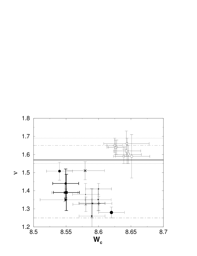
Figure 2: Results for $W_{c}$ and $\nu$, for coupled planes with $\gamma=0.9$, obtained from FSS of (parallel-direction) TMM data (open symbols) and ELS data. The error bars show the $95\%$ confidence intervals. The dotted (dashed) lines represent the error bounds for $\nu=1.62\pm 0.07$ ($1.45\pm 0.2$) of TMM (ELS). The solid line marks the result of SleO99a . The goodness of a fit is reflected in the size of the symbol. The $2$ thick error bars mark high quality ELS fits for large system sizes.

In Fig. 2, we also show the results for FSS of highly accurate ELS data (0.2% to 0.4%) and system sizes up to $N^{3}=50^{3}$. The error estimate is larger and the values of $W_{c}$ and $\nu$ are much more scattered than before. Comparing the spreading of the $W_{c}$ and $\nu$ values with their confidence intervals, the error estimates appear to be too small. E.g., the 95% confidence intervals of the smallest and largest $W_{c}$ value do not overlap. We therefore estimate $\nu=1.45\pm 0.2$ and $W_{c}=8.58\pm 0.06$ MilRS99a .

In conclusion, our results confirm the existence of an MIT for anisotropy $\gamma<1$ for weakly coupled planes found previsouly in studies using TMM ZamLES96a , MFA MilRS97 , and recently by ELS MilR98 . We have shown that large system sizes, high accuracies MilRS99a ; MilRSU00 and irrelevant scaling exponents are necessary to determine the critical behavior reliably. Our results are in good agreement with other high accuracy TMM studies for the orthogonal universality class Mac94 ; SleO99a ; CaiRS99 ; SleO97 . These numerical estimates seem to converge towards $\nu\approx 1.6$.

- (1) P. W. Anderson, Phys. Rev. 109, 1492 (1958).
- (2) Q. Li, et al., Phys. Rev. B 40, 2825 (1989).
- (3) I. Zambetaki, et al., Phys. Rev. Lett. 76, 3614 (1996).
- (4) N. A. Panagiotides, S. N. Evangelou, and G. Theodorou, Phys. Rev. B 49, 14122 (1994).
- (5) F. Milde, R. A. Römer, and M. Schreiber, Phys. Rev. B 55, 9463 (1997).
- (6) F. Milde and R. A. Römer, Ann. Phys. (Leipzig) 7, 452 (1998).
- (7) F. Milde, R. A. Römer, and M. Schreiber, Phys. Rev. B 61, 6028 (2000), cond-mat/9909210.
- (8) F. Milde, R. A. Römer, M. Schreiber, and V. Uski, Eur. Phys. J. B 15, 685 (2000), cond-mat/9911029.
- (9) A. MacKinnon, J. Phys.: Condens. Matter 6, 2511 (1994).
- (10) K. Slevin and T. Ohtsuki, Phys. Rev. Lett. 82, 382 (1999), cond-mat/9812065.
- (11) P. Cain, R. A. Römer, and M. Schreiber, Ann. Phys. (Leipzig) 8, SI33 (1999), cond-mat/9908255.
- (12) M. A. Paalanen and G. A. Thomas, Helv. Phys. Acta 56, 27 (1983).
- (13) S. Waffenschmidt, C. Pfleiderer, and H. v. Löhneysen, Phys. Rev. Lett. 83, 3005 (1999), cond-mat/9905297.
- (14) H. Stupp et al., Phys. Rev. Lett. 71, 2634 (1993).
- (15) S. Bogdanovich, M. P. Sarachik, and R. N. Bhatt, Phys. Rev. Lett. 82, 137 (1999).
- (16) T. F. Rosenbaum, G. A. Thomas, and M. A. Paalanen, Phys. Rev. Lett. 72, 2121 (1994).
- (17) H. Stupp et al., Phys. Rev. Lett. 72, 2122 (1994).
- (18) D. Belitz and T. R. Kirkpatrick, Rev. Mod. Phys. 66, 261 (1994).
- (19) E. Abrahams, et al., Phys. Rev. Lett. 42, 673 (1979).
- (20) B. Kramer and A. MacKinnon, Rep. Prog. Phys. 56, 1469 (1993).
- (21) J.-L. Pichard and G. Sarma, J. Phys. C: 14, L127 (1981).
- (22) A. MacKinnon and B. Kramer, Phys. Rev. Lett. 47, 1546 (1981); Z. Phys. B 53, 1 (1983).
- (23) D. J. Thouless, Phys. Rep. 13, 93 (1974).
- (24) K. Slevin and T. Ohtsuki, Phys. Rev. Lett. 78, 4083 (1997), cond-mat/9704192.