Tribology and hardness Interface structure and roughness Elasticity, fracture and flow

Elastic Response of Rough Surfaces in Partial Contact

Abstract

We model numerically the partial normal contact of two elastic rough surfaces with highly correlated asperities. Facing surfaces are unmated and described as self-affine with a Hurst exponent $H$. The numerical algorithm is based on Fourier acceleration and allows efficient simulation of very large systems. The force, $F$, versus contact area, $A$, characteristics follows the law $F\sim A^{(1+H)/2}$ in accordance with the suggestion of Roux et al. (Europhys. Lett. 23, 277 (1993)). However finite size corrections are very large even for $512\times 512$ systems where the effective exponent is still 20% larger than its asymptotic value.

The mechanical properties of bodies in contact have been studied for a long time [1] since they have important applications ranging from the flow properties of powders to earthquake dynamics [2]. For example, frictional properties are related to the normal stresses that develop during contact, and they have recently been shown to be very sensitive to heterogeneities in the normal stresses [3]. On the fault scale, the dynamical stress field, which is responsible for earthquakes, is strongly influenced by heterogeneities due to asperity squeeze [4].

In this letter we investigate numerically the elastic response of self-affine rough surfaces that are squeezed together. The rough surface, which we take to be oriented in the $(x,y)$ plane, is given by $z=z(x,y)$. If $p(z;x,y)$ is the probability density to find the surface at a height $z$ at $(x,y)$, self affinity is the scaling property

$$\lambda^{H}p(\lambda^{H}z;\lambda x,\lambda y)=p(z;x,y)\;,$$ (1)

where $H$ is the Hurst or roughness exponent [5, 6]. There is strong experimental evidence that surfaces resulting from brittle fracture are self affine with a Hurst exponent equal to $0.8$ [7, 8, 9, 10, 11, 12].

When two elastic media are forced into contact along two non-matching self-affine rough surfaces, two mechanisms conspire to produce a power law dependence of the applied normal force $F$ on the penetration depth, $D$: (1) the contact area increases as $D$ is increased, and (2) the fluctuations in the normal stress field where there is contact reflect the self affinity of surfaces. In the much simpler case of a spherical asperity in contact, Hertz showed about 120 years ago [13] that $F\sim D^{3/2}$, and $A\sim D$. The Hertz law has been verified experimentally in the case of a diamond stylus sliding on a diamond surface [14]. The power law dependence of the force on penetration has also been established experimentally for fracture surfaces in contact [15].

In 1993, Roux et al. [16] proposed the following dependence of $F$ and $A$ on $D$ for self-affine elastic surfaces in contact,

$$F\sim D^{1+1/H}\;,$$ (2)

and

$$A\sim D^{2/H}\;,$$ (3)

where $H$ is the smallest Hurst exponent of the two surfaces. The argument goes as follows. First, we note that the rough surface with the smallest Hurst exponent is the roughest and will dominate the scaling properties of the common interface of the two media in contact up to a cross-over length scale [17]. Second, we note that nowhere in the arguments that follow will we need both surfaces to deform. Thus, we will make the assumption that the surface with the largest Hurst exponent (or one of them if they have the same Hurst exponent) simply is flat and elastic, whereas the other one is rough and infinitely rigid. Let us now rescale the spatial coordinates of the surface, $x\to\lambda x$, $y\to\lambda y$ and $z\to\lambda^{H}z$. As a consequence of Eq. (1), the surface is statistically invariant under this operation. The penetration $D$ needs to be rescaled $D\to\lambda^{H}D$ as it “points” in the $z$ direction, and the contact area $A\to\lambda^{2}A$ as it lies in the $(x,y)$ plane. The local deformation, $u$, of the surface must be rescaled as $u\to\lambda^{H}u$, since $u$ also “points” in the $z$ direction. The local deformation, $u$, at $(x,y)$ is related to the normal stress field $\sigma$ by the expression [13]

$$u(x,y)=\int\int dxdyG(x-x^{\prime},y-y^{\prime})\sigma(x^{\prime},y^{\prime})\;,$$ (4)

where $G\sim 1/r$, and $r=|(x-x^{\prime},y-y^{\prime})|$. Thus, we find that $\sigma\to\lambda^{H-1}\sigma$ under rescaling [18]. The total force $F=A\sigma$, and consequently, $F\to\lambda^{1+H}F$ under rescaling. Eliminating $\lambda$ between any pair of variables in the above expressions, gives the power law dependence of the different variables. In particular, we find Eqs. (2) and (3) and

$$F\sim A^{(1+H)/2}\;.$$ (5)

Eq. (2) was tested experimentally and numerically in Ref. [19]. The obtained results were consistent with the suggestions of Roux et al. [16], but hardly convincing. The first problem was that the definition of the zero level of the penetration is not the point of first contact between the two surfaces, but rather has to be treated as a free parameter in the data fits. Another numerical problem encountered was the necessity to invert dense matrices, with the consequence that only small systems could be studied (up to $32\times 32$).

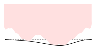
Figure 1: A stiff medium with a rough surface (top) is pushed into an elastic, flat medium (bottom). The dashed, horizontal line represents the undeformed medium at a given penetration depth, while the full line represents the actual surface of the medium. The penetration depth $D$ is defined with respect to the dashed line.

In the present letter, we have developed a new and much more efficient algorithm that allows us to simulate easily systems up to $512\times 512$. We are, therefore, able to present convincing tests of the scaling relation Eq. (5). Whereas the numerics of Ref. [19] were based on six samples of size $32\times 32$, we base our data on $300$ samples of size $512\times 512$. One surprising result in the present study is how strong the finite-size corrections to the results are. Size is estimated in units of the lower cut-off scale for the self-affine invariance of the rough surfaces.

We now describe the model and its numerical solution. We represent both surfaces on two-dimensional $L\times L$ lattices with deformations taking place only in the third transverse direction. The discretization size is adjusted to the unit size that is the lower cut-off length of the self-affine scaling. As the hard rough surface is pushed into the elastic one, the forces and deformations are described by the discrete version of Eq. (6),

$$u_{i}=\sum_{j}G_{i,j}f_{j}\;,$$ (6)

with the Green function given by

$$G_{i,j}={{2(1-s)(1+s)}\over{2\pi e\ |{\vec{i}}-{\vec{j}}|}}\;.$$ (7)

$u_{i}$ is the deformation of the elastic body at site $i$ and $f_{i}$ the force acting at that point. In the Green function, $s$ is the Poisson ratio, $e$ the elastic constant, and $|{\vec{i}}-{\vec{j}}|$ the distance between sites $i$ and $j$. The indices $i$ and $j$ run over all $L^{2}$ sites.

To define the problem completely, the boundary conditions need to be specified. Clearly, in the regions where the rough surface is in contact with the elastic one, the deformation, $u_{i}$, is specified (it conforms to the shape of the rough surface) and one solves for the force. On the other hand, in the regions where contact has not been established, the elastic surface deforms in response to the influences from the contact regions. In this case equilibrium is established when the net forces acting on the surface vanish. Therefore, in the no-contact region, the force is specified, it vanishes, and one solves for the deformation.

We can build these boundary conditions into the equations to facilitate solving them. To do this, we define the diagonal $L^{2}\times L^{2}$ matrix, ${\bf K}$, with elements equal to $1$ on contact sites and $0$ on free (no-contact) sites. Clearly the vector ${\bf K}{\vec{u}}$ is zero everywhere there is no contact. At contact points, ${\bf K}{\vec{u}}$ is equal to the imposed deformation given by the shape of the rough surface.

Eq. (6) can be rewritten as,

$${\bf G}({\bf I}-{\bf K}){\vec{f}}+{\bf G}{\bf K}{\vec{f}}=({\bf I}-{\bf K}){\vec{u}}+{\bf K}{\vec{u}}\;,$$ (8)

where we use matrix-vector notation, and ${\bf I}$ is the identity. This form is convenient because as mentioned above, ${\bf K}{\vec{u}}$ is a known quantity (boundary condition). In addition, the vector $({\bf I}-{\bf K}){\vec{f}}$ is always zero because the force ${\vec{f}}$ is nonzero only at contact points. Putting the unknowns on the left hand side and the boundary conditions on the right hand side of Eq. (8) we obtain,

$${\bf G}{\bf K}{\vec{f}}-({\bf I}-{\bf K}){\vec{u}}={\bf K}{\vec{u}}\;.$$ (9)

Now define the vector ${\vec{x}}$ representing all the unknown quantities. Clearly,

$${\vec{x}}={\bf K}{\vec{f}}+({\bf I}-{\bf K}){\vec{u}}\;.$$ (10)

With this definition, and noting that ${\bf K}({\bf I}-{\bf K})=({\bf I}-{\bf K}){\bf K}=0$, ${\bf K}^{2}={\bf K}$, and $({\bf I}-{\bf K})^{2}=({\bf I}-{\bf K})$ we can write Eq. (9) as

$${\bf G}{\bf K}{\vec{x}}-({\bf I}-{\bf K}){\vec{x}}={\bf K}{\vec{u}}\;,$$ (11)

and finally

$$\bigl{(}{\bf I}-({\bf I}-{\bf G}){\bf K}\bigr{)}{\vec{x}}={\bf K}{\vec{u}}\;.$$ (12)

Eq. (12) is of the familiar form, ${\bf A}{\vec{x}}={\vec{b}}$ which can be solved using, for example, the Conjugate Gradient (CG) method [20, 21]. The difficulty is that the Green function ${\bf G}$ is represented by a full $L^{2}\times L^{2}$ matrix. This will lead to the number of operations per iteration scaling as $L^{4}$ which is prohibitive. We overcome this difficulty by doing the matrix multiplications involving ${\bf G}$ in Fourier space by using FFTs. This leads to a stable and extremely efficient algorithm, scaling like $L^{2}\ln(L)$, with which we were able to study systems with size up to $L=512$.

One more technical detail remains. The matrix ${\bf K}$, which indicates the contact points needs to be determined. The problem is that as we push the rough surface into the elastic one, the latter deforms. Therefore, the contact area is not equal to the area obtained by simply taking a cut through the rough surface. We obtain the correct contact area as follows. Our initial assumption is that the contact area is equal to the area obtained from a simple cut of the rough terrain, see Fig. 1. This determines the initial ${\bf K}$ which is then used in Eq. (12). The solution thus obtained gives the forces where there is contact and the deformations where there is none. Some of the forces thus obtained are negative since the elastic surface is trying to pull away from the rough surface. We therefore modify ${\bf K}$ by zeroing the elements corresponding to sites where the force is negative, and we solve again. We repeat this process until there are no sites with negative forces. This algorithm always converges giving the correct contact area and forces.

Figure 2: Contact area versus force for a hard sphere with radius $R=6000$ squeezed into an elastic flat medium with elastic constant $e=100$ (i.e. a Hertz contact). The calculation is done on a $512\times 512$ lattice. The least-squares fit, assuming a power law gives $A\sim F^{0.63}$.

To verify the algorithm and program we first tested it with a Hertz contact. Figure 2 shows the force-contact area characteristics of a hard sphere with radius $R=6000$ which is pushed into an elastic, flat medium with elastic constant $e=100$. The calculation was done on a $512\times 512$ lattice. The exact Hertz solution gives $A\sim F^{2/3}$, while a least-squares fit on the data gives $A\sim F^{0.63}$. The exponent given by our model, $0.63$, is in excellent agreement with the exact value, the difference being due to finite size effects. We have verified that for smaller systems and smaller asperities, the exponent moves farther away from the $2/3$ value.

Having established that the algorithm works correctly, we then simulated various aspects of squeezing a stiff self-affine surface into an initially flat elastic one. We measured the total force, $F$, as a function of the total contact area, $A$. In addition, for all situations simulated, we measured the force at each contact point thus obtaining a very detailed picture of the squeezing process.

Figure 3: left: Force, $F$, versus contact area, $A$, for 300 independent samples of hard self-affine surfaces with $H=0.8$ pushed into an initially flat medium with elastic constant $e=100$. System sizes from bottom to top: $32$, $64$, $128$, $256$ and $512$. right: Same but with $H=0.6$ and sizes up to $256$.

We show in Fig. 3 the force, $F$, versus contact area, $A$, for different system sizes and Hurst exponent $H=0.6,0.8$. The data are averaged over $300$ samples for each size and $H$. The elastic constant for the elastic, flat medium is $e=100$. Even though the force versus contact area curves produce very high-quality fits to power laws, $F\sim A^{\alpha}$, the resulting exponents, $\alpha$, depend strongly on the system size, $L$, even for systems as large as $512\times 512$. For $H=0.8$, we find from Fig. 3, $\alpha(L=32)=1.33$, $\alpha(64)=1.27$, $\alpha(128)=1.21$, $\alpha(256)=1.16$, and $\alpha(512)=1.12$. Correspondingly, from Fig. 3, we find for $H=0.6$, $\alpha(L=32)=1.31$, $\alpha(64)=1.24$, $\alpha(128)=1.19$, and $\alpha(256)=1.13$.

In figure 4 we show these exponents versus $1/L^{b}$ for $H=0.8$ (circles) and $H=0.6$ (triangles). It is clear from this figure that the finite size effects are large. It is not easy to extrapolate to $L\to\infty$ using $\alpha(L)=\alpha_{\infty}+aL^{-b}$ because the power law has a small exponent, $b$, and requires much larger sizes to give reasonable results to this three parameter fit. Instead, we will verify the result of reference [16] by fitting to a one parameter function, $\alpha(L)=(1+H)/2+L^{-b}$. The results are shown as solid lines in Fig. 4. The high quality of the fits strongly supports the result $\alpha_{\infty}=(1+H)/2$. We found $b=0.24$ for $H=0.8$ and $b=0.2$ for $H=0.6$. It is not clear if the difference between the two exponents is meaningful.

Figure 4: Effective exponent $\alpha$ versus $1/L^{b}$, where $L$ is the system size. Circles are for $H=0.8$ and give $b=0.24$, triangles are $H=0.6$ and give $b=0.2$. Curves are given by $\alpha=(1+H)/2+L^{-b}$.

It is worth noting that although the case of the Hertz contact did display some finite size effects, they were very small especially when compared with the large effects observed with self affine surfaces. This can be attributed to the long distance correlations in self affine surfaces.

Thanks to a fast algorithm based on Fourier acceleration we were able to describe precisely the evolution of the contact between two elastic rough surfaces from the first contact of one asperity to the maximum contact (see below). Asperity roughness is characterized by a self-affine (Hurst) exponent in a range compatible with fractured surfaces. Our algorithm easily allows extension to other roughness exponents. We demonstrated that the theoretical prediction from Roux et al [16] is valid but very strong finite size effects exist. For instance, the effective relationship between normal force and contact area is

$$F\propto A^{(1+H)/2+L^{-b}}$$ (13)

were $b\approx 0.2$. This finite size effect results in a large sensitivity to the cut-off scale of the self-affine scaling.

Finally, we remark that when we push a hard rough body into the elastic initially flat one, the maximum contact area, $A/L^{2}$, obtained is never unity! In Fig. 3 we show the total force, $F$, versus the contact area, $A/L^{2}$, up to the maximum attainable contact area. It is clear from the figure that it is not unity: For the $L=512$ system it is of the order of $20\%$. If we allow plastic yield, full contact would be attainable. This is straightforward to do in our model.

- [1] K. L. Johnson, Contact Mechanics (Cambridge University Press, Cambridge, 1985).
- [2] C. H. Scholz, The Mechanics of Earthquakes and Faulting (Cambridge Univ. Press, Cambridge, 1990).
- [3] J. Dieterich and B. Kilgore, Tectonophysics, 256, 216 (1996).
- [4] M. Bouchon, M. Campillo and F. Cotton, J. Geophys. Res. 103, 21091 (1998).
- [5] J. Feder, Fractals (Plenum Press, New York, 1988).
- [6] A. L. Barabási and H. E. Stanley, Fractal Concepts in Surface Growth (Cambridge University Press, Cambridge, 1997).
- [7] S. R. Brown and C. H. Scholz,J. Geophys. Res. 90, 12575 (1985).
- [8] W. L. Power, T. E. Tullis, S. R. Brown, G. N. Boitnott and C. H. Scholz, Geophys. Res. Lett. 14, 29 (1987).
- [9] E. Bouchaud, G. Lapasset and J. Planès, Europhys. Lett. 13, 73 (1990).
- [10] K. J. Måløy, A. Hansen, E. L. Hinrichsen and S. Roux, Phys. Rev. Lett. bf 68, 213 (1992).
- [11] J. Schmittbuhl, F. Schmitt and C. H. Scholz, J. Geophys. Res. 100, 5953 (1995).
- [12] E. Bouchaud, J. Phys.: Condens. Matter 9, 4319 (1997).
- [13] L. Landau and E. Lifshitz, Theory of Elasticity (Pergamon Press, Oxford, 1958).
- [14] F. P. Bowden and D. Tabor, The friction and Lubrication of Solids. Part II., Clarenden Press, Oxford, 1964.
- [15] J. T. Oden and J. A. C. Martins, Comput. Methods Appl. Mech. 52, 527 (1985).
- [16] S. Roux, J. Schmittbuhl, J. P. Vilotte and A. Hansen, Europhys. Lett. 23, 277 (1993).
- [17] F. Plouraboué, P. Kurowski, J. P. Hulin, S. Roux, and J. Schmittbuhl, Phys. Rev. E 51, 1675 (1995).
- [18] A. Hansen, J. Schmittbuhl, G. G. Batrouni, and F. di Oliveira, Geophys. Res. Lett., in press.
- [19] K. J. Måløy, X. L. Wu, A. Hansen and S. Roux, Europhys. Lett. 24, 35 (1993).
- [20] W. H. Press, S. A. Teukolsky, W. T. Vetterling and B. P. Flannery, Numerical Recipes in Fortran 77: The Art of Scientific Computing (Cambridge University Press, Cambridge, 1992).
- [21] G. G. Batrouni and A. Hansen, J. Stat. Phys. 52, 747 (1988).