Renormalization Group and Perfect Operators for Stochastic Differential Equations

Abstract

We develop renormalization group (RG) methods for solving partial and stochastic differential equations on coarse meshes. RG transformations are used to calculate the precise effect of small scale dynamics on the dynamics at the mesh size. The fixed point of these transformations yields a perfect operator — an exact representation of physical observables on the mesh scale with minimal lattice artifacts. We apply the formalism to simple nonlinear models of critical dynamics, and show how the method leads to an improvement in the computational performance of Monte Carlo methods.

PACS Numbers: 05.10.Cc, 05.10.-a, 05.10.Ln, 64.60.Ht

I Introduction

The purpose of this paper is to introduce numerical methods that avoid unnecessary discretization — or, over-discretization — purely for the purpose of obtaining adequate accuracy. An important and classical example of this is large eddy simulation in the modeling of turbulent flows. Many large scale flows of engineering, geophysical or atmospheric interest contain many length scales down to the dissipation scale, yet it is large scale drag that one wants to compute. In such a situation, it is wasteful and undesirable to expend computer time on details that are of no intrinsic interest.

The approach outlined in this paper builds upon our previous work[1] to use RG methods to integrate out the dynamics one wishes to ignore, so that numerical methods can instead focus on the appropriate scale of interest. This is not trivial because of scale interference: the nonlinear amplification of the effect of small scale dynamics, which contaminates and eventually pollutes the large scale dynamics. There are several distinct facets to this problem.

First is the representation of the small scale dynamics as a stochastic field that acts on the coarse-grained degrees of freedom. As discussed in our earlier paper, this inevitably leads to non-locality. We will see here that it is possible not only to coarse-grain individual operators, as in ref. [1] but also to coarse-grain at the level of the governing differential equation. This leads to a theory that is non-local in space and time. This applies to systems with a finite number of degrees of freedom, as well as spatially extended systems, which are the main focus of our work here.

Second, the representation of the theory on the lattice can be improved by systematically integrating out the small scales, leading to an effective theory that has no (or few) residual discretization artifacts. This is referred to as a “perfect theory” in the literature. We demonstrate how this arises and exhibit this feature by calculating the dispersion relation of the effective theory in the perfect representation.

Our work is related to that of Chorin and co-workers [2, 3, 4, 5, 6] who use optimal prediction methods to treat the lack of resolution of small scales. The main differences are that they assume that the small scales are initially in thermal equilibrium, and also that they do not attempt to remove lattice artifacts. There has also been an attempt to use similar methods in the study of isotropic turbulence[7].

Our work grew out of attempts to improve lattice gauge theory, pioneered by the paper of Hasenfratz and Niedermeyer. For a review of this body of work, the reader is referred to the review article by Hasenfratz[8]. In addition to the work in ref. [1], there have been two attempts[9, 10] to solve differential equations using perfect operators. As we will see below, it is not enough to perfectly coarse-grain the individual operators appearing in a partial differential equation: once there is a non-infinitesimal time step, coarse-graining introduces memory effects, so that the entire differential equation must be represented as coarse-grained in space-time. In addition, it should always be remembered that there is no unique perfect operator for a given differential operator. A specification must be made of the microscopic probability distribution for the small-scale degrees of freedom. These papers implicitly impose a Gaussian free field theory distribution on the small-scale degrees of freedom. The methods given in the present article are more general, and make no such assumption, explicit or implicit.

Let us now introduce the problem of removing lattice artifacts. Suppose the dynamics of a spatially extended system is described by a partial differential equation (PDE), which yields the solution $u(x,t)$. A standard procedure is to sample $u(x,t)$ at points ${x_{i},t_{j}}$, which are equidistant with spacings $\Delta x$ and $\Delta t$, and find a discretized form of the PDE that is devised to approximate the values $u_{i,j}\equiv u(x_{i},t_{j})$. The requirement is that in the continuum limit, the sequence $u_{i,j}$ converges to $u(x,t)$. The conventional way of discretizing the PDE is to approximate differentiations with finite differences.

The disadvantage of this uniform sampling (US) approach is that one is forced to reproduce as faithfully as possible all the detail and fine structure of the solution, even on a scale that may be of no interest or worse, beyond the regime of applicability of the differential equation itself. This has two consequences:

• a small grid size $\Delta x$ must be used, which implies many grid points must be calculated and stored;

• for dynamic problems, a small time step $\Delta t$ is implied by the small $\Delta x$, either for reasons of accuracy or stability of the numerical method.

As a result, there is a huge computational cost associated with this conventional numerical scheme, which makes the study of problems such as critical dynamics and pattern formation very difficult to carry out. There is a need for improved, physically motivated methods for numerical experiments.

The purpose of a numerical simulation is to study the macroscopic properties of a physical system. Different microscopic dynamics may be related, via coarse graining (CG), to the same macroscopic dynamics that defines a universality class. Often CG means the local averaging of a continuous variable,

$$U(X)=\int^{\Lambda/2}_{-\Lambda/2}dx\,u(X+x)\,,$$ (1)

where $u(x)$ is the continuum variable, $U(X)$ is its coarse-grained counterpart and $\Lambda$ is the coarse graining length scale. Instead of focusing on the small scale degrees of freedom, we should determine and use the coarse grained description of the system appropriate at the macroscopic scale.

One of these physics-motivated numerical methods is the cell dynamical scheme[11], in which a discrete description of the system dynamics is obtained directly from considerations of the underlying symmetry and conservation laws. It has been successfully used to tackle problems such as asymptotic scaling behavior in spinodal decomposition[12] and the approach to equilibrium in systems with continuous symmetries, such as XY magnets[13] and liquid crystals[14]. There have also been attempts at using the RG in dynamic Monte Carlo simulations[15, 16].

To investigate what is required to obtain a coarse-grained dynamic description, suppose that we denote the coarse-graining operator at scale $\Lambda$ by the symbol $C_{\Lambda}$, which transforms $u(x,t)$ to $U(X,t)$. Then conceptually we need to find the operator $L_{\Lambda}$ which connects $U(X,0)$ and $U(X,t)$ given the microscopic time evolution operator $L$ connecting $u(x,0)$ with $u(x,t)$, as shown schematically in the commutativity diagram below:

$$u(x,0) \quad\mathop{\longrightarrow}\limits^{L}\quad u(x,t)$$

$$C_{\Lambda}\Bigg{\downarrow} C_{\Lambda}\Bigg{\downarrow}$$

$$U_{\Lambda}(X,0) \quad\mathop{\longrightarrow}\limits^{L_{\Lambda}}\quad U_{\Lambda}(X,t)$$

Notice that there is not a unique choice of $C_{\Lambda}$. The usual choice is local averaging. In principle, other operators can be used, such as the majority rule scheme used in the coarse graining of Ising spins in thermal equilibrium. Once a coarse-graining operator $C_{\Lambda}$ has been defined, there should be a unique prescription to obtain $L_{\Lambda}$[17]. In this paper, coarse graining is understood to mean local averaging. Later, stochastic coarse graining will be introduced as a variant of the simple local averaging. In the development of the theory of perfect operators a parameter, denoted here by $\kappa_{0}$ (see section IIIB), naturally arises, which characterizes the nature of the coarse-graining procedure. The form (1) is only appropriate if $\kappa_{0}$ is infinite; if $\kappa_{0}<\infty$, additional noise terms are generated which reflect the reduction in the number of degrees of freedom in the system. As already stressed in our earlier paper[1], it is inconsistent to work with a perfect operator with $\kappa_{0}<\infty$ and to use the $\kappa_{0}=\infty$ form (1) as some authors[9, 10] have done. We also see no reason why coarse-grained equations should be derived by varying a coarse-grained action in the absense of a small parameter, which is the starting point of these authors. Instead we begin with a dynamics which is intrinsically stochastic and study the effect of CG on this system. The well-known path-integral formulation of such equations may then be used to carry out the CG: there is no need to invoke a variational principle.

We need to consider the appropriate coarse-graining scale. Two situations are possible here. In the first, we suppose that the solution we wish to obtain has a natural scale $\Lambda$ below which there is no significant structure. In that case, our goal is to avoid having to over-discretize the problem merely in order to attain the accuracy of the continuum limit. Thus, we would like to be able to use as large a value for the grid spacing $\Delta x$ as possible without sacrificing accuracy. In the second situation, there is no such obvious scale, or at least, it is not known a priori, but the computational demands are so large that it is simply not feasible to work with a grid spacing $\Delta x$ smaller than some size $\Lambda$. In this case, we would like to minimize in some sense the artifacts that must inevitably arise.

The first situation is more straightforward because the only issue is speed of convergence to the continuum limit: there is no explicit discarding of important dynamical information. In the second situation, one is making an uncontrolled and potentially severe truncation of the correct dynamics. One has to ask: can one model the neglected unresolved scales as effective renormalizations of the coefficients in the original PDE? Are the neglected degrees of freedom usefully thought of as noise for the retained large-scale degrees of freedom? And how can any available statistical information on the small-scale degrees of freedom be used to improve the numerical solution for the large-scale degrees of freedom?

The plan of the paper is as follows. In section II we set up the coarse-graining algebra, which forms the basis of our approach, using the path-integral formulation of stochastic dynamics as our starting point. This formalism is then used in section III to obtain the perfect operator for dynamics governed by linear operators. Section IV describes the results of numerical simulations using the perfect operator with Langevin dynamics and section V using the Monte Carlo approach. A range of issues is discussed, from applications of the method to the diffusion equation and nonlinear model A dynamics to the question of the truncation of perfect operators required when carrying out simulations. Our conclusions are presented in section VI and the structure of the coarse-graining algebra is discussed in an appendix.

II Coarse Graining in the Path Integral Formulation of Langevin Dynamics

In this section, we derive the path integral formulation of the Langevin dynamics and present the general framework under which the perfect linear operator is derived. The analysis is applicable to both PDEs and stochastic differential equations. For simplicity, we study a system whose dynamics is described by a stochastic differential equation (SDE) with the following form,

$$\frac{\partial\phi(x,t)}{\partial t}=-f(x,t;\{\phi\})+\eta(x,t)\,,$$ (2)

where $\phi$ is a field, $f$ is the forcing term (it can depend on $\phi$ and/or its spatial derivatives), and $\eta$ is a white noise.

It is convenient to regularize the problem on a (fine) $N\times N^{\prime}$ lattice with grid size $\Delta x$ and $\Delta t$ in the space and time directions, respectively. In the lattice picture, all variables in the original PDE are vectors of functions of discrete space $x=i\Delta x$ and time $t=j\Delta t$ where $i\in[0,N-1]$, $j\in[0,N^{\prime}-1]$. We define $g(i\Delta x,j\Delta t)\equiv g(i,j)$ and denote the space-time volume element $\Delta x\Delta t$ by $\Delta V$. The noise satisfies $\langle\eta(i,j)\rangle=0$ and $\langle\eta(i,j)\,\eta(i^{\prime},j^{\prime})\rangle=\frac{\Omega}{\Delta V}\,\delta_{i,j}\,\delta_{i^{\prime},j^{\prime}}$ where $\Omega$ is the noise strength and $\delta_{i,j}$ is the Kronecker symbol. Given the system is in the state $\phi_{0}$ at time $t_{0}$, the probability that the system will be in state $\phi_{1}$ at time $t_{1}$ is given by[18],

$$P(\phi_{1},t_{1}|\phi_{0},t_{0})=\int D\phi\,D\eta\,\exp\{-\frac{\Delta V}{2\Omega}\sum^{N,N^{\prime}}_{i,j}[\eta^{2}(i,j)-\frac{\Omega}{\Delta x}\partial_{\phi}f]\}\,\delta(\eta-\partial_{t}{\phi}-f(\phi))\,,$$ (3)

where the integration is over all configurations beginning at $\phi_{0}$ and ending at $\phi_{1}$. We can use this path-integral formula to determine the dynamics followed by the coarse grained or uniform sampled variable.

By a discretization scheme, we will mean a process made up of a series of magnifying operations which lead from a microscopic description of a system to a macroscopic description on a lattice. These magnification operations are, by default, magnification of a length scale by a factor of 2. Coarse graining and uniform sampling are both special cases of a discretization scheme.

Suppose a system is specified by the values of a function $f$, such as a field configuration, on a fine lattice with 2N grid points $x=(x_{1},x_{2},\cdots,x_{2N})$ separated by grid size $\Delta x$. One step (level) of coarse graining is defined as local averaging of the function’s values at every two neighboring sites.

$$\bar{f}_{n}=\frac{1}{2}(f_{2n-1}+f_{2n})\ \ \ ,\ \ \ \tilde{f}_{n}=\frac{1}{2}(f_{2n}-f_{2n-1}).$$ (4)

Vector $\bar{f}$ is the coarse grained version of $f$, while $\tilde{f}$ stores the detailed information that is lost after coarse graining. After one level of CG, the system is described by a new function $\bar{f}$ on a coarser lattice with $N$ grid points separated by twice the original grid size of $\Delta x^{M}=2\Delta x$, where the superscript $M$ indicates “magnified value”. We define $2N\times N$ projection matrices $\bar{\hat{R}}$, $\tilde{\hat{R}}$ such that

$$\left\{\begin{array}[]{c}f=\bar{\hat{R}}\,\bar{f}+\tilde{\hat{R}}\,\tilde{f}\\ \bar{f}=\bar{\hat{R}}^{-1}f\ \ ,\ \ \ \tilde{f}=\tilde{\hat{R}}^{-1}f\,.\end{array}\right.$$ (7)

These matrices act as projection and inverse projection operators between the original functional space and the coarse grained functional space. They facilitate an easier mathematical formulation. Many of the properties of the matrices can be found in the appendix. If we are interested in an operator $\hat{O}$ on the original grid, then it is possible to define four corresponding operators on the coarse-grained grid, which we denote by $\hat{O}_{A},\hat{O}_{B},\hat{O}_{C}$ and $\hat{O}_{D}$. For instance,

$$\hat{O}_{D}\equiv\bar{\hat{R}}^{-1}\hat{O}\bar{\hat{R}}\,.$$

The analogous definitions of $\hat{O}_{A},\hat{O}_{B}$ and $\hat{O}_{C}$ are given in the appendix.

A similar algebraic scheme can be defined for the uniform sampling transformation, where the projection operator samples every other point and discards the rest:

$${\bar{f}}_{n}={f}_{2n-1},\mbox{ \hskip 8.5359pt}{\tilde{f}}_{n}={f}_{2n}.$$ (8)

$${\bar{\hat{R}}}_{m,n}=\delta_{m,2n-1},\ \ {\bar{\hat{R}}}_{m,n}=\delta_{m,2n},\ \ \ m\in[1,2N],\ \ n\in[1,N].$$ (9)

Using the notations listed above, we can write down the magnification procedure in space for the $1+1$ dimensional version of (2), coarse graining in space only. The integrations over the $\phi$ and $\eta$ variables are decomposed into integrations over $\bar{\phi},\tilde{\phi},\bar{\eta}$ and $\tilde{\eta}$ variables and the $\tilde{\eta}$ integration carried out using the delta-function. The remaining delta-function is replaced using the identity $\delta(x)=a\,\delta(a\,x)=a\,\int dqe^{ia\,q\,x}/2\pi$. This leads to a path integral, neglecting any constant factors, of the form

$$P = \int{D\bar{\phi}}{D\bar{\eta}}{Dq}\,\exp\{-\frac{\Delta V^{M}}{2\Omega}\sum^{N,N^{\prime}}[\frac{1}{c}\,\bar{\eta}^{2}-i{q}\,(\bar{\eta}-\partial_{t}{\bar{\phi}})]\}\times$$ (11)

$$\int D\tilde{\phi}\,\exp\{-\frac{\Delta V^{M}}{2\Omega}\sum^{N,N^{\prime}}[\frac{1}{c}\,(\partial_{t}{\tilde{\phi}}+{\tilde{f}})^{2}+i{q}\,{\bar{f}}-\frac{\Omega}{\Delta x^{M}}(\partial_{\bar{\phi}}\bar{f}+\partial_{\tilde{\phi}}\tilde{f})]\}\,,$$

where the constant $c$ is 1 or 2 for CG and US respectively due to their different projection matrix properties and where $\Delta V^{M}=2\Delta x\Delta t=2\Delta V$ is the magnified volume element. The important point is that, in general, both ${\bar{f}}$ and ${\tilde{f}}$ are functions of ${\bar{\phi}}$ and ${\tilde{\phi}}$.

What we would like to do, is integrate over the ${\tilde{\phi}}$ degrees of freedom, carry out the $q$ integration and end up with a form similar to the one we started with, but with new, renormalized, parameters. More specifically, we would like the integration over ${\tilde{\phi}}$ to give a result of the form $\exp\{-\frac{\Delta V^{M}}{2\Omega}(iq\,F-\frac{\Omega}{\Delta x^{M}}\partial_{\bar{\phi}}F)\}$. Then we could readily integrate over $q$ and compare the result with the path-integral form to read off the evolution equation for the new coarse grained variable as $\partial_{t}\bar{\phi}=-F(\bar{\phi})+\bar{\eta}$. However, we would not expect to be able to do this in general, and as usual in all applications of the RG, an approximation scheme has to be developed alongside this formalism in order to make any progress. There is, however, one case in which the integrations can be carried out, and that is the linear case. We therefore study this first, before returning to the nonlinear case later.

III Perfect Operator for Dynamics

In this section, we will determine perfect operators of dynamics governed by linear operators. We will find the fixed point flow of operators for the diffusion equation under CG and US transformations. In addition, the perfect operator in discrete space and time is obtained for the diffusion equation and its properties discussed.

A Iterative Relations and Fixed Points in the linear case

We begin by performing the magnifying transformation on the SDE (2) where $f$ is a linear function of $\phi$, that is,

$$\partial_{t}\,\phi=-{\hat{L}}\,\phi+\eta\,,$$ (12)

where $\eta$ is a white noise. Here ${\hat{L}}$ is a general linear operator and contains spatial, but not temporal, derivatives. It is assumed to possess inversion symmetry and translational invariance. For the diffusion equation, ${\hat{L}}$ is the finite difference Laplacian operator with a minus sign. The conventional choice is the central difference operator ${\hat{L}}_{m,n}=(2\,\delta_{m,n}-\delta_{m,n+1}-\delta_{m,n-1})/\Delta x^{2}$.

To obtain the dynamics of the coarse grained variable, we have to integrate out the small length scale degrees of freedom in equation (3). In the linear case, the Jacobian term is constant and so does not enter into the analysis. Applying the projection matrices to equation (12), inserting the result into the path integral in equation (11) and integrating out the $\tilde{\phi}$ and $q$ degrees of freedom yields

$$P=\int D\bar{\phi}D\bar{\eta}\,\exp\{-\frac{\Delta V^{M}}{2\Omega}\sum\left[\bar{\eta}^{2}+(\bar{\eta}-\eta^{M})\hat{Q}^{-1}(\bar{\eta}-\eta^{M})\right]\}\,,$$ (13)

where $\eta^{M}\equiv\partial_{t}\bar{\phi}+(\hat{L}_{A}-\hat{L}_{C}\hat{M}^{-1}\hat{L}_{D})\bar{\phi}$ and $Q\equiv\hat{L}_{C}\hat{M}^{-1}(\hat{M}^{T})^{-1}\hat{L}^{T}_{C}$. Here the operator $\hat{M}$ is given by $\hat{I}\partial_{t}+\hat{L}_{B}$. Defining a new noise source $\bar{\eta}^{\prime}=\bar{\eta}-[\hat{I}+\hat{Q}]^{-1}\eta^{M}$ and carrying out the integration over $\bar{\eta}^{\prime}$ yields

$$P=\int D\bar{\phi}D\eta^{M}\,\exp\{-\frac{\Delta V^{M}}{2\Omega}\sum\eta^{M}(\hat{I}+\hat{Q})^{-1}\eta^{M}\}\,\delta(\eta^{M}-\partial_{t}\bar{\phi}-(\hat{L}_{A}-\hat{L}_{C}\hat{M}^{-1}\hat{L}_{D})\bar{\phi})\,.$$ (14)

Comparing with the form (3), it follows that the dynamic equation satisfied by $\bar{\phi}$ is

$$\partial_{t}{\bar{\phi}}=-\hat{L}^{CG}\bar{\phi}+\eta^{M}\,,$$

where $\hat{L}^{CG}\equiv\hat{L}_{A}-\hat{L}_{C}\hat{M}^{-1}\hat{L}_{D}$. The new noise source $\eta^{M}$ is no longer a white noise: it has a spatial correlation as well as a time correlation:

$$\langle\eta^{M}\rangle=0\mbox{\ \ and }\langle\eta^{M}(r,t)\eta^{M}(r^{\prime},t^{\prime})\rangle=\frac{\Omega}{\Delta V^{M}}\,(\hat{I}+\hat{Q})(r-r^{\prime},t-t^{\prime})\,.$$ (15)

Given that the noise source is no longer Markovian after the first step of coarse graining, we need to start with a more general noise source in order to iterate the coarse graining procedure. Define a general Gaussian noise source with the following properties,

$$\langle\eta\rangle=0\mbox{ and }\langle\eta(r,t)\eta(r^{\prime},t^{\prime})\rangle=\frac{\Omega}{\Delta V}\rho^{-1}(r-r^{\prime},t-t^{\prime})\,.$$ (16)

Repeating the above analysis, we find that the coarse grained dynamic equation remains the same, however the coarse grained correlation matrix is modified and is given by

$$(\hat{\rho^{CG}})^{-1}=\hat{L}_{C}\hat{M}^{-1}\hat{\rho}_{B}^{-1}(\hat{M}^{-1})^{T}\hat{L}^{T}_{C}+\hat{\Gamma}\,(\hat{\rho}_{A}-\hat{\rho}_{C}\hat{\rho}_{B}^{-1}\hat{\rho}_{D})^{-1}\,\hat{\Gamma}^{T}\,,$$ (17)

where $\hat{\Gamma}=\hat{I}+\hat{L}_{C}\hat{M}^{-1}\hat{\rho}_{B}^{-1}\hat{\rho}_{D}$. The presence of time derivatives in $\rho$ makes the noise non-Markovian. In general, we should be careful about the boundary term in this case[19]. In particular, we need to specify corresponding initial conditions for each time derivative generated through the iterative relation.

The first term in $L^{CG}=\hat{L}_{A}-\hat{L}_{C}\hat{M}^{-1}\hat{L}_{D}$ is not what we would naively choose as the Laplacian operator with a coarse grained grid size $\Delta x^{M}$. Instead, the second term, which comes from accounting for the influence of the integrated out small length scale degrees of freedom, gives an important contribution to the coarse grained operator and cannot be treated as a perturbation.

It is more convenient to examine the coarse graining in Fourier space (see the appendix), where all matrices are now scalars dependent on wavenumbers denoted by $k$ or $\kappa$, and frequencies denoted by $\omega$. We may formally rewrite the iterative relation for $\hat{L}$ in Fourier space as,

$$\hat{L}^{CG}(\kappa)=\hat{L}_{A}(\frac{\kappa}{2},\frac{\kappa}{2}\pm\pi)+\hat{L}_{C}(\frac{\kappa}{2},\frac{\kappa}{2}\pm\pi)^{2}/(i\omega+\hat{L}_{B}(\frac{\kappa}{2},\frac{\kappa}{2}\pm\pi))\,.$$ (18)

Each successive coarse graining procedure gives us a new operator which weighs information from two different points of Fourier space, corresponding to wave modes of different length scales, and puts them into a new point. Even though the original linear operator contains only differentiation in space, the new linear operator after one step of CG has a time differentiation component as well. For $\omega=0$, we can prove analytically (and verify numerically) that the operator reaches a fixed point,

$$L(k)=\frac{4}{(\Delta x)^{2}}\sin^{2}\frac{k}{2}/(1-\frac{2}{3}\sin^{2}\frac{k}{2})\,.$$ (19)

This is the perfect operator for $-\partial_{x}^{2}$ in one dimension. One might hope that this operator can be recombined with $\partial_{t}$ and used in the dynamic equation to give a perfect dynamics. It turns out that this is in general incorrect. The reason is that the iterative relation from the path-integral calculation is a dynamic iterative relation with time derivative in it. When one sets $\omega=0$, physically it translates into the assumption that small scale degrees of freedom are enslaved by the large scale dynamics. The small scale degrees of freedom instantaneously adjust to the large scale ones which are kept after each magnifying transformation. This is not physical.

Since we are only magnifying in space, the time differentiation is diagonal in this phase space. We have the trivial relations, $(\partial_{t})_{A}=(\partial_{t})_{B}=\partial_{t}$ and $(\partial_{t})_{C}=(\partial_{t})_{D}=0$. We define the full space-time evolution operator,

$$\hat{L}_{\omega}=\partial_{t}+\hat{L}\mbox{\ \ such that \ \ }\hat{L}_{\omega}\phi=\eta\,,\\$$ (20)

and the action operator,

$$H=\hat{L}^{T}_{\omega}\,\rho\,\hat{L}_{\omega}\mbox{\ \ such that \ \ }\int D\eta\,\exp\{-\frac{\Delta V}{2\Omega}\sum\eta\,\rho\,\eta\}\,\delta(\eta-\hat{L}_{\omega}{\phi})=\exp\{-\frac{\Delta V}{2\Omega}\sum\phi\,H\,\phi\}\,,$$ (21)

and express the iterative relation in terms of $\hat{L}_{\omega}$ and $H$. This leads to a simple form for the full iterative relation (see appendix),

$$\left\{\begin{array}[]{rcl}(\hat{L}_{\omega}^{-1})^{M}&=&(\hat{L}_{\omega}^{-1})_{A}\\ (H^{-1})^{M}&=&c\cdot(H^{-1})_{A}\,,\end{array}\right.$$ (24)

where the constant factor $c$ is 1 for CG and 2 for US. The second iterative relation physically means that the coarse grained version of the two point function of the true dynamics is preserved, if the coarse grained variable is governed by the operator $\hat{L}_{\omega}$ with a non-Markovian noise source $\rho$. The above iterative relations are readily generalized when magnifications are carried out along the time direction.

We now wish to determine the fixed point solutions of the operators $L_{\omega}$ and $H$ under their iterative relations. It can be shown that the operators approach their fixed points exponentially fast as a function of the number of iterative steps, irrespective of their detailed form at the microscopic scale. The fixed point solutions are given below while the exponential approach is illustrated in Figure 1.

We begin the the simpler case of US. Starting from a zeroth order operator of the form $L_{\omega,0}=i\omega+\frac{4}{\epsilon}\sin^{2}\left(\frac{k}{2}\right)$, appropriate for a description at the microscopic scale $\epsilon$, after repeated US transformations we arrive at the operator suitable for the length scale $\Delta x_{n}=2^{n}\epsilon$. If the general form of the US operator after $n$ iterations is written as

$$(L_{\omega,n})^{-1}=\frac{1}{2^{n}}\frac{\alpha_{n}}{i\omega\beta_{n}+\frac{4}{\Delta x_{n}^{2}}\sin^{2}(\frac{k}{2})}\,,$$ (25)

it is closed under iteration, given starting values $\alpha_{0}=\beta_{0}=1$. The iteration relations are

$$\alpha_{n+1}=\alpha_{n}\left(1+\beta_{n}\frac{i\omega\Delta x^{2}_{n}}{2}\right)\ \ {\rm and}\ \ \beta_{n+1}=\beta_{n}\left(1+\alpha_{n}\frac{i\omega\Delta x^{2}_{n}}{4}\right)\,.$$ (26)

These have a fixed point solution

$$\begin{array}[]{rclclcl}\alpha_{n}&=&1+\frac{1}{6}(i\Theta_{n})+\frac{1}{120}(i\Theta_{n})^{2}+\cdots&=&\sum\,\frac{1}{(2i+1)!}(i\Theta_{n})^{i}&=&\frac{1}{\sqrt{i\Theta_{n}}}\sinh(\sqrt{i\Theta_{n}})\\ \beta_{n}&=&1+\frac{1}{12}(i\Theta_{n})+\frac{1}{360}(i\Theta_{n})^{2}+\cdots&=&\sum\,\frac{2}{(2i+2)!}(i\Theta_{n})^{i}&=&\frac{2}{i\Theta_{n}}(\cosh(\sqrt{i\Theta_{n}})-1)\,.\end{array}$$ (29)

where $\Theta_{n}\equiv\omega\Delta x^{2}_{n}$.

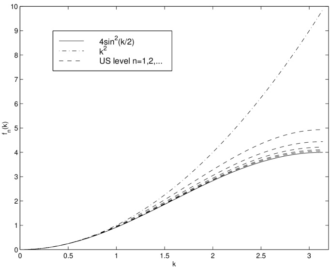
FIG. 1.: RG flow of the dynamics operator. In this case the starting point is a microscopic Laplacian operator of the form $L_{0,\omega}=i\omega+\frac{1}{\epsilon^{2}}k^{2}$. The functional form of the $n^{\rm th}$ iterate of $L_{\omega}$ is, $(L_{\omega,n})^{-1}=\frac{1}{2^{n}}\frac{\alpha_{n}}{i\omega\beta_{n}+\frac{1}{\Delta x_{n}^{2}}f_{n}(k)}$.

For the iterative process starting from, for instance, the microscopic action operator $H_{0}=\omega^{2}+\left[\frac{4}{\epsilon^{2}}\sin^{2}\left(\frac{k}{2}\right)\right]^{2}$, we take

$$H_{n}^{-1}=\frac{a_{n}+e_{n}\sin^{2}(\frac{k}{2})}{b_{n}^{2}\omega^{2}+(d_{n}\omega+\frac{4}{\Delta x_{n}^{2}}\sin^{2}(\frac{k}{2}))^{2}}\,,$$ (30)

where $d_{n}$ and $b_{n}$ are the real and imaginary parts of $\beta$ in $L_{n,\omega}$. The iteration relations for $a_{n}$ and $e_{n}$ are

$$a_{n+1} = a_{n}+2a_{n}d_{n}\frac{\Theta_{n}}{4}+(2a_{n}+e_{n})(b^{2}_{n}+d^{2}_{n})\left(\frac{\Theta_{n}}{4}\right)^{2}\,,$$ (31)

$$e_{n+1} = \frac{1}{4}\left(e_{n}+4e_{n}d_{n}\frac{\Theta_{n}}{4}-2a_{n}\right)\,.$$ (32)

The fixed point solutions are, setting $\theta_{n}=\sqrt{\Theta_{n}/2}$,

$$\begin{array}[]{rclclcl}a_{n}&=&1+\frac{\Theta_{n}^{2}}{360}+\cdots&=&\sum\frac{\Theta_{n}^{2i}}{(4i+3)!}[4^{i+1}]-\frac{1}{2}e_{n}&=&\frac{1}{4\theta_{n}^{3}}(\sinh(2\theta_{n})-\sin(2\theta_{n}))-\frac{1}{2}e_{n}\\ e_{n}&=&-\frac{2}{3}+\frac{4\,\Theta_{n}^{2}}{7!}+\cdots&=&\sum\frac{\Theta_{n}^{2i}}{(4i+3)!}[4(-1)^{i+1}]&=&\frac{1}{\theta_{n}^{3}}(\sinh(\theta_{n})\cos(\theta_{n})-\cosh(\theta_{n})\sin(\theta_{n}))\\ b_{n}&=&1-\frac{\Theta_{n}^{2}}{360}+\cdots&=&\sum\frac{\Theta_{n}^{2i}}{(4i+2)!}[2(-1)^{i}]&=&\frac{1}{\theta^{2}}\sinh(\theta_{n})\sin(\theta_{n})\\ d_{n}&=&-\frac{\Theta_{n}}{6}+\cdots&=&\sum\frac{\Theta_{n}^{2i+1}}{(4i+4)!}[2(-1)^{i+1}]&=&\frac{1}{\theta^{2}}(\cosh(\theta_{n})\cos(\theta_{n})-1)\,.\end{array}$$ (37)

We can now move on to the CG case. Here we parameterize the operators as

$$L_{\omega,n}^{-1} = \gamma_{n}\,\frac{\Delta x_{n}^{2}}{4}+\frac{\alpha_{n}}{i\omega\beta_{n}+\frac{4}{\Delta x_{n}^{2}}\sin^{2}(\frac{k}{2})}\,,$$ (38)

$$H_{n}^{-1} = f_{n}\,(\frac{\Delta x_{n}^{2}}{4})^{2}+\frac{a_{n}+e_{n}\sin^{2}(\frac{k}{2})}{b_{n}^{2}\omega^{2}+(d_{n}\omega+\frac{4}{\Delta x_{n}^{2}}\sin^{2}(\frac{k}{2}))^{2}}\,.$$ (39)

It is easy to see that CG shares the same $\beta$, $b$ and $d$ parameters with US. The iteration relations for the other parameters are different. However, one can obtain a relation between $\alpha^{CG}$ and $\alpha^{US}$, namely,

$$\alpha^{CG}_{n}=\alpha^{US}_{n}\beta_{n}=\frac{1}{i\Theta_{n}}\left(\alpha^{US}_{n+1}-\alpha^{US}_{n}\right)\,.$$ (40)

Using this relation we find

$$\gamma^{CG}_{n}=\frac{4}{i\Theta_{n}}(1-\alpha_{n}^{US})\,.$$ (41)

Therefore, the fixed point solution for $\alpha^{CG}$ and $\gamma^{CG}$ can be written in terms of that of $\alpha^{US}$, while the rest of the parameters have fixed points

$$\begin{array}[]{llll}a_{n}&=1-\frac{\Theta_{n}^{2}}{144}+\cdots&=\sum\frac{\Theta_{n}^{i}}{(4i+5)!}[2^{2i+4}(RI-1)]-\frac{1}{2}e_{n}&=(\cosh(\theta_{n})-\cos(\theta_{n}))^{2}Z_{n}\\ e_{n}&=-1+\frac{85\,\Theta_{n}^{2}}{3\cdot 7!}+\cdots&=\sum\frac{(-\Theta_{n})^{i}}{(4i+5)!}[8-2^{4i+7}]&=\frac{2}{\theta_{n}^{4}}(Z_{n+1}-Z_{n})\\ f_{n}&=\frac{2}{15}-\frac{16\,\Theta_{n}^{2}}{9!}+\cdots&=\sum\frac{\Theta_{n}^{i}}{(4i+5)!}[16(-1)^{i}]&=-\frac{4}{\theta_{n}^{4}}(Z_{n}-1)\,,\end{array}$$ (45)

where $Z_{n}\equiv\frac{1}{2\theta_{n}}[\cosh(\theta_{n})\sin(\theta_{n})+\sinh(\theta_{n})\cos(\theta_{n})]$, and $RI$ denote the average of real and complex parts of $(\frac{3+i}{2})^{4n+5}$.

B Perfect Action Operator in Space-Time and Stochastic CG Scheme

So far, we have only coarse grained the spatial degree of freedom and obtained the corresponding perfect operators. In order to move on to numerical calculations on a lattice, we also need to coarse grain the time degree of freedom.

We focus on the perfect action operator $H=\hat{L}^{T}_{\omega}\,\rho\,\hat{L}_{\omega}$ which is used later in the space-time Monte Carlo calculations. Here we derive the fixed point solution of $H$. We give a nearly closed form solution for $H(k,\omega)$ and show that this operator gives a perfect dispersion relation as measured from the time displaced two point function. The stochastic coarse graining scheme is introduced, which modifies $H$ to give us an operator with reduced range of interaction.

The iterative relation we developed previously does not hinge on whether CG was carried out on the space or time axis. Therefore, we can use it to CG in the time direction as well. Either one can start from a continuous description and alternately CG in space and in time, or one can directly use the perfect operator we developed previously and only CG from continuous time. Now, there is another dimensionless parameter, namely the ratio of the time scale over the characteristic time appropriate for a chosen length scale. For the diffusion equation, it is $\Delta t/\Delta x^{2}$. We already see the manifestation of this parameter in the perfect operator derived earlier, where only the combination of the form $\omega\Delta x^{2}$ enters the expressions. Therefore, there are two restrictions on how we apply the two schemes. In the first case, we should CG twice in time direction for each CG operation in the spatial direction, maintaining the value of the ratio $\Delta t/\Delta x^{2}$ throughout the process. This means, for any reasonable values of $\Delta t/\Delta x^{2}$ at the macroscopic side, we need to start with a small $\Delta x$ and a very small $\Delta t$. In the second case, we will not be able to maintain the ratio of $\Delta t/\Delta x^{2}$. Therefore, the fixed point operator should be identified by iterating backwards. This means, we repeat the iterative process many times starting from various values of $\Delta t_{n}\equiv\Delta t/2^{n}$ and iterate $n$ steps. The fixed point is identified as the operator which is (within tolerance) not changed whether we start from $\Delta t_{n}$ or $\Delta t_{n+1}$. This method was used in the previous section to calculate the fixed point operator form for $H$ when the time frequency $\omega$ was nonzero. This reversed iteration scheme is more powerful, since it can be generalized to other cases where there are other dimensionless parameters, such as in the case of massive fields.

The fixed point solution of a $d$-dimensional operator under the CG iterative relation can be found using the techniques that have been described in this paper. An alternative method, the so-called “blocking from continuum” can also be used. In either case one finds[20, 21, 22],

$$O_{\mathrm{FP}}({\bf k})^{-1}=\sum_{\bf l}O(({\bf k}+2\pi{\bf l})/{\bf\Delta x})^{-1}\,\prod_{d=1}^{D}\frac{4\sin^{2}(k_{d}/2)}{(k_{d}+2\pi l_{d})^{2}}+\frac{1}{\kappa_{0}}\,,$$ (46)

where $O({\bf p})$ is the continuum spectrum of the operator and ${\bf l}$ is a vector whose elements are of all possible integer values.

In the above equation, an extra constant term with a parameter $\kappa_{0}$ is introduced. This term is important for obtaining a localized perfect operator fit for numerical simulations[22]. To get this term, we modify the CG procedure to be a stochastic CG operation, also called soft CG, instead of hard CG, where an artificial noise term is introduced into the CG variable,

$$\phi^{S}=\bar{\phi}+\nu\,,$$ (47)

where $<\nu>=0$ and $\langle\nu({\bf i})\,\nu({\bf i}^{\prime})\rangle=\frac{\Omega}{\kappa_{0}\Delta V}\delta_{{\bf i},{\bf i}^{\prime}}$. Taking $\kappa_{0}\rightarrow\infty$, the hard CG case is recovered.

Now consider the diffusion equation for a massive field,

$$\partial_{t}\phi=\partial_{x}^{2}\phi-m\,\phi+\eta\,.$$ (48)

The continuum spectrum of $H$ is,

$$H=(\frac{\omega}{\Delta t})^{2}+[(\frac{k}{\Delta x})^{2}+m]^{2}\mbox{\ \ \ where \ \ }\omega,k\in(-\pi,\pi)\,.$$ (49)

Defining the notation $x_{l}=x+2\pi l$, we have,

$$\frac{1}{\Delta x^{4}}\,H^{-1}=\,\sum_{l,l^{\prime}}\frac{1}{(k_{l}^{2}+\mu)^{2}+r^{2}\,\omega_{l^{\prime}}^{2}}\frac{4\sin^{2}(k/2)}{k_{l}^{2}}\frac{4\sin^{2}(\omega/2)}{\omega_{l^{\prime}}^{2}}+\frac{1}{3\,r^{2}\,\kappa}\,,$$ (50)

where we defined parameters $\mu\equiv m\Delta x^{2}$ and $r\equiv\Delta x^{2}/\Delta t$. To conform with notations used in quantum field theories, we have defined $\kappa=\kappa_{0}\,\Delta t^{2}/3$.

The double summation is cumbersome to evaluate numerically due to its power decaying behavior. By rewriting the factor $\{k^{2}_{l}[(k^{2}_{l}+\mu)^{2}+r^{2}\omega^{2}_{l^{\prime}})]\}^{-1}$ as a difference of two terms we can re-express the above formula as a sum of a closed formed expression and an exponentially decaying expression. To do so, it is convenient to introduce $\omega^{*}_{l}\equiv(k_{l}^{2}+\mu)/r$ and the function

$$G(k,\mu)\equiv\sum_{l}\frac{4\sin^{2}(k/2)}{k_{l}^{2}(k_{l}^{2}+\mu)}=\frac{1}{\mu}\{1-\frac{(\sinh\sqrt{\mu})(1-\cos k)}{\sqrt{\mu}((\cosh\sqrt{\mu})-\cos k)}\}\}\,.$$

Then, after some simple algebraic manipulation, one finds

$$\frac{1}{\Delta x^{4}}\,H^{-1}=-\partial_{\mu}G-r\,\sin^{2}(\frac{\omega}{2})\,\partial^{2}_{\mu}G+2r\,\sin^{2}(\frac{\omega}{2})\sum_{l}\frac{4\sin^{2}(k/2)}{k_{l}^{2}(k_{l}^{2}+\mu)^{3}}\frac{e^{-\omega^{*}_{l}}-\cos\omega}{\cosh\omega^{*}_{l}-\cos\omega}+\frac{1}{3\,r^{2}\,\kappa}\,.$$ (51)

Now what remains of the summation is much easier to evaluate due to its exponential decaying behavior.

From the above equation, we can obtain the dispersion relation implied by such an operator. The two point function for a free field is $S(k,\omega)=H^{-1}(k,\omega)$. Taking the discrete Fourier transform of equation (51) back to real time gives the static equal time structure factor,

$$S(k,t=0)=\sum_{l}\frac{4\sin^{2}(k/2)}{k_{l}^{2}}\frac{1}{(\omega^{*}_{l})^{3}}(\omega^{*}_{l}-1+e^{-\omega^{*}_{l}})+\frac{1}{3r^{2}\,\kappa}\,,$$ (52)

and the time displaced two point function

$$S(k,t\geq 1) = \sum_{l}\left\{\frac{4\sin^{2}(k/2)}{k_{l}^{2}}\frac{4\sinh^{2}(\omega^{*}_{l}/2)}{(\omega^{*}_{l})^{2}}\right\}\frac{1}{2\omega^{*}_{l}}e^{-\omega^{*}_{l}t}$$ (53)

$$= \sum_{l}\frac{4\sin^{2}(k/2)}{k_{l}^{2}}\frac{1-2e^{-\omega^{*}_{l}}+e^{-2\omega^{*}_{l}}}{2(\omega^{*}_{l})^{3}}e^{-\omega^{*}_{l}(t-1)}\,.$$ (54)

All dynamic modes are present, each with the correct decaying behavior and with a prefactor (enclosed in curly bracket) due to coarse graining in space as well as in the time direction. In principle, the decay rate should be measured in the long time limit where all modes outside the first Brillouin zone are negligible. However, for all practical purposes, the $l\neq 0$ modes are negligible (or more precisely, the next significant mode not degenerate with $l=0$) even for short times. For example, for $k=\pi/2$, $\mu=0$, the amplitude of the next most significant mode ($l=-1$) is only $1.5\times 10^{-4}$ of that of the $l=0$ mode. Therefore, we can use the $t\geq 1$ values of the time displaced two point function to evaluate the perfect dispersion relation for all the wave modes with wavenumber within the first Brillouin zone.

From $H^{-1}(k,\omega)$, we obtain the perfect operator coefficients $H(r,t)$ in real space and time. Notice that “the fixed point of an operator” actually means the fixed point of the dimensionless operator. Consequently, operator coefficients for the perfect action operator are actually those of $H\,\Delta x^{4}$. For practical reasons, we need to adjust the parameter $\kappa$ for optimal locality. In one dimension, $\kappa\approx 2$ and 6 are the best values for $\partial_{x}^{2}$ and $\partial_{x}^{4}$ respectively. Therefore, we need to find a compromise. The best scheme is to choose $\kappa=2$ such that the most significant couplings lie within a rectangle area elongated along the $x$ direction. This way, the total number of significant couplings is minimized.

The leading order coefficients of $H$ for $\kappa=2$ and zero mass are tabulated in Table I and are shown in Figure 2.

TABLE I.: Sample coefficients of the perfect action operator for the diffusion equation. $\kappa=2$, $\mu=0$ and $\Delta x^{2}/\Delta t=1$.

$(t,x)$	$H$	$(t,x)$	$H$	$(t,x)$	$H$	$(t,x)$	$H$
(0, 0)	3.90458	(0, 1)	-1.02978	(0, 2)	-0.0421266	(0, 3)	0.098042
(0, 4)	0.0291451	(0, 5)	-0.00317113	(0, 6)	-0.00407848	(0, 7)	$-7.35334\times 10^{-4}$
(1, 0)	-0.464966	(1, 1)	-0.278677	(1, 2)	-0.0339122	(1, 3)	0.0328692
(1, 4)	0.0148371	(1, 5)	$-2.8286\times 10^{-4}$	(1, 6)	-0.00204057	(1, 7)	$-5.22915\times 10^{-4}$
(2, 0)	$-5.99324\times 10^{-4}$	(2, 1)	$-8.25418\times 10^{-4}$	(2, 2)	$-3.68371\times 10^{-4}$	(2, 3)	$6.91673\times 10^{-4}$
(2, 4)	$8.04927\times 10^{-4}$	(2, 5)	$2.04135\times 10^{-4}$	(2, 6)	$-1.27393\times 10^{-4}$	(2, 7)	$-9.25806\times 10^{-5}$

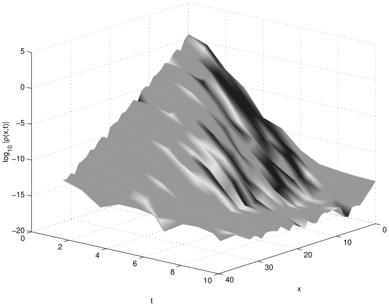
FIG. 2.: Surface plot of amplitude of perfect action operator coefficients for the diffusion equation. The coefficients exponentially decay away from the origin. The decay speed is slow along the $x$ direction. $\kappa=2$, $m=0$ and $\Delta t=\Delta x^{2}$.

IV Numerical Simulation Using the Perfect Operator

In this section, we discuss the application of the perfect linear operator in numerical simulations of Langevin dynamics. We show that the perfect operator should be decomposed into an Up operator and a Down operator in order to obtain a correct equation with a finite number of high order time derivatives. Without this decomposition, the truncation of the perfect operator is highly non-trivial, if not impossible. For Langevin dynamics, the dynamics of the non-Markovian noise is difficult to obtain because it requires taking the square root of the noise correlation function. Various numerical simulations were carried out using the truncated perfect operator and other approximations, to illustrate the advantage of using coarse grained variables as opposed to uniformly sampled variables in numerical simulations. These, together with the limitations of this approach, are also discussed.

A Perfect Operators in Langevin Dynamics

Here we derive the perfect operators $\hat{U}$ and $\varrho$ appropriate for Langevin dynamics. In the previous section, we obtained the iterative relation for both $\hat{L_{\omega}}$ and $H$. From the latter, the correlation function for the non-Markovian noise is obtained. The discretized system follows the dynamics described by the PDE,

$$\hat{L_{\omega}}\phi=\eta\,,$$ (55)

where $\eta$ satisfies $\langle\eta(i,j)\,\eta(i^{\prime},j^{\prime})\rangle=\frac{\Omega}{\Delta V}\rho^{-1}(i-i^{\prime},j-j^{\prime})$. This formally simple equation is different from the usual Langevin dynamics in two respects: the non-Markovian nature of noise and the presence of (in principle) infinite orders of time derivatives in both $\hat{L_{\omega}}$ and $\rho^{-1}$.

The non-Markovian nature of the noise means that there is dynamics in the noise variable. This is not surprising. In the path-integral calculation, each CG step results in formally discarding small scale degrees of freedom. But in fact, the small scale degrees of freedom are not entirely discarded. Since the small scale dynamics is affected by the noise source as well as the system dynamics at the coarse grained level, when the small scale degrees of freedom are integrated out at each CG step, part of the small scale dynamics is preserved by modifying the dynamics at the larger length scale and by injecting dynamics into the noise. This is basically a feedback effect.

Due to the non-Markovian nature of the noise, we need to write down the dynamics followed by the noise,

$$\rho^{1/2}\eta=\eta_{0}\,,$$ (56)

where $\eta_{0}$ is a white noise satisfying $\langle\eta_{0}(i,j)\,\eta_{0}(i^{\prime},j^{\prime})\rangle=\frac{\Omega}{\Delta V}\delta_{i,i^{\prime}}\,\delta_{j,j^{\prime}}$. The matrix $\rho^{1/2}$ is the square root of $\rho$ in the sense that the product of $\rho^{1/2}$ and its Hermitian conjugate gives $\rho$. For instance, in Fourier space, $\sqrt{\omega^{2}+k^{4}}=i\omega+k^{2}$. There are in principle infinite orders of time derivatives in $\rho^{1/2}$, just as in $\hat{L_{\omega}}$.

Naively, $\hat{L_{\omega}}$ can be obtained as a series expansion in $\partial_{t}$ which is then truncated to certain order. This turns out not to be the correct approach. Rather, we need to decompose the operator $\hat{L_{\omega}}$ in the form of a numerator ($\hat{U}$) over a denominator ($\hat{D}$),

$$\hat{L_{\omega}}\equiv\hat{D}^{-1}\hat{U}\,,$$ (57)

where we write the denominator as an inverse operator. The distinction between the numerator and denominator is easily seen in the fixed point operator. We can eliminate the inverse operator by applying $\hat{D}$ on both sides of equation (55). Redefining the noise as $\xi=\hat{D}\eta$ and denoting its correlation function $\varrho^{-1}$, we have,

$$\hat{U}^{-1}\varrho^{-1}\hat{U}^{T}\,{}^{-1}=\hat{L}^{-1}\rho^{-1}\hat{L}^{T}\,{}^{-1}\,.$$ (58)

The operators $\hat{U}$ and $\varrho$ are therefore equivalent to the older pair of $\hat{L}$ and $\rho$ in the evolution of the discretized system. Equation (55) may be rewritten as

$$\hat{U}_{\omega}\phi=\xi\mbox{\ \ \ \ with \ \ \ \ }\varrho^{1/2}\xi=\eta_{0}\,.$$ (59)

Using (39), and in the notation of the last section, the perfect operators for the diffusion equation under the CG scheme are

$$\hat{U}_{\omega} = i\omega\beta+\frac{4}{\Delta x^{2}}\sin^{2}\frac{k}{2}\,,$$ (60)

$$\varrho^{1/2} = \{\alpha+\gamma\,\sin^{2}\frac{k}{2}+\gamma\,\beta\frac{i\Theta}{4}\}/\{a+e\,\sin^{2}\frac{k}{2}+f\,b^{2}\,(\frac{\Theta}{4})^{2}+f\,(d\,\frac{\Theta}{4}+\sin^{2}\frac{k}{2})^{2}\}^{\frac{1}{2}}\,.$$ (61)

For analytical tractability, we used the closed-form solutions of the operators available for discrete space but continuous time.

Unlike $\hat{L}$, the new evolution operator $\hat{U}$ can be expressed in a clear and simple series expansion. The spatial part is simply the central difference operator and the time part is a sum of all orders of time derivatives with constant and fast decaying coefficients (see equation (29)).

The operator $\varrho^{1/2}$ has a very complicated form. It has many high order space and time derivatives, which in general are coupled. Series expansion and truncation are necessary. To the first order in $\Delta x^{2}$, we have for CG,

$$\varrho^{1/2}\approx 1-\frac{1}{6}\,\sin^{2}(k/2)+c\,i\omega\,\Delta x^{2}=1+\lambda^{2}\,\partial_{x}^{2}-\tau\partial_{t}\,,$$ (62)

where $c=1/6-1/\sqrt{720}=0.129$, $\lambda\equiv\Delta x/\sqrt{24}$ and $\tau\equiv c\,\Delta x^{2}$. Therefore, the noise source is largely a white noise. It has a correlation length of the order $\lambda$ and a relaxation time of the order $\tau$. When the form of the operator is obtained and truncated to a specified order, one can evolve the system according to equation (59).

Often periodic boundaries are used in the spatial dimensions. Therefore high order spatial derivatives do not pose a problem on a lattice. Higher order time derivatives, however, require a corresponding number of initial conditions. This might pose a problem, especially for the non-Markovian noise. If one is interested in equilibrium properties of the system, the initial transient stage is not important. An initial condition with all derivatives zero is fine. When one wants to study the initial transient stage corresponding to a certain microscopic initial condition, one can evolve the system using a fine mesh for $n$ steps under a conventional numerical scheme, where $n$ is the highest order time derivatives. For each step, one can coarse grain the microscopic configuration to the desired CG level, insert the CG version of $\phi$ into equation (59), and the noise in the transient stage is obtained. This way, initial time derivatives for both coarse grained $\phi$ and $\xi$ can be computed.

The calculation of the space-time discretized $\varrho^{1/2}$ can be quite involved[23]. Since our main interest is in calculating equilibrium properties of dynamic systems, we can take an alternative route, namely Monte Carlo simulation, as discussed later. In this case, the perfect action operator $H$ is all we need.

B An Example of Using Perfect Operator in Langevin Dynamics

In this section, we present an application of the operator $\hat{U}$ to the deterministic dynamics of the coarse grained variable governed by the diffusion equation. The (truncated) perfect operator $\hat{U}$ gives superior results for the evolution of the configuration. The relative advantage of using the CG variable vs the US variable is also touched upon and will be studied more closely in the ensuing section.

For simplicity, we truncate the series expansion of $\beta$ to the first order to obtain an operator $\hat{U}$ with a second order time derivative. Direct truncation is not appropriate when setting higher order terms to zero, since we should adjust the remaining coefficients. Instead, we use the operator at the first level of CG, starting from a central difference operator. The coefficients for time derivatives higher than the second order are identically zero. We have,

$$\frac{\Delta x^{2}}{16}\partial^{2}_{t}\phi_{i}+\partial_{t}\phi_{i}+\frac{1}{\Delta x^{2}}(2\,\phi_{i}-\phi_{i+1}-\phi_{i-1})=0.$$ (63)

Suppose the system is periodic with length $L$. The initial condition has modes down to length scale $\epsilon=L/M$ with $M$ being an integer, namely,

$$\phi(m,t=0)=\sum^{M/2}_{k=-M/2}e^{i2\pi k\,m\epsilon/L}\phi_{k}\,,$$ (64)

where $\phi_{k}$ is the amplitude of the $k$th wave mode. We know analytically the exact solution: by coarse graining the exact solution to a length scale $\Delta x=L/N=p\,\epsilon$, we have,

$$\bar{\phi}(n,t)=\sum^{N/2}_{q=-N/2}e^{i\frac{2\pi q\,n\Delta x}{L}}\sum^{p/2}_{i=-p/2}\phi_{q+i\,N}\frac{\sin(\pi q\Delta x/L)}{p\sin(\pi(q+i\,N)\epsilon/L)}e^{-(\frac{2\pi q\Delta x}{L})^{2}t}\equiv\sum^{N/2}_{q=-N/2}e^{i\frac{2\pi q\,n\Delta x}{L}}\bar{\phi}_{q,0}(t)\,,$$ (65)

where $\bar{\phi}_{q,0}(t)$ is the exact wave mode for the CG variable. This equation gives us both $\bar{\phi}(n,t=0)$ and $\partial_{t}\bar{\phi}(n,t=0)$. Now let us ask: what result would equation (63) yield on a lattice with grid size $\Delta x$, given the CG initial conditions? We have $\bar{\phi}_{q}(t)=\sum^{p/2}_{i=-p/2}C_{q,i}(t)\,\phi_{q+i\,N}$, where

$$C_{q,i}(t)=\frac{\sin(\pi q\Delta x/L)}{p\sin(\pi(q+i\,N)\epsilon/L)}e^{-\omega_{-}t}\,\{1+\frac{1-e^{-\Delta\omega\,t}}{\Delta\omega}[\omega_{-}-\frac{2\pi(q+i\,N)}{L^{2}}]\},$$ (66)

$\omega_{-}=\frac{16}{\Delta x^{2}}\sin^{2}(\frac{\pi q}{2N})$, and $\Delta\omega=\frac{16}{\Delta x^{2}}\cos(\frac{\pi q}{N})$. For comparison, the corresponding result from conventional numerical analysis (NA), which is the same as just keeping the first-order time derivative in $\hat{U}$, is

$$C^{NA}_{q,i}(t)=\exp\{-\frac{4\sin^{2}(\pi q/N)}{\Delta x^{2}}t\}\,,$$ (67)

where the time evolution does not depend on $i$. The solution for modes within the first Brillouin zone, i.e. $i=0$, is greatly improved as shown in Figure 3, where we have plotted the time evolution of the coefficient $C_{q,i=0}(t)$ (without the prefactor due to CG) for selected $q$ values. For small $q$, the $\Delta\omega$ dependent part in equation (66) is not important. A Taylor expansion clearly shows that $\omega_{-}$ is closer to the true decay rate than the NA result.

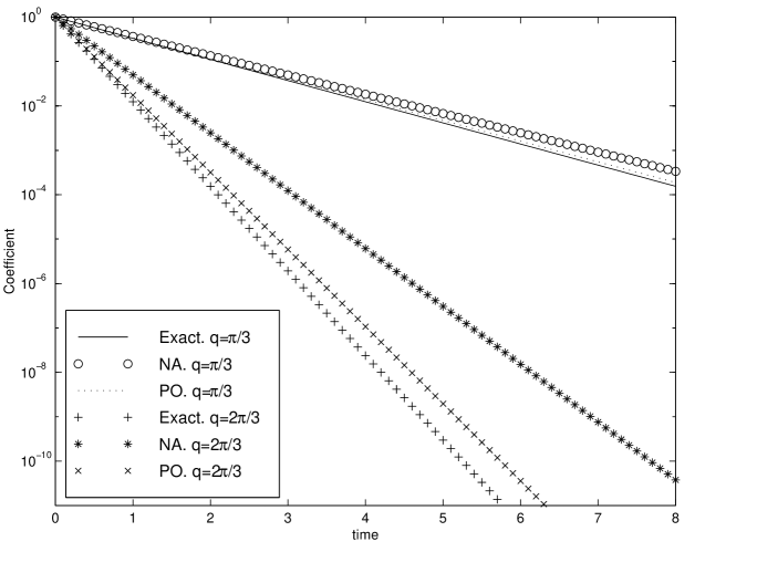
FIG. 3.: Decay of wave modes in the first Brillouin zone using PO and NA equations vs the exact result. The decay rates for the PO scheme are closer to the exact ones than the NA results. The coefficient is $C_{q,i=0}(t)$ without the CG prefactor. Sample wavenumbers are $q=\pi/3$ and $2\pi/3$.

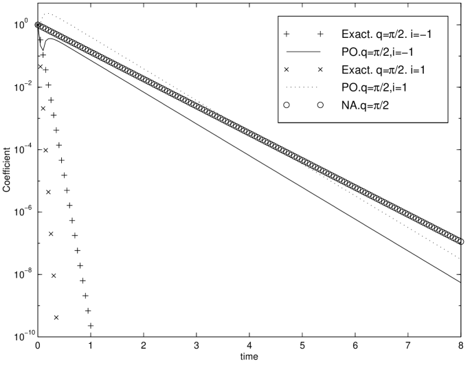
FIG. 4.: Decay of wave modes in the second $(i=-1)$ and third $(i=1)$ Brillouin zones using PO and NA equations vs the exact result. For the PO and NA schemes, wave modes do not decay as fast as for the exact result. PO is better for modes in the second Brillouin zone than NA and is also advantageous for late times for modes in other Brillouin zones. PO results are very close to the exact one at short times as indicated by the dip in the plotted curve. The coefficient is $C_{q,i=0}(t)$ without the CG prefactor, which reduces the importance of modes outside the first Brillouin zone. Sample wavenumber is $q=\pi/2$. Notice that the NA result does not depend on $i$.

For very short times, the dynamics of all modes are correctly prescribed, even for $i\neq 0$. This manifests itself as a dip in the short time region of Figure 4 (subject to resolution in the time axis, the dip for the $i=1$ mode is not discernible in the figure). For finite time, modes outside the first Brillouin zone decay quickly in the true dynamics (Figure 4). In the PO result, the decay rate is dependent on $q$, therefore these modes do not decay as fast as they should do. But since the PO result also contains information on $i$, for modes in the second Brillouin zone, the resulting dynamics are still closer to the true one than the NA result. This is because we used the PO operator $\hat{U}$ of one level CG. For higher wavenumbers, due to the $i$ dependent term, there is an anomalous (negative) amplification of wave modes at the initial transient stage which disappears later. Therefore, the power spectrum of the configuration should die off quickly for modes with length scale much less than $\Delta x$. In other words, we should not over-coarse-grain. It follows that as we keep more and more terms in the perturbative series for $\hat{U}_{\omega}$, the PO result will be close to the exact one for higher and higher wave modes.

The prefactor

$$\frac{\sin(\pi q\Delta x/L)}{\sin(\pi(q+i\,N)\epsilon/L)}$$

modifies the contribution of each wave mode to the solution. This comes from using the CG variable in the PDE and is very important in reducing errors that arise from using the discretized PDE. For instance, although modes with $q\approx 0$ decay very slowly in the PO result, their prefactor is close to zero for $i\neq 0$, while they very quickly decay to zero in the true dynamics.

Notice that US and CG share the same $\hat{U}$. In the US scheme, there is no prefactor. Modes with $q\approx 0$ and $i\neq 0$ do not decay. If we use the same equation as above, the prefactor for $t>\Delta x^{2}$ is,

$$C_{q\approx 0,i}(t)\approx 1-(\frac{i\pi}{2})^{2}\,.$$ (68)

For large $i$, it overstates the contribution of the mode to the solution and is worse than NA. This imposes a stricter constraint than for the CG scheme on the power spectrum of the configuration, and is the reason why CG is a better scheme. This has been tested numerically on several model dynamics[1].

V Space-Time Monte Carlo Simulation

The path-integral formulation easily leads to a space-time Monte Carlo simulation. We discuss issues related to truncating the perfect operator such that it has a finite range of interaction. Numerical simulations are carried out on the linear diffusion equation to test computational efficiency of using the perfect operator, and on Model A dynamics to test the merit of direct application of the perfect linear operator to nonlinear dynamics.

In quantum field theories, many problems are formulated in terms of path integrals. Numerical simulations usually employ the Monte Carlo method, where due to space-time symmetry, time is simply treated as one of the dimensions in a $d+1$-dimensional lattice. In statistical physics, when dynamics is involved, evolving a Langevin equation is the norm. A typical form of the equation contains a first-order time derivative, a diffusion term and some nonlinear interaction. Time and space are not symmetric. However, numerical simulation of a Langevin equation is not the only choice for studying dynamics. We can also perform Monte Carlo simulation on a space-time lattice[24], similar to the approach adopted in quantum field theories. The basis for such a calculation is the path-integral formulation. Starting from equation (3), and performing a trivial integration over the noise to eliminate the delta function, we have

$$P=\int D\phi\,\exp\{-\frac{\Delta V}{2\Omega}\sum_{i,j}[(\partial_{t}{\phi}+f(\phi))^{2}-\frac{\Omega}{\Delta x}\partial_{\phi}f]\}\,.$$ (69)

The cross term linear in $\partial_{t}$ results in a boundary term and does not influence directly the calculation of $P$. Ignoring the Jacobian contribution, we are left with a positive definite functional. We call the term in the exponent the ‘action’ for obvious reasons. For linear operators, we know how to coarse grain the above expression. Integrating out the noise in the above equation, we have

$$P=\int D\bar{\phi}\,\exp\{-\frac{\Delta V}{2\Omega}\sum\phi\,H\,\phi\}\,,$$ (70)

where $H$ is the fixed point operator of the action operator. Working with this path-integral formulation, we do not have to worry about taking the square root of the noise correlation matrix as we would with the Langevin equation.

In the following, we will look at a specific example of the linear theory, namely the dynamics of a system described by the diffusion equation,

$$\partial_{t}\,\phi=\partial_{x}^{2}\,\phi-m\,\phi+\eta\,,$$ (71)

where $m$ is a constant which we will call the mass and $\eta$ is white noise with strength $\Omega$. We have chosen a unit diffusion constant. In the space-time Monte Carlo probability we use the $1+1$-dimensional perfect operator for $-\partial_{t}^{2}+(-\partial_{x}^{2}+m)^{2}$ developed in the previous sections. Then we look at the application of the perfect linear operator to the nonlinear Model A dynamics.

A Truncated Perfect Operator

The perfect operator needs to be truncated to finite range to be used in numerical simulations. Although the introduction of stochastic CG reduced the interaction range of the perfect action operator, the operator coefficients do not terminate in a finite range. Furthermore, they decay slowly along the $x$ direction, where the coefficient of the 10th neighbor[25] still has an amplitude of around $1\times 10^{-5}$. This makes truncation of the perfect operator more problematic than in quantum field theories, where keeping next nearest neighbors is already very good[22].

One criterion for truncation is that the magnitude of the discarded coefficients have to be small. But there are other considerations as well[26, 27]. One would like the operator to satisfy certain constraints that stipulate the correct behavior of the operator in the continuum limit. These constraints are in the form of sum rules[22]. For the diffusion action above, the constraints in the continuous limit are,

$$\left\{\begin{array}[]{clcl}&\sum_{i}\sum_{j}H_{i,j}&=&\mu^{2}\\ \frac{1}{2}&\sum_{i}\sum_{j}H_{i,j}\,j^{2}&=&-r^{2}\\ \frac{1}{2}&\sum_{i}\sum_{j}H_{i,j}\,i^{2}&=&-2\mu\\ \frac{1}{4!}&\sum_{i}\sum_{j}H_{i,j}\,i^{4}&=&1\,,\end{array}\right.$$ (76)

where, as defined previously, $\mu=m\,\Delta x^{2}$ and $r=\Delta x^{2}/\Delta t$. Naively, one might expect that one way of proceeding would be to truncate the perfect operator to a finite and manageable range, and then to enforce these constraints to improve the directly truncated operator. In reality, these sum rules are not satisfied even for the perfect operator for finite $\Delta x$ and finite $\kappa$. The error is of higher order in $\Delta x$ and inversely proportional to $\kappa$. On the one hand, the continuous limit constraint conditions can be recovered. On the other hand, for finite $\Delta x$, the constraints no longer hold unless an operator with a long interaction range is used. The average constraint error is about $0.1\%$ if one keeps up to $\sim 20$ and $\sim 3$ neighbors in the $x$ and $t$ directions respectively.

TABLE II.: Coefficients of naturally truncated $11\times 3$ perfect action operator for diffusion equation. $\kappa=2$, $\mu\equiv m\Delta x^{2}=0.25$, $\Delta x^{2}/\Delta t=1$.

$(t,x)$	$H$	$(t,x)$	$H$	$(t,x)$	$H$	$(t,x)$	$H$
(0, 0)	4.00869	(0, 1)	-1.00198	(0, 2)	-0.0819891	(0, 3)	0.0724608
(0, 4)	0.0270167	(0, 5)	$3.546940\times 10^{-4}$	(0, 6)	-0.002564	(0, 7)	$-7.593954\times 10^{-4}$
(0, 8)	$4.298800\times 10^{-5}$	(0, 9)	$8.703907\times 10^{-5}$	(0, 10)	$1.817881\times 10^{-5}$	(1, 0)	-0.430984
(1, 1)	-0.265854	(1, 2)	-0.046095	(1, 3)	0.021651	(1, 4)	0.012848
(1, 5)	0.001211	(1, 6)	-0.001157	(1, 7)	$-4.724628\times 10^{-4}$	(1, 8)	$-6.542402\times 10^{-6}$
(1, 9)	$4.851149\times 10^{-5}$	(1, 10)	$1.406475\times 10^{-5}$	(2, 0)	$3.220461\times 10^{-4}$	(2, 1)	$-2.491026\times 10^{-4}$
(2, 2)	$-5.120127\times 10^{-4}$	(2, 3)	$1.844663\times 10^{-4}$	(2, 4)	$5.223556\times 10^{-4}$	(2, 5)	$2.386099\times 10^{-4}$
(2, 6)	$-2.442266\times 10^{-5}$	(2, 7)	$-5.894465\times 10^{-5}$	(2, 8)	$-1.676697\times 10^{-5}$	(2, 9)	$3.755505\times 10^{-6}$
(2, 10)	$4.507152\times 10^{-6}$

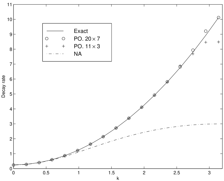
FIG. 5.: Decay rate of wave modes for diffusion equation. $\kappa=2$, $\mu=0.25$ and $\Delta x^{2}/\Delta t=1$. Perfect operator decay rates are obtained using the first two $t\neq 0$ nodes (equation (54)).

An alternative approach[26, 27] is to compute the perfect operator on a smaller lattice and then use this ‘naturally’ truncated perfect operator. In this way, the constraint is taken care of in the continuum limit. If we use the operator on a lattice of the same size, the operator gives a perfect dispersion relation. However, when it is used on a larger lattice, it is no longer perfect, as can be seen from the inexact dispersion relation for high wave number modes, which are those most affected by truncation. The reason lies in the high decay rate associated with a $k^{2}$ dispersion relation. For $k=\pi$, the ratio between successive $S(k,t)$ values is about $2\times 10^{4}$. Thus, to maintain exponentially decaying scaling over three nodes, we need a relative accuracy of $10^{-8}$. Taking into consideration the importance of keeping enough neighbors and the computational efficiency, an operator with up to 10th and 2nd neighbors in the $x$ and $t$ directions is chosen as the operator for most of the subsequent computer simulations. An operator with 9th and 2nd neighbors in the $x$ and $t$ directions is also used for some of the simulations. There is no discernible difference between this operator and the $11\times 3$ one.

The operator coefficients are displayed in Table II for $\mu=0.25$ and $\Delta t=\Delta x^{2}$. For the above operator with $\mu=0.25$, a 3 node scaling regime is maintained for 60$\%$ of the $k$ mode and a 2 node scaling regime for about 94$\%$ of $k$ mode. For a larger operator of size $20\times 7$, we would have a 3 node scaling regime for about 90$\%$ of the $k$ mode. The decay rates for different operators are compared in Figure 5.

The rapid decay rate of high wavenumber modes is what distinguishes the perfect operator for the diffusion equation from the $1+1$-dimensional Laplacian operator used in high energy physics. In the latter case, the ratio between successive $S(k,t)$ values is at the more benign level of about $0.04$. The exponential decaying range spans more values of time displacement. It is easier, therefore, to read off the dispersion relation all the way to the edge of the Brillouin zone. It is also more stable with respect to small changes in coefficients of the operator.

B Numerical Simulation of Diffusion Equation

We carried out space-time Monte Carlo simulations to test the efficacy of the perfect operator developed in the previous section. Suppose we are interested in the diffusion dynamics of the system described by equation (71) and would like to calculate its space-time correlation function. Let the system be of length $L=16$, with the spatial scale of interest $l=1$. In the path-integral formulation, the time span of the system is $T=8$. Both space and time directions have periodic boundary conditions. The Metropolis algorithm is employed[28].

Three simulation runs are presented. One simulation uses a perfect operator with range of interaction up to 10th and 2nd neighbor in the $x$ and $t$ directions respectively. A lattice of $N_{x}\times N_{t}=32\times 32$ was used, corresponding to $\Delta x=0.5$. The other two simulations were carried out on 32 $\times$ 32 and 64 $\times$ 128 lattices using the conventional central difference operator. In each case, the time direction grid size is $\Delta t=\Delta x^{2}$. In each simulation, $Nrun$ number of independent runs were conducted to obtain statistics of measurements, each run with $N=5\times 10^{5}$ MC steps (one sweep of the system) and one measurement per 8 steps. $Nrun=6$ and 7 for the 32 $\times$ 32 and 64 $\times$ 128 lattices respectively. The $(k\sim 0,\omega\sim 0)$ modes have the largest standard error, which is crucially dependent on the lattice size. The typical percentage standard error of $S(k,\omega)$ for 32 $\times$ 32 lattice is about $1\%$ and $2.5\%$ for PO and NA operators, while that of 64 $\times$ 128 lattice is $6\%$.

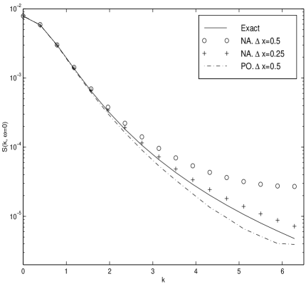
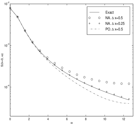
FIG. 6.: Cross sections of $S(k,\omega)$ for the diffusion equation. $m=1$, $L=16$, $T=8$. Cross sections are at $\omega=0$ (left) and $k=0$ (right). The exact result is $[(m+k^{2})^{2}+\omega^{2}]^{-1}$.

In Fourier space, cross sections of the space-time displaced two point function $S(k,\omega)$ are plotted in Figure 6. We do not expect the perfect operator result to be exact because $S(k,\omega)$ is now a two point function of the CGed variable, not the continuous variable. But it turns out to be quite close to the exact result. The NA result for 32 $\times$ 32 lattice deviates further from the true value at the same $(k,\omega)$ value. For this plot, a constant offset of $\frac{\Omega}{T\,L}\frac{\Delta x^{4}}{3\kappa}$ is subtracted from $S(k,\omega)$ of the perfect operator runs to eliminate the contribution from the added noise in the stochastic CG transformation.

Fourier transforming $S(k,\omega)$ to real time, we obtain the dispersion relation from $S(k,t)\sim e^{-\omega(k)t}$. To avoid static contributions in the $t=0$ mode, we choose the most significant $t\neq 0$ points to calculate $\omega(k)=(\log S(k,\Delta t)-\log S(k,2\Delta t))/\Delta t$. The results are shown in Figure 7. The perfect operator gives a near ‘perfect’ dispersion relation for the length scale we are interested in (corresponding to wavenumber $k\sim\pi$), giving the correct zero $k$ mode mass and correct $k^{2}$ dependence. We can get a comparable result using a larger lattice with the NA operator, but with more computational effort. For large $k$ modes, the amplitude of $S(k,2\Delta t)$ is of order $10^{-2}$ relative to that at $t=0$ and becomes unreliable given the simulation accuracy. The real value is used in the plot when $S(k,2\Delta t)$ is negative.

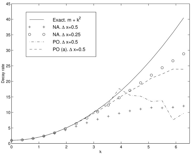
FIG. 7.: Decay rate of wave modes for the diffusion equation. $m=1$, $L=16$, $T=8$. Lattices yield $\Delta t=\Delta x^{2}$. Length scale of interest corresponds to $k\sim\pi$. Exact result is $m+k^{2}$. PO results use the first two $t\neq 0$ nodes of $S(k,t)$. NA results and PO (a) are obtained using the $t=0$ and $t=\Delta t$ nodes.

One might ask: why call the operator perfect when it does not reproduce the correct dispersion relation for wavenumbers beyond $k=\pi$? The answer is that it is not the operator that is not perfect but the simulation itself! The perfect operator gives the best result possible for physical quantities of interest given the error of the simulation. With more statistics, the dispersion relation from the perfect operator approaches the correct result for all modes with length scale larger than the grid size. The same is not true for the NA operator. For a discretization twice as fine, with increasing number of statistical samples, the dispersion relation for the NA operator approaches a limit that is different from the true solution, and is about $19\%$ off at the edge of the Brillouin zone.

The simulation error can be overcome when we choose smaller $\Delta t$ relative to $\Delta x^{2}$. As shown in Figure 8, the PO decay rates using $\Delta t=\frac{1}{2}\,\Delta x^{2}$ (corresponding to $32\times 64$ lattice) closely follows the exact result and is more accurate than the measurement from NA.

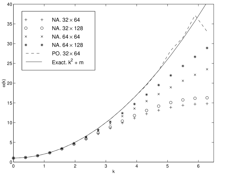
FIG. 8.: Decay rate of wave modes for the diffusion equation. $m=1$, $L=16$, $T=8$. Same as in Figure 7 except that lattices with $\Delta t\neq\Delta x^{2}$ are used.

One might as well choose operators according to the magnitude of the statistical error of a simulation. Given the usual error of $1\%$ for $S(k,\omega)$, a smaller sized perfect operator could be used to improve efficiency of the simulation without compromising accuracy of the physical measurements. Even with a $11\times 3$ PO as used in our simulation, the extra computational effort is not that huge. This operator requires $21\times 5=105$ points be used to calculate the action density at each grid point, whereas 7 points are used in conventional NA calculations. However, since most of the computation effort goes to generating random numbers (we used Numerical Recipe’s ran2() subroutine[29] as well as SPRNG modified lagged Fibonacci generator from NCSA[30]), it turns out that the overhead from extra neighbors is not significant considering the improvement of results. If one uses a naturally truncated $5\times 2$ PO, total CPU time for the sample calculation will be reduced by $58\%$. The decay rate rivals the result from NA with a lattice twice as large. In this case, however, we will not recover a perfect decay rate with better statistics due to the severe truncation.

Our code is written in C++. On a SUN Ultra2200, the run times are shown in Table III for a test run on a 32 $\times$ 32 lattice with 10000 MC steps. For the same number of steps and lattice size, the PO calculation takes about 4 times as much time as the NA calculation. Their standard errors for decay rates are roughly the same if the same nodes are used. However, the PO uses the second and third nodes to calculate decay rates. Therefore the resulting decay rates have standard errors about twice the size of that for NA.

TABLE III.: CPU time of simulations on diffusion equation using PO vs NA. 32 $\times$ 32 lattice. 10000 Monte Carlo steps. For the same number of statistical averages, the standard error of $S(k,\omega)$ for PO is about half of that for NA.

	Action Calculation	Random Number Generation	Total Time
NA	6.6s	15.0s	30.1s
PO	105.4s	13.6s	128.5s

The relevant quantity regarding the computational efficiency is the total computational effort (TCE) needed to reach a certain level of root mean square (RMS) error $\delta$. This is defined as

$$\mathrm{TCE}=c\,N\,N_{t}\,N_{x}\,,$$ (77)

where the speed factor, $c$, is 4 and 1 for PO and NA respectively. The RMS error $\delta$ is given by

$$\delta^{2}=\delta_{1}^{2}+\delta_{2}^{2}\,,$$ (78)

where $\delta_{1}$ is the bias and $\delta_{2}$ is the standard error. In comparing the efficiencies of PO and NA, we focus on the wave mode with $k=\pi$.

For the naturally truncated PO, $\delta_{1}\sim 0.01\%$ and is negligible. For a $32\times 64$ lattice, 64K MC steps are needed to reduce $\delta_{2}$ to $1\%$ for $k=\pi$. Hence $\mathrm{TCE}=5.2\times 10^{8}$.

For NA and a large lattice size, we have,

$$\delta_{1}\approx\frac{a}{N_{x}^{2}}+\frac{b}{N_{t}^{2}}\,,\ \ {\rm where}\ \ a=\frac{k^{4}\,L^{2}}{12\,(m+k^{2})}\ \ {\rm and}\ \ b=\frac{(m+k^{2})^{2}\,T^{2}}{24}\,.$$ (79)

For instance, with $L=16$, $T=8$, $m=1$, $k=\pi$, one has $a=191.2$ and $b=315.1$. The standard error $\delta_{2}$ is inversely proportional to $\sqrt{N}$ and is a function of the lattice size. Increasing the lattice size increases $\delta_{2}$. However, increasing $N_{t}$ also has the effect of improving the result, since smaller $\Delta t$ relaxes the constraint on the statistical accuracy of the first few nodes of $S(k,t)$. Let us assume that

$$\delta_{2}=\delta_{2}^{(0)}\,N_{x}^{\alpha}\,N_{t}^{\beta}/\sqrt{N}\,,$$ (80)

where $\alpha$ and $\beta$ are constant parameters. The minimization of the total computational effort yields,

$$N_{x}^{2} = (\frac{2+2\,\alpha+2\,\beta}{2\,\alpha+1})\,\frac{a}{\delta_{1}}\,,$$ (81)

$$N_{t}^{2} = (\frac{2+2\,\alpha+2\,\beta}{2\,\beta+1})\,\frac{b}{\delta_{1}}\,,$$ (82)

$$\frac{N}{N_{0}} = (1+\frac{1+\alpha+\beta}{2})\,(\frac{N_{x}}{N_{x,0}})^{2\alpha}\,(\frac{N_{t}}{N_{t,0}})^{2\beta}\,(\frac{\delta_{2}(N_{0},N_{x,0},N_{t,0})}{\delta})^{2}\,,$$ (83)

where the optimal $\delta_{1}=\delta/\sqrt{1+\frac{2}{1+\alpha+\beta}}$ and where $\delta_{2}(N_{0},N_{x,0},N_{t,0})$ is the $\delta_{2}$ value for a lattice size $(N_{x,0},N_{t,0})$ and with $N_{0}$ Monte Carlo steps. For instance, with the above $a$ and $b$ values and $\alpha=\beta=0$, to reach a RMS error of $1\%$, one needs $N_{x}=257$ and $N_{t}=330$. Given that $\delta_{2}\approx 1.2\%$ for $N_{0}=40K$, $N_{x,0}=128$ and $N_{t,0}=256$, we expect the optimal $N=86K$. Therefore $\mathrm{TCE}=7.3\times 10^{9}$. If we have $\alpha=1$ and $\beta=0$ instead, the optimal values are $N_{x}=190$ and $N_{t}=423$ and $N=254K$. Therefore $\mathrm{TCE}=2.0\times 10^{10}$. There is a factor of 40 improvement (see Table IV). The advantage of PO will be more pronounced in higher dimensions.

The values of $\alpha$ and $\beta$ are difficult to obtain. The values $\alpha=1$ and $\beta=0$ are good approximations for the relevant lattice sizes, namely $N_{x}$ and $N_{t}$ of order of or bigger than 200. Notice that a large lattice size is most detrimental to the standard error of the small $k$ modes.

TABLE IV.: Total computational effort for PO vs NA. One requires that the root mean error of $\omega(k)$ be $\delta=1\%$ for $k=\pi$. Parameters are $\alpha=1$ and $\beta=0$ (see equation (80)).

	$c$	$N_{x}$	$N_{t}$	$N$ ($\times 10^{3}$)	TCE ($\times 10^{8}$)
NA	1	190	423	254	200
PO	4	32	64	64	5.2

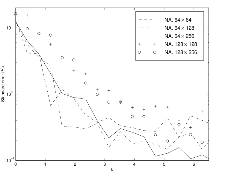
FIG. 9.: The standard error of the decay rate of wave modes for the diffusion equation for NA using different lattice sizes. $m=1$, $L=16$, $T=8$. Standard errors are normalized to $N=10^{5}$ Monte Carlo steps.

In summary, we find that the perfect linear operator gives us the perfect dynamics of the various wave modes, given the errors of a numerical simulation. For the same lattice size and number of Monte Carlo steps, the PO scheme (with the $11\times 3$ operator) is about 4 times slower relative to the NA scheme, where generating random numbers takes about $50\%$ of the total computation time in the latter case. However, the computational effort in order to reach the same root mean square error for PO is on the order of $1/40$ of that for NA. This will be more pronounced in higher dimensions. Moreover, a more severe truncation of the perfect operator is possible, given the inherent accuracy of the simulation, further enhancing the efficiency of the PO scheme.

C Numerical Simulations on Model A Dynamics

In this section we study the application of perfect linear operator to the time dependent Ginzburg-Landau equation for Model A dynamics,

$$\partial_{t}\,\phi=\partial_{x}^{2}\,\phi-m\,\phi-g\,\phi^{3}+\eta\,.$$ (84)

The corresponding path-integral formula is,

$$P=\int D\phi\,\exp\{-\frac{\Delta V}{2\Omega}\sum_{i,j}[S_{0}+S_{1}]\}\,,$$ (85)

where $S_{0}=\phi(-\partial_{t}^{2}+(-\partial_{x}^{2}+m)^{2})\phi$ and $S_{1}=2\,g\,\phi^{3}\,(-\partial_{x}^{2}+m)\phi+(g\,\phi^{3})^{2}-\frac{3g\,\Omega}{\Delta x}\phi^{2}$ are contributions from the linear and nonlinear terms respectively.

For systems with nonlinear interactions, an exact analytical expression for the perfect operator is not available. The difficulty lies in the fact that the form of the continuous action is not closed under the CG transformation. New interaction terms are generated in reaching the fixed point of the discrete description of the dynamics. In general there is an infinite number of interaction terms of diminishing importance. In order to proceed, we need to make some approximations. In conventional numerical analysis, the form of the continuous action is used, where the Laplacian operator is replaced by the central difference operator and local self-interactions are left unchanged. In analogy, we use the perfect linear operator developed previously for $S_{0}$, while leaving the nonlinear self interactions unchanged. We bundle the $m\phi$ term in with the $g\,\phi^{3}$ term in the $m<0$ regime to reduce the standard error of the numerical simulation. Intuitively this is a reasonable thing to do since $|\phi|$ develops a non-zero amplitude and the contribution to the dynamics of $\phi$ from these two terms largely cancel each other. We used the conventional central difference operator for the operator $-\partial_{x}^{2}+m$ in $S_{1}$.

There are two regimes: $m>0$ where the nonlinear term amounts to a renormalization of the mass, and $m<0$ where a nontrivial ground state develops with a magnitude $\pm\sqrt{m/g}$.

1 The $m>0$ Regime

We simulated the dynamics of a system of physical lengths $L=16$, $T=8$ and parameters $m=g=\Omega=1$ on lattices of different sizes. Mass dependent perfect linear operators are used. The Fourier transformed space-time correlation functions $S(k,\omega)$ are measured and averaged over several runs. Most simulations consist of $Nrun=9$ runs, each with $N=3\times 10^{5}$ Monte Carlo steps. Measurements are done every 8 Monte Carlo steps. For the NA result with $64\times 256$ lattice, 8 runs are used. Fourier transforming $S(k,\omega)$ to real time, we obtain $S(k,t)$, where $S(k,t=0)$ is the static structure factor and the mode decay rates can be read off from the time dependence of $S(k,t)$. The length scales of interest are those larger than $\Delta x=1$. As in the case of the diffusion equation, the standard error of the PO result is half of that for NA with the same number of statistical averages.

Mode decay rates obtained from the PO scheme for $k$ away from the origin are greatly improved over its NA counterparts, as shown in Figure 10. For $\Delta x=0.5$, $\Delta t=0.25$, if we had used the second and third nodes of $S(k,t)$, the decay rates for the second half of the Brillouin zone would not be reliable, reflecting the inherent numerical error (roughly $1\%$) of the simulation. This is as in the free field case discussed at the end of the previous section. For the plots, we used the $t=0$ and $t=\Delta t$ nodes instead. It is no longer perfect, but it is within the numerical error of the simulation and gives improved results as compared with NA. When we choose $\Delta t=0.125$, the error of the simulation is no longer a limiting factor and the decay rates over the whole Brillouin zone are recovered using PO. With a smaller $\Delta t/\Delta x^{2}$ ratio, the time direction becomes more continuous and the decay rate values are improved for all schemes as expected.

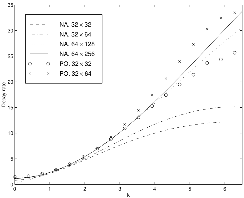
FIG. 10.: Decay rates of wave modes for the Ginzburg-Landau equation. $m=1$, $L=16$, $T=8$.

For $m>0$, the ground state of the order parameter has an expectation value of zero. The nonlinear self interaction term in equation (84) has the main effect of renormalizing the mass to a new effective mass $m_{\mathrm{eff}}=m+g\langle\phi^{2}\rangle$. In mean-field theory, the expectation value of $\phi^{2}$ is expressed as a function of $m_{\mathrm{eff}}$, which is then self-consistently determined by the relation

$$m_{\mathrm{eff}}/m=1+\frac{1}{m_{\mathrm{eff}}/m}\,(\frac{g\,\Omega}{4\,m^{3/2}})\,.$$ (86)

The renormalized mass is easily seen to be larger than the bare one.

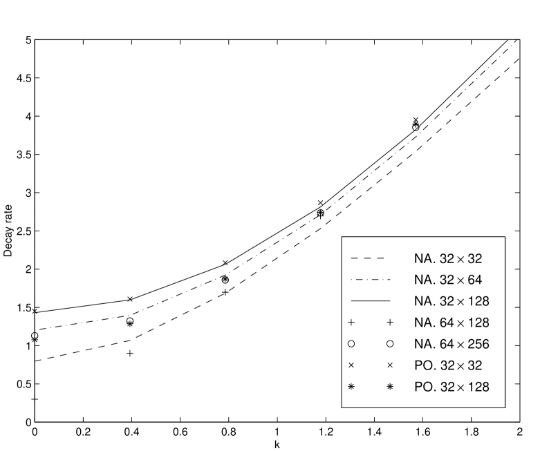
FIG. 11.: The influence of $\Delta t/\Delta x^{2}$ on the decay rate of small $k$ wave modes for the Ginzburg-Landau equation. Smaller $\Delta t$ gives improved result for NA. The effective mass for PO, however, approaches a limit less than the mean-field result. $m=1$, $L=16$, $T=8$.

From the decay rate of wave modes with $k\approx 0$, we can read off the value of the renormalized effective mass. The mean field value of the effective mass is $m_{\mathrm{eff}}=1.2258$ for the chosen parameters. For the NA scheme, the renormalized mass is less than the bare mass when the grid size along the time direction is chosen to be $\Delta t=\Delta x^{2}$. Reducing the grid sizes while retaining the ratio $\Delta t/\Delta x^{2}$ leads to reduced effective mass values, away from the correct result. For the $64\times 128$ lattice, we have $m_{\mathrm{eff}}\approx 0.26$. Unlike in quantum field theories, time and space are not symmetric in the dynamics we are considering. This translates into a freedom of choice of grid sizes $\Delta t$ and $\Delta x$. Physical considerations lead us to the natural choice of $\Delta t=c\cdot\Delta x^{z}$ where $z$ is the dynamic exponent and $c$ is a constant factor. Outside the critical regime, the diffusion term dominates the dynamics and $z$ equals the mean field value of 2. We expect the constant factor $c$ to be dependent on the nature of the nonlinear interaction and to be different from 1. When we over coarse grain in the time direction relative to the space direction, the (relatively) finite size of $\Delta t$ introduces error into the simulation results. We found that a $\Delta x^{2}/\Delta t$ ratio value of 2 to 4 is needed to reduce this error (see Figure 11).

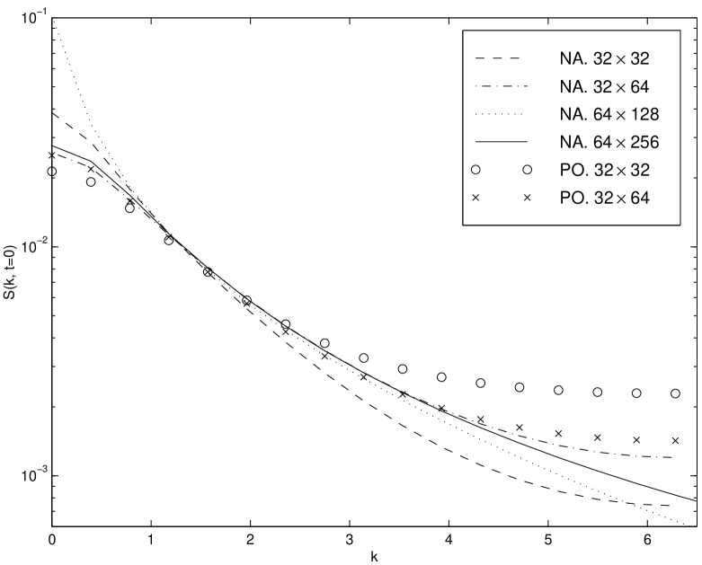
FIG. 12.: The static structure factor $S(k,t=0)$ for the Ginzburg-Landau equation. $m=1$, $L=16$, $T=8$.

For the PO scheme, the effective mass is above the bare mass for $\Delta t=\Delta x^{2}$. However, as $\Delta t$ is reduced, the effective mass decreases. For a $32\times 128$ lattice, the effective mass is found to be around 1.07. The reason lies in the fact that we used the simple central difference Laplacian operator in the nonlinear part of action $S_{1}$! We expect that the perfect linear operator operating on a function $f(x)$, which does not depend on $t$, should yield $(-\partial_{x}^{2}+m)^{2}\,f(x)$. However, a summation of the PO along the $t$ direction does not yield the one-dimensional NA form $(-\partial_{x}^{2}+m)^{2}$, but rather has coefficients roughly twice that of the NA form. Therefore, it is inconsistent to simply use the central difference form for operator $(-\partial_{x}^{2}+m)$. A test simulation using $\sqrt{2}\,(-\partial_{x}^{2}+m)_{\mathrm{NA}}$ gives the value 1.36 for the effective mass, closer to our expectation. However, it is not clear how to interpret this and it points to the need to derive the perfect form for the whole action including the nonlinear part.

For the static structure factor $S(k,t=0)$, shown in Figure 12, the PO result is not very close to the bench mark result of NA with a $64\times 256$ lattice. For large values of $k$, there is a contribution from the stochastic CG transformation. For small $k$ values, its deviation is a result of the inaccuracy in the effective mass, which is related to the correlation length $\xi$ (and hence the shape of $S(k)$) by the relation $\xi\sim m_{\mathrm{eff}}^{-1/2}$.

It is interesting to notice that the structure factor curves obtained using different schemes and lattice sizes all cross at the same point around $k\approx 1.3$.

2 The $m<0$ Regime

In this case, there is a non-trivial fixed point in the action which corresponds to a ground state with order parameter values $\phi=\pm\sqrt{m/g}$. Domains of opposite order parameter values compete and the dynamics is quite different from that with $m$ above 0. In our simulation, we used the same parameters as in the previous section except $m=-1$. We treat $m\phi+g\phi^{3}$ as one term and use the massless perfect linear operator. This leads to a reduced standard error. The data are plotted in Figures 13 and 14.

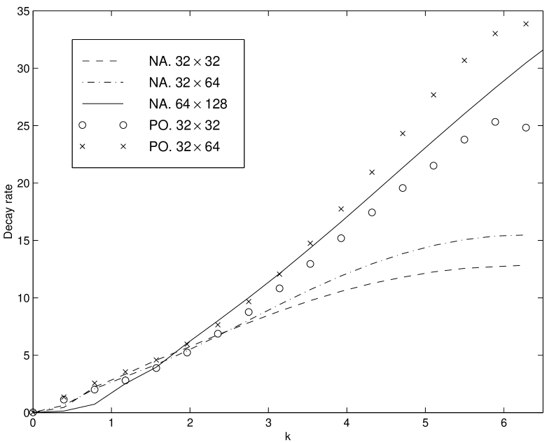
FIG. 13.: Decay rates of wave modes for the Ginzburg-Landau equation. $m=-1$, $L=16$, $T=8$.

The general shape and values of the dispersion relation are similar to those of the $m>0$ regime. However, there is a marked difference between these two regimes for wave modes close to $k=0$. Here, instead of approaching a finite effective mass, the decay rate approaches zero, reflecting the existence of a ground state with a non-zero amplitude. Also due to the ‘vanishing’ effective mass, the shape of the structure factor is more peaked at the origin than in the $m>0$ regime. For modes with small $k$ (first few nodes), $S(k,\omega)$ values have a large standard deviation. For example, it is about $25\%$ for the $k=4\pi/L$ mode and about $9\%$ for the $k=8\pi/L$ for NA on a $32\times 64$ lattice.

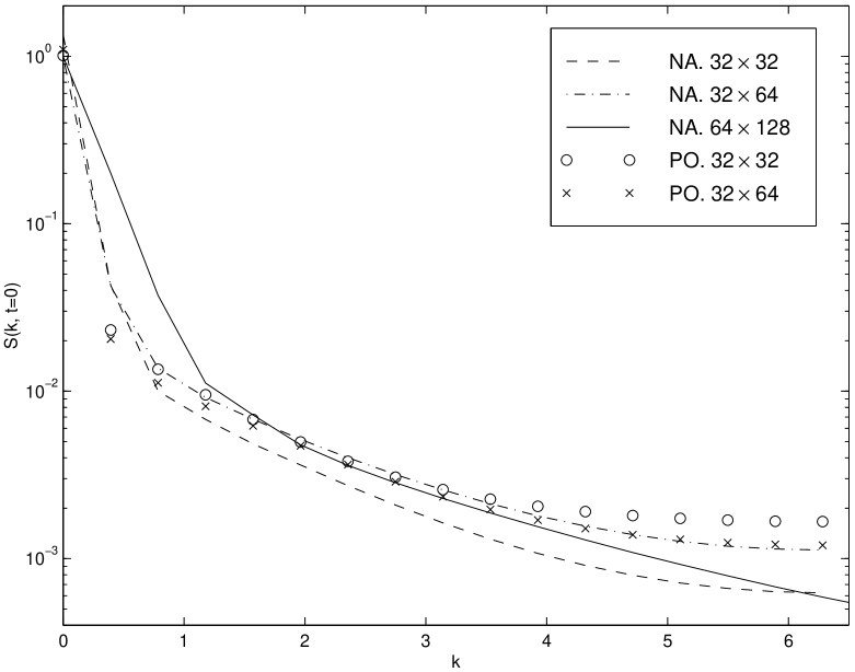
FIG. 14.: The static structure factor $S(k,t=0)$ for the Ginzburg-Landau equation. $m=-1$, $L=16$, $T=8$.

When grid sizes are reduced, the dispersion relation changes shape for small $k$ modes. The difference is significant with respect to the standard error. This has also been checked with increased statistics. This may be due to the existence of the non-trivial ground state. For $m<0$, there is another length scale in the problem, namely, the interface width between domains with opposite signs of the ground state order parameter value. If the grid size $\Delta x$ is not small enough, the position, and hence the dynamics, of the domain interface will not be resolved. This seems to be the reason why the shape of the dispersion relation for small $k$ values changes as $\Delta x$ is reduced, and it places an inherent physical constraint on the level of discretization one can reach. Only when this extra complication is taken into account can we obtain a perfect operator for this problem. Nevertheless, as shown in the figure, the perfect linear operator gives superior results to the NA operator for the same lattice size and computational effort (as discussed in the previous section).

In summary, a direct application of the perfect linear operator gives us an improved dispersion relation for Model A dynamics, especially for those modes with a length scale comparable to the lattice grid size. However, a more extensive study is needed to fully assess the efficacy of the perfect operator. This requires improving the perfect operator such that it yields the correct effective mass in the $m>0$ regime and accounts for the formation of domain interfaces in the $m<0$ regime.

D Modified ‘Perfect’ Operator

As previously shown, although the perfect operator coefficients fall off exponentially as one moves away from the origin, the decay rate is slow along the $x$ direction. Therefore, an operator with a shorter range of interaction is desired.

In non-linear $\sigma$ model[22], by simply including the next-nearest-neighbors (NNN), the dispersion relation can be greatly improved. In that case, the NNN coefficients are obtained using a natural truncation of the perfect operator. Since the operator coefficients fall off quickly along both $x$ and $t$ axis, such a severe truncation can still lead to significant improvement. This is no longer true for the diffusion equation. However, we might ask, can we improve the NA operator by allowing for non-zero operator coefficients for more neighbors? The answer is yes.

TABLE V.: Coefficients of the modified perfect action operator. $\mu=0$ and $\Delta x^{2}/\Delta t=1$.

$(x,t)$	$H$	$(x,t)$	$H$	$(x,t)$	$H$	$(x,t)$	$H$
(0, 0)	6.317206	(0, 1)	-3.050944	(0, 2)	$8.922786\times 10^{-1}$	(0, 3)	$6.200040\times 10^{-5}$
(1, 0)	$-4.396585\times 10^{-1}$	(1, 1)	$-2.637365\times 10^{-1}$	(1, 2)	$-3.045599\times 10^{-2}$	(1, 3)	$1.402178\times 10^{-2}$

We begin from the continuum limit constraints of equation (76). Setting $\mu=0$ and keeping $\rho(i,j)$ non-zero for $(i,j)\,\in\,\{(0,0),(0,1),(1,0),(2,0)\}$ (called the basic points), the conventional operator is obtained as the only solution to these equations. When more neighbors are included, the constraints are enforced by solving for $\rho$ of the basic points as function of the other coefficient values.

Using these non-basic-points coefficients as fitting parameters, we can obtain an operator with a near perfect dispersion relation. If two parameters ($H(1,1)$ and $H(2,1)$) are used to obtain a $3\times 2$ operator, the average error for the dispersion relation is about $6\%$. By fitting four parameters (by also including $H(3,0)$ and $H(3,1)$), we can obtain a $4\times 2$ operator — called the modified perfect operator (MPO) — which yields a dispersion relation with an average error of $1.7\%$ with respect to the exact result as shown in Figure 15. The operator coefficients for $m=0$ are given in Table V.

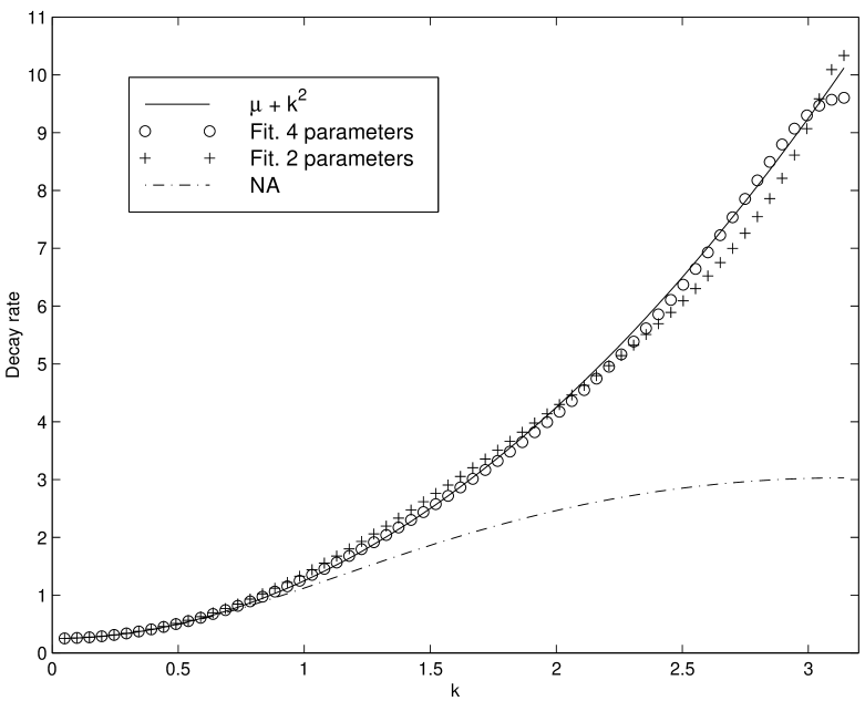
FIG. 15.: Decay rates of wave modes for the diffusion equation using the modified perfect operator. $\mu=0.25$, $\Delta t=\Delta x^{2}$.

For the MPO, the scaling regime starts from the first time node of the two point function (i.e. $S(k,t=0)$) due to the nearest neighbor interaction along the time direction. So long as the first two time nodes have reliable values, one can estimate the decay rate. This greatly loosens the precision constraint placed by the perfect operator used before. When the field has mass, direct fitting under modified constraints that take into account the mass cause little change in the coefficients.

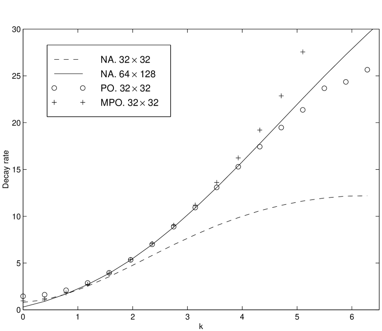
FIG. 16.: Decay rate of wave modes for the Ginzburg-Landau equation. $m=1$, $L=16$, $T=8$. The modified perfect operator gives results comparable to that of the perfect linear operator.

We tested the MPO in simulations of Model A dynamics. The results are comparable to that of the perfect operator (see Figure 16). It actually gives more accurate decay rates for wave modes at the edge of the first Brillouin zone, since it allows the use of the $t=0$ and $t=\Delta t$ nodes to compute the decay rate, while doing this for the PO is an approximation. The computational effort for the MPO is drastically reduced due to the relatively short interaction range.

The perfect linear operator operates on the coarse grained variable. For the modified perfect operator, the physical meaning of the variable it operates on is not apparent. As discussed in section I, there is a correspondence between an operator and a specific coarse graining scheme. For the local averaging CG scheme, or hard CG, the resulting perfect operator has a long interaction range. However, the range of interaction is reduced after we modify the CG scheme to be a soft CG scheme dependent on the parameter $\kappa$. Therefore, it is reasonable to think that there is a variant of the standard local averaging coarse graining scheme that gives the fast decaying operator we have computed above. The further investigation of this point is of general interest as regards the development of an efficient numerical algorithm.

VI Conclusions

The work presented in this paper is a first step towards reaping the full benefit of using renormalization group in the study of dynamics of spatially extended systems. We have constructed perfect representations of stochastic PDEs that not only integrate out the small scale degrees of freedom (in space and time), but also develop non-local representations of the underlying equations that are free of lattice artifacts. We demonstrated this by computing the dispersion relation for elementary excitations, and comparing the results at large wavenumbers with theoretical expressions valid in the continuum limit. We exhibited computations for diffusion equations, and a nonlinear equation derived from model A dynamics, and explored different ways to truncate the non-local space-time operators generated by the RG.

In one dimension, the computational complexity was reduced by a factor of about 40 from conventional simulations, for the simple diffusion problem. For the nonlinear model A equation, the results were less impressive, in terms of computer time, because a systematic approximation scheme for the perfect action has yet to be developed. Nevertheless, proceeding heuristically, we were still able to obtain improved results for the static structure factor and the decay rate of modes. Lastly, we proposed a heuristic discretization algorithm that incorporates the ideas of perfect operators, but also gives operators that are more local than perfect operators.

Finding the perfect operator when nonlinear interactions are present is a non-trivial task. The form of the continuous action is not closed under the CG transformation and new complicated interaction terms are generated. This is a general property of the RG[31]. Usually progress is only possible if the problem under consideration involves a small parameter which can be used to keep track of the new interactions which are generated. More generally, the small parameter allows a systematic approximation scheme to be developed, in which there is a clear prescription as to which terms have to be included at a given order. If such a parameter is not available, it is usual to fall back on to some type of variational scheme, typically including some kind of self-consistent calculation which corresponds to summing sets of diagrams. Neither of these approaches have been attempted in this paper. However, we feel that the results which we have obtained are sufficiently encouraging that some type of systematic calculation of the perfect operator in nonlinear theories would turn the ideas presented in this paper into a powerful computational tool.

A

In this appendix, we prove various relations that are important in deriving the iterative relations for perfect operators.

1. Here we list some properties of the projection matrices.

   We introduced $2N\times N$ matrices $\bar{\hat{R}}$, $\tilde{\hat{R}}$ and their left inverses $\bar{\hat{R}}^{-1}=\frac{1}{2}\bar{\hat{R}}^{T}$, $\tilde{\hat{R}}^{-1}=\frac{1}{2}\tilde{\hat{R}}^{T}$,

   $$\bar{\hat{R}}_{m,n}=\delta_{m,2n}+\delta_{m,2n-1},\ \ \tilde{\hat{R}}_{m,n}=\delta_{m,2n}+\delta_{m,2n-1}\ \ \ m\in[1,2N],\ \ n\in[1,N].$$ (A1)

   Here superscript $T$ indicates transposition. The projection matrices satisfy relations,

   $$\bar{\hat{R}}^{-1}\tilde{\hat{R}}=\tilde{\hat{R}}^{-1}\bar{\hat{R}}=0\ \ \mbox{ and }\ \ \bar{\hat{R}}\bar{\hat{R}}^{-1}+\tilde{\hat{R}}\tilde{\hat{R}}^{-1}=1\,.$$ (A2)

   We define the subscripted versions of $\hat{O}$ by

   $$\bar{\hat{R}}^{-1}\hat{O}\bar{\hat{R}}\equiv\hat{O}_{A}\tilde{\hat{R}}^{-1}\hat{O}\tilde{\hat{R}}\equiv\hat{O}_{B}\bar{\hat{R}}^{-1}\hat{O}\tilde{\hat{R}}\equiv\hat{O}_{C}\tilde{\hat{R}}^{-1}\hat{O}\bar{\hat{R}}\equiv\hat{O}_{D}\,,$$ (A3)

   where $\hat{O}$ and its subscripted versions are linear operators on the original grid and on the coarse grained grid respectively.

   One can prove the following formulae,

   $$g=\hat{O}f\Rightarrow\left\{\begin{array}[]{l}\bar{g}=(\bar{\hat{R}}^{-1}\hat{O}\bar{\hat{R}})\,\bar{f}+(\bar{\hat{R}}^{-1}\hat{O}\tilde{\hat{R}})\,\tilde{f}\equiv\hat{O}_{A}\,\bar{f}+\hat{O}_{C}\,\tilde{f}\\ \tilde{g}=(\tilde{\hat{R}}^{-1}\hat{O}\bar{\hat{R}})\,\bar{f}+(\tilde{\hat{R}}^{-1}\hat{O}\tilde{\hat{R}})\,\tilde{f}\equiv\hat{O}_{D}\,\bar{f}+\hat{O}_{B}\,\tilde{f}\end{array}\right.$$ (A6)

   $${f^{T}\hat{O}f}=2\,({\bar{f}^{T}\,\hat{O}_{A}\,\bar{f}+2\bar{f}^{T}\,\hat{O}_{C}\,\tilde{f}+\tilde{f}^{T}\,\hat{O}_{B}\,\tilde{f}})\ \ \mbox{ especially }\ \ f^{2}=2\,({\bar{f}}^{2}+{\tilde{f}}^{2})\,,$$ (A7)

   where we assumed that the matrix $\hat{O}$ is symmetric (physically, this means $\hat{O}$ possess inversion symmetry), and therefore $\hat{O}_{D}=\hat{O}_{C}^{T}$. Furthermore, if $\hat{O}$ is translational invariant with $\hat{O}_{m,n}={\hat{O}}_{m+i,n+i}$, $\hat{O}_{A}$ and $\hat{O}_{B}$ are symmetric while $\hat{O}_{C}$ and $\hat{O}_{D}$ are antisymmetric. This can be seen by looking at their elements,

   $$\left\{\begin{array}[]{ll}(\hat{O}_{A})_{m,n}&=\hat{O}_{2m,2n}+\frac{1}{2}(\hat{O}_{2m,2n+1}+\hat{O}_{2m,2n-1})\\ (\hat{O}_{B})_{m,n}&=\hat{O}_{2m,2n}-\frac{1}{2}(\hat{O}_{2m,2n+1}+\hat{O}_{2m,2n-1})\\ (\hat{O}_{C})_{m,n}&=\frac{1}{2}(\hat{O}_{2m,2n+1}-\hat{O}_{2m,2n-1})\,.\end{array}\right.\ \ \ m,n=1,\cdots,N.$$ (A11)

   In Fourier space, $\phi(m)=\sum\phi(k)\exp(ikm),\ \ m\in[1,2N]$ and $\bar{\phi}(n)=\sum\bar{\phi}(\kappa)\exp(i\kappa n),\ \ n\in[1,N]$. We have ${\bar{\hat{R}}}^{-1}=\frac{1}{2}\mathrm{c.c.}\,(\bar{\hat{R}}^{T})$, ${\bar{\hat{R}}}^{-1}=\frac{1}{2}\mathrm{c.c.}\,(\tilde{\hat{R}}^{T})$, where $\mathrm{c.c}$ is complex conjugate, and

   $$\left\{\begin{array}[]{l}{\bar{\hat{R}}}_{k,\kappa}=\sqrt{2}e^{i\frac{\kappa}{4}}(\cos\frac{\kappa}{4}\delta_{k,\frac{\kappa}{2}}-i\sin\frac{\kappa}{4}\delta_{k,\frac{\kappa}{2}\pm\pi})\\ {\tilde{\hat{R}}}_{k,\kappa}=\sqrt{2}e^{i\frac{\kappa}{4}}(-i\sin\frac{\kappa}{4}\delta_{k,\frac{\kappa}{2}}+\cos\frac{\kappa}{4}\delta_{k,\frac{\kappa}{2}\pm\pi})\end{array}\right.\ \ \ \kappa,k\in(-\pi,\pi).$$ (A14)

   The sign in $\frac{\kappa}{2}\pm\pi$ should be chosen so that its value lies within the interval $(-\pi,\pi)$. Physically, equation (A14) represents a two step process: folding of the Brillouin zone by half, such that two wave modes $k$ and $k\pm\pi$ are mixed, followed by a stretching back to $(-\pi,\pi)$. This is the corresponding process in Fourier space of the real space coarse graining transformation.

   Given the operator ${\hat{O}}=\sum O(k)|k\rangle\langle k|$, i.e. plane wave functions form its eigenspace, the coarse grained plane waves $|\kappa\rangle$ are also eigenvectors of ${\hat{O}}_{A}$, ${\hat{O}}_{B}$ and ${\hat{O}}_{C}$,

   $$\left\{\begin{array}[]{ll}(\hat{O}_{A})_{\kappa,\kappa^{\prime}}&=\delta_{\kappa,\kappa^{\prime}}[\cos^{2}\frac{\kappa}{4}O(\frac{\kappa}{2})+\sin^{2}\frac{\kappa}{4}O(\frac{\kappa}{2}\pm\pi)]\\ (\hat{O}_{B})_{\kappa,\kappa^{\prime}}&=\delta_{\kappa,\kappa^{\prime}}[\sin^{2}\frac{\kappa}{4}O(\frac{\kappa}{2})+\cos^{2}\frac{\kappa}{4}O(\frac{\kappa}{2}\pm\pi)]\\ (\hat{O}_{C})_{\kappa,\kappa^{\prime}}&=\delta_{\kappa,\kappa^{\prime}}(-i\cos\frac{\kappa}{4}\sin\frac{\kappa}{4})[O(\frac{\kappa}{2})-O(\frac{\kappa}{2}\pm\pi)]\end{array}\right.\ \ \ \kappa,\kappa^{\prime}\in(-\pi,\pi).$$ (A18)

2. In order to determine the iterative relations of linear operators (see 3 below), we first have to prove some properties of the subindexed matrices.

   • The first set of properties are:

     $$(\hat{O}^{-1})_{A}\cdot\hat{O}_{C} = -(\hat{O}^{-1})_{C}\cdot\hat{O}_{B}$$ (A19)

     $$\hat{O}_{D}\cdot(\hat{O}^{-1})_{A} = -\hat{O}_{B}\cdot(\hat{O}^{-1})_{D}$$ (A20)

     $$(\hat{O}^{-1})_{D}\cdot\hat{O}_{C} = 1-(\hat{O}^{-1})_{B}\cdot\hat{O}_{B}\,.$$ (A21)

     To prove the first relation, we use equation (A2):

     $$(\hat{O}^{-1})_{A}\cdot\hat{O}_{C} = \bar{\hat{R}}^{-1}\,\hat{O}^{-1}\,\bar{\hat{R}}\cdot\bar{\hat{R}}^{-1}\,\hat{O}\,\tilde{\hat{R}}=\bar{\hat{R}}^{-1}\,\hat{O}^{-1}\,(1-\tilde{\hat{R}}\,\tilde{\hat{R}}^{-1})\,\hat{O}\,\tilde{\hat{R}}$$ (A22)

     $$= \bar{\hat{R}}^{-1}\,\hat{O}^{-1}\,\hat{O}\,\tilde{\hat{R}}-\bar{\hat{R}}^{-1}\,\hat{O}^{-1}\,\tilde{\hat{R}}\,\tilde{\hat{R}}^{-1}\,\hat{O}\,\tilde{\hat{R}}$$ (A23)

     $$= \bar{\hat{R}}^{-1}\,\tilde{\hat{R}}-(\hat{O}^{-1})_{C}\,\hat{O}_{B}=-(\hat{O}^{-1})_{C}\,\hat{O}_{B}\,.$$ (A24)

     We can prove the other two relations in a similar way.

   • Another very useful result is:

     $$(\hat{O}^{-1})_{A}=(\hat{O}_{A}-\hat{O}_{C}(\hat{O}_{B})^{-1}\hat{O}_{D})^{-1}$$ (A25)

     We prove this using equations (A21):

     $$(\hat{O}^{-1})_{A}\cdot(\hat{O}_{A}-\hat{O}_{C}(\hat{O}_{B})^{-1}\hat{O}_{D}) = (\hat{O}^{-1})_{A}\cdot\hat{O}_{A}+(\hat{O}^{-1})_{C}\,\hat{O}_{D}$$ (A26)

     $$= \bar{\hat{R}}^{-1}\,\hat{O}^{-1}\,\bar{\hat{R}}\,\bar{\hat{R}}^{-1}\,\hat{O}\,\bar{\hat{R}}+\bar{\hat{R}}^{-1}\,\hat{O}^{-1}\,\tilde{\hat{R}}\,\tilde{\hat{R}}^{-1}\,\hat{O}\,\bar{\hat{R}}$$ (A27)

     $$= \bar{\hat{R}}^{-1}\,\hat{O}^{-1}\,\hat{O}\,\bar{\hat{R}}$$ (A28)

     $$= \bar{\hat{R}}^{-1}\,\bar{\hat{R}}=1$$ (A29)

3. The iterative relation for the action operator (equation (24)) follows from that of $\rho$ (equation (17)) which reads

   $$(\hat{\rho^{CG}})^{-1}=\hat{L}_{C}\hat{M}^{-1}\hat{\rho}_{B}^{-1}(\hat{M}^{-1})^{T}\hat{L}^{T}_{C}+\hat{\Gamma}\,(\hat{\rho}_{A}-\hat{\rho}_{C}\hat{\rho}_{B}^{-1}\hat{\rho}_{D})^{-1}\,\hat{\Gamma}^{T}\,,$$ (A30)

   where $\hat{\Gamma}=\hat{I}+\hat{O}_{C}(\hat{O}_{B})^{-1}\hat{\rho}_{B}^{-1}\hat{\rho}_{D}$, and where we use $\hat{O}$ to denote the full dynamic evolution operator $\hat{L}_{\omega}$. Since $\rho$ is symmetric, $A$ and $B$ subindexed matrices are symmetric while $C$ subindexed matrix is the transpose of $D$ subindexed matrix. Using equations (A21) and (A25), the second term in the above equation yields,

   $$\hat{\Gamma}\,(\hat{\rho}^{-1})_{A}\,\hat{\Gamma}^{T} = (\hat{\rho}^{-1})_{A}-\hat{O}_{C}(\hat{O}_{B})^{-1}\,(\hat{\rho}^{-1})_{D}-(\hat{\rho}^{-1})_{C}\,(\hat{O}^{T}_{B})^{-1}\hat{O}_{C}^{T}$$ (A32)

   $$+\hat{O}_{C}(\hat{O}_{B})^{-1}\,\left[(\hat{\rho}^{-1})_{B}-(\hat{\rho}_{B})^{-1}\right]\,(\hat{O}^{T}_{B})^{-1}\hat{O}_{C}^{T}\,.$$

   Therefore (if for the US scheme, ignore the factor of 2),

   $$(\hat{\rho}^{M})^{-1} = (\hat{\rho}^{-1})_{A}+\hat{O}_{C}(\hat{O}^{-1})_{B}\,(\hat{\rho}^{-1}_{B})\,(\hat{O}^{T}_{B})^{-1}\hat{O}_{C}^{T}$$ (A34)

   $$-\hat{O}_{C}(\hat{O}_{B})^{-1}\,(\hat{\rho}^{-1})_{D}-(\hat{\rho}^{-1})_{C}\,(\hat{O}^{T}_{B})^{-1}\hat{O}_{C}^{T}\,.$$

   Therefore, using the iterative relation $(\hat{O}^{M})^{-1}=(\hat{O}^{-1})_{A}$ and equations (A21), we have,

   $$(\hat{O}^{M})^{-1}\,(\hat{\rho}^{M})^{-1}\,(\hat{O}^{M})^{T}\,{}^{-1}$$ (A35)

   $$= (\hat{O}^{-1})_{A}\,(\hat{\rho}^{-1})_{A}\,(\hat{O}^{T}\,{}^{-1})_{A}+(\hat{O}^{-1})_{A}\,\hat{O}_{C}(\hat{O}_{B})^{-1}\,(\hat{\rho}^{-1})_{B}\,(\hat{O}^{T}_{B})^{-1}\hat{O}_{C}^{T}\,(\hat{O}^{T}\,{}^{-1})_{A}$$ (A37)

   $$-(\hat{O}^{-1})_{A}\,\hat{O}_{C}(\hat{O}_{B})^{-1}\,(\hat{\rho}^{-1})_{D}\,(\hat{O}^{T}\,{}^{-1})_{A}-(\hat{O}^{-1})_{A}\,(\hat{\rho}^{-1})_{C}\,(\hat{O}^{T}_{B})^{-1}\hat{O}_{C}^{T}\,(\hat{O}^{T}\,{}^{-1})_{A}$$

   $$= (\hat{O}^{-1})_{A}\,(\hat{\rho}^{-1})_{A}\,(\hat{O}^{T}\,{}^{-1})_{A}+(\hat{O}^{-1})_{C}\,(\hat{\rho}^{-1})_{B}\,(\hat{O}^{T}\,{}^{-1})_{C}$$ (A39)

   $$+(\hat{O}^{-1})_{C}\,(\hat{\rho}^{-1})_{D}\,(\hat{O}^{T}\,{}^{-1})_{A}+(\hat{O}^{-1})_{A}\,(\hat{\rho}^{-1})_{C}\,(\hat{O}^{T}\,{}^{-1})_{C}\,.$$

   On the other hand, we have

   $$(\hat{O}^{-1}\,\hat{\rho}^{-1}\,\hat{O}^{T}\,{}^{-1})_{A} = \bar{\hat{R}}^{-1}\,\hat{O}^{-1}\,(\bar{\hat{R}}\,\bar{\hat{R}}^{-1}+\tilde{\hat{R}}\,\tilde{\hat{R}}^{-1})\,\hat{\rho}^{-1}\,(\bar{\hat{R}}\,\bar{\hat{R}}^{-1}+\tilde{\hat{R}}\,\tilde{\hat{R}}^{-1})\,\hat{O}^{T}\,{}^{-1}\,\bar{\hat{R}}\,.$$ (A40)

   Expanding the above equation and comparing with equation (A39), proves equation (24).

REFERENCES

- [1] N. Goldenfeld, A. McKane and Q. Hou, J. Stat. Phys. 93, 699 (1998).
- [2] A. J. Chorin, A. Kast and R. Kupferman, Proc. Nat. Acad. Sci. USA, 95, 4094 (1998).
- [3] A. J. Chorin, A. Kast and R. Kupferman, Comm. Pure. Appl. Math. 52, 1231 (1999).
- [4] A. J. Chorin, R. Kupferman and D. Levy, J. Comput. Phys. 162, 267 (2000).
- [5] A. J. Chorin, O. H. Hald and R. Kupferman, Proc. Nat. Acad. Sci. USA 97, 2968 (2000).
- [6] J. Bell, A. J. Chorin and W. Crutchield, Stochastic Optimal Prediction with Application to Averaged Euler Equations. Available at http://www.lbl.gov/chorin.
- [7] J. A. Langford and R. D. Moser, J. Fluid. Mech. 398, 321 (1999).
- [8] P. Hasenfratz, Prog. Theor. Phys. Supp. 131, 189 (1998).
- [9] E. Katz and U.-J. Wiese, Phys. Rev. E58, 5796 (1998).
- [10] S. Hauswirth, Perfect discretizations of differential operators, hep-lat/0003007.
- [11] For a review, see Y. Oono and A. Shinozaki, Forma 4, 75 (1989).
- [12] A. Shinozaki and Y. Oono, Phys. Rev. E48, 2622 (1993).
- [13] M. Mondello and N. Goldenfeld, Phys. Rev. A [Rapid Commun.] 42, 5865 (1990); ibid. Phys. Rev. A 45, 657 (1992).
- [14] M. Zapotocky, P. M. Goldbart and N. D. Goldenfeld, Phys. Rev. E 51, 1216 (1995).
- [15] M.D. Lacasse, J. Vinals and M. Grant, Phys. Rev. B47, 5646 (1993).
- [16] B. Grossman, H. Guo and M. Grant, Phys. Rev. E41, 4195 (1990).
- [17] This diagram suggests that coarse-graining and time evolution commute. This is not true for cases of chaotic dynamics[1].
- [18] J. Zinn-Justin, Quantum Field Theory and Critical Phenomena (OUP, New York, 1996).
- [19] A.J. McKane, H.C. Luckock and A.J. Bray, Phys. Rev. 41, 644 (1990).
- [20] T.L. Bell and K. Wilson, Phys. Rev. B10, 3935 (1974).
- [21] K.G. Wilson, in New Pathways in High Energy Physics II (Plenum, New York, 1976) page 243.
- [22] P. Hasenfratz and F. Niedermayer, Nucl. Phys. B414, 785 (1994).
- [23] Q. Hou, unpublished.
- [24] M. Zimmer, Phys. Rev. Lett. 75, 1431 (1995).
- [25] Here a operator means it has independent elements. Mirror symmetry with respect to the axis gives us the other elements in the operator. Along each axis, there are at most and neighbors.
- [26] W. Bietenholz, Perfect and Quasi-Perfect Lattice Actions, hep-lat/9802014.
- [27] W. Bietenholz and H. Dilger, Nucl. Phys. B549, 335 (1999); Nucl. Phys. B (Proc. Suppl.) 73, 933 (1999).
- [28] K. Binder (Ed) The Monte Carlo method in condensed matter physics (Springer-Verlag, Berlin, 1995).
- [29] W.H. Press, S.A. Teukolsky, W.T. Vetterling and B.P. Flannery, Numerical Recipes in C: the art of scientific computing (CUP, New York, 1992).
- [30] D. Ceperley, M. Mascagni and A. Srinivasan, http://www.ncsa.uiuc.edu/Apps/SPRNG.
- [31] N. Goldenfeld, Lectures on Phase Transitions and the Renormalization Group (Addison-Wesley, Reading, Mass., 1992).