Charge Fluctuations in the Single Electron Box

Abstract

Quantum fluctuations of the charge in the single electron box are investigated. Based on a diagrammatic expansion we calculate the average island charge number and the effective charging energy in third order in the tunneling conductance. Near the degeneracy point where the energy of two charge states coincides, the perturbative approach fails, and we explicitly resum the leading logarithmic divergencies to all orders. The predictions for zero temperature are compared with Monte Carlo data and with recent renormalization group results. While good agreement between the third order result and numerical data justifies the perturbative approach in most of the parameter regime relevant experimentally, near the degeneracy point and at zero temperature the resummation is shown to be insufficient to describe strong tunneling effects quantitatively. We also determine the charge noise spectrum employing a projection operator technique. Former perturbative and semiclassical results are extended by the approach.

I Introduction

Tunneling of electrons in metallic nanostructures is strongly affected by Coulomb repulsion. Provided the screening length in the metallic films is small compared to tunneling barrier thickness and sample size, the Coulomb energy can be written in terms of a geometrical capacitance $C$. The relevant energy scale of the system is the corresponding charging energy $E_{C}=e^{2}/2C$ [1] that is the energy needed to charge the capacitance $C$ by one electron. For temperatures well below this energy, $k_{B}T\ll E_{C}$, tunneling onto a metallic island is exponentially suppressed. For weak tunneling strength, $G_{T}\ll G_{K}$, where $G_{T}$ is the phenomenological tunneling conductance and $G_{K}=e^{2}/h$ the conductance quantum, systems are well described by the perturbative approach in $\alpha=G_{T}/G_{K}$ [2, 3]. When the tunneling conductance becomes larger, higher orders in the perturbative series in $\alpha$ such as cotunneling [4] have to be included. Even at zero temperature these processes are not forbidden energetically, therefore, higher order corrections are most pronounced at low temperatures where first order processes are exponentially suppressed. Due to the large number of terms in the perturbative series, the approach remains restricted to the first few orders in $\alpha$ and one is interested in the range of validity one could expect. At higher temperatures, $k_{B}T\gg E_{C}$, thermal fluctuations dominate and perturbation theory (PT) becomes more accurate. Therefore, to give a lower bound of the validity of PT it is sufficient to consider the zero temperature case where PT is worst. In fact, PT at zero temperature even diverges at the degeneracy point of the single electron box (SEB) showing that the range of validity depends on both, tunneling strength and applied gate voltage.

While partial resummation techniques [5, 6, 7, 8] lead to a nonperturbative finite result even at the degeneracy point, they need an arbitrary cutoff that limits their use for direct comparison with experiments. Recently, renormalization group (RG) ideas [9] have been used to remove the cutoff yielding results that depend on parameters measurable experimentally. On the other hand, a complete resummation of PT can be achieved in phase representation leading to a formally exact path integral formulation of single electron devices [10, 11]. Here, the phase is the conjugate operator to the island charge number and can be related to the physical voltage drop across the junction. The functional can serve as starting point for analytical predictions in the semiclassical limit [12, 13, 14, 15, 16, 17, 18, 19] covering the range of high temperatures and/or large conductance. It also is the basis of numerical calculations [20, 21, 22, 23].

In this paper we study the single electron box by systematic diagrammatic techniques. So far PT for any temperature has been calculated to the first and the second orders in $\alpha$ [24]. Here, we determine the third order corrections at zero temperature and compare them with Monte-Carlo (MC) results [20, 21, 22, 25] and recent RG data [26]. Further, we explicitly address the vicinity of the degeneracy point where PT fails and derive a nonperturbative result by resummation of graphs contributing to the leading logarithmical divergencies. We also discuss the charge noise spectrum nonperturbatively by means of a projection operator technique. In general, the spectrum depends on the electronic bandwidth, however, for frequencies relevant experimentally only the high frequency cutoff characterizing the resolution of the measuring device matters.

The paper is organized as follows: In Sec. II we introduce the system Hamiltonian and the average island charge number. In Sec. III we briefly recapitulate essential results and diagrammatic rules of the perturbative expansion [24]. The necessary changes and simplifications in the zero temperature limit are given in Sec. IV where we exemplarily evaluate one graph of third order. In Sec. V we present the analytic result for the average charge number. The two state approximation and the resummation of the leading logarithmical divergencies at the degeneracy point are discussed in Sec. VI. In Sec. VII we compare the analytical findings for the average island charge number and the effective charging energy with MC data and recent RG results. Finally, in Sec. VIII we determine the noise spectrum of the island charge number and conclude in Sec. IX.

II System and Model Hamiltonian

We consider a SEB consisting of a metallic grain that couples to a lead electrode via an oxide layer. The separation permits tunneling of single electrons with the corresponding phenomenological tunneling conductance $G_{T}$. The geometrical capacitance between the grain an the lead reads $C_{T}$. Furthermore, a gate electrode is capacitively coupled to the grain with gate capacitance $C_{g}$. This setup is shown schematically in Fig. 1, where the circuit is biased by a gate voltage $U_{g}$ shifting the Coulomb energy continuously. We describe the SEB by the Hamiltonian [24]

$$H=H_{0}+H_{T}$$ (1)

where

$$H_{0}=H_{C}+H_{\rm qp}$$ (2)

represents the system in absence of tunneling. Here,

$$H_{\rm qp}=\sum_{k\sigma}\epsilon_{k\sigma}a^{\dagger}_{k\sigma}a_{k\sigma}+\sum_{q\sigma}\epsilon_{q\sigma}a^{\dagger}_{q\sigma}a_{q\sigma}$$ (3)

describes free Fermions where the quasiparticle creation and annihilation operators for transversal and spin quantum number $\sigma$ and longitudinal quantum number $p=k,q$ for the island and the lead electrode, respectively, are denoted by $a^{\dagger}_{p\sigma}$ and $a_{p\sigma}$. Further, $\epsilon_{p\sigma}$ are quasiparticle energies for the corresponding quantum numbers.

$$H_{C}=E_{C}(n-n_{g})^{2}$$ (4)

is the Coulomb energy for $n$ excess charges on the island biased by the dimensionless external voltage $n_{g}=C_{g}U_{g}/e$. The charging energy

$$E_{C}=\frac{e^{2}}{2C}$$ (5)

depends solely on the island capacitance $C=C_{T}+C_{g}$. Spin and transversal quantum numbers are conserved during the tunneling process described by the tunneling Hamiltonian

$$H_{T}=\sum_{kq\sigma}\left(t_{kq\sigma}a^{\dagger}_{k\sigma}a_{q\sigma}\Lambda+\mbox{H.c.}\right),$$ (6)

with $t_{kq\sigma}$ the transition amplitude between states with quantum numbers $k\sigma$ and $q\sigma$. The charge shift operator $\Lambda$ accounts for the Coulomb energy and is related to the charge number operator $n$ by the relation

$$\Lambda^{\dagger}n\Lambda=n+1.$$ (7)

FIG. 1.: Circuit diagram of a single electron box.

The excess charge number $n$ can be expressed as a derivative of the system Hamiltonian with respect to $n_{g}$. Accordingly, we find for the average island charge number

$$\langle n\rangle=n_{g}+\frac{1}{2\beta E_{c}}~{}\frac{\partial\ln Z}{\partial n_{g}}~{}~{},$$ (8)

where

$$Z={\rm tr}\{\exp(-\beta H)\}$$ (9)

is the partition function of the system. At low temperatures and in the limit of vanishing tunneling conductance the logarithm of the partition function reduces to the minimum of the electrostatic energy $E_{C}(n_{0}-n_{g})^{2}$ where $n_{0}$ is the integer closest to $n_{g}$. Hence, as a function of the applied voltage $U_{g}$ the island charge number displays the well known Coulomb staircase $\langle n\rangle=n_{0}$ observed experimentally [27]. Due to occupation of higher energy levels at finite temperatures the step function is smeared. Similarly, the Coulomb staircase is rounded by virtual occupation of higher charge levels caused by the finite tunneling conductance. Here, we restrict ourselves to zero temperature and discuss the influence of higher order tunneling processes on charge fluctuations. Because of the periodicity and symmetry of the partition function $Z$ with respect to $n_{g}$, it is sufficient to consider $0\leq n_{g}<\scriptstyle{\frac{1}{2}}$.

III Perturbation Expansion and Diagrammatic Rules

In this section we briefly summarize the method in Ref. [24] and give the diagrammatic rules used in the remainder.

A Perturbation Expansion

Since the $n_{g}$ dependence of the partition function $(\ref{eq:ParitionGen})$ arises from the charging energy only, we may put

$$Z:=\frac{{\rm tr}\,e^{-\beta H}}{{\rm tr}_{\rm qp}\,e^{-\beta H_{\rm qp}}}\,.$$ (10)

Factorizing the exponential $\exp(-\beta H)$ into a part $\exp(-\beta H_{0})$ in the absence of tunneling and an interaction part written as a series in the tunneling Hamiltonian $H_{T}$ we get

$$Z = \sum_{m=0}^{\infty}(-1)^{m}\int_{0}^{\beta}d\alpha_{m}\int_{0}^{\alpha_{m}}d\alpha_{m-1}\ldots\int_{0}^{\alpha_{2}}d\alpha_{1}\,$$ (12)

$$\frac{{\rm tr}\left\{e^{-\beta H_{0}}H_{T}(\alpha_{m})\ldots H_{T}(\alpha_{1})\right\}}{{\rm tr}_{\rm qp}\,e^{-\beta H_{\rm qp}}}\,,$$

with the tunneling Hamiltonian in imaginary time interaction picture

$$H_{T}(\tau)=e^{\tau H_{0}}H_{T}e^{-\tau H_{0}}\,.$$ (13)

Separating the trace in a Coulomb and a quasiparticle trace

$${\rm tr}\,e^{-\beta H_{0}}\ldots={\rm tr}_{C}\,e^{-\beta H_{C}}\,{\rm tr}_{\rm qp}\,e^{-\beta H_{\rm qp}}\ldots$$ (14)

one is left with multi-point correlation functions of tunneling Hamiltonians in imaginary time

$$Z = \sum_{m=0}^{\infty}(-1)^{m}\int_{0}^{\beta}d\alpha_{m}\int_{0}^{\alpha_{m}}d\alpha_{m-1}\ldots\int_{0}^{\alpha_{2}}d\alpha_{1}\,$$ (16)

$${\rm tr}_{C}\,e^{-\beta H_{C}}\,\langle H_{T}(\alpha_{m})\ldots H_{T}(\alpha_{1})\rangle_{0}\,,$$

where

$$\langle X\rangle_{0}=\frac{{\rm tr}_{\rm qp}\left\{e^{-\beta H_{\rm qp}}\,X\right\}}{{\rm tr}_{\rm qp}\,e^{-\beta H_{\rm qp}}}$$ (17)

is the thermal quasiparticle average. Due to the Coulomb interaction these correlators do not decompose into a product of two-point correlators. However, inserting the explicit form $(\ref{eq:tunnelHamil})$ of $H_{T}$, the charge shift operators in interaction picture $\Lambda(\tau)=\exp(\tau H_{C})\Lambda\exp(-\tau H_{C})$ commute with the quasiparticle operators and therefore may be factored out of the quasiparticle trace leading to

$$Z = \sum_{m=0}^{\infty}(-1)^{m}\int_{0}^{\beta}d\alpha_{m}\int_{0}^{\alpha_{m}}d\alpha_{m-1}\ldots\int_{0}^{\alpha_{2}}d\alpha_{1}$$ (21)

$$\sum_{k_{1}q_{1}\sigma_{1}\zeta_{1}}\ldots\sum_{k_{m}q_{m}\sigma_{m}\zeta_{m}}t^{m}\zeta_{1}\ldots\zeta_{m}$$

$$\sum_{n=-\infty}^{\infty}e^{-\sum_{j=1}^{2m}(\alpha_{j}-\alpha_{j-1})E_{n_{j}}}$$

$$\left\langle a_{k_{m}\sigma_{m}}^{\zeta_{m}}(\alpha_{m})a_{q_{m}\sigma_{m}}^{-\zeta_{m}}(\alpha_{m})\ldots a_{k_{1}\sigma_{1}}^{\zeta_{1}}(\alpha_{1})a_{q_{1}\sigma_{1}}^{-\zeta_{1}}(\alpha_{1})\right\rangle_{0}\,.$$

Here, the Coulomb trace is explicitly represented as a sum over charge states labeled by $n$ and

$$E_{n}=E_{C}(n-n_{g})^{2}$$ (22)

is the corresponding Coulomb energy. The charge shift operators in interaction picture lead to exponentials $\exp[\alpha_{j}(E_{n_{j+1}}-E_{n_{j}})]$ where the integers $n_{j}$ are defined by

$$n_{1}=n,\qquad\quad n_{j}=\sum_{k=1}^{j-1}\zeta_{k}\,,$$ (23)

with $\zeta_{k}=\pm$ labeling excess charge number increasing or decreasing processes. Due to charge conservation the $\zeta$ sums in Eq. $(\ref{eq:boxIIpartfkt})$ are constrained by

$$\sum_{j=1}^{2m}\zeta_{j}=0\,.$$ (24)

Further, we have introduced the shorthand notation $a^{+}=a^{\dagger}$ and $a^{-}=a$, respectively, and $t=\overline{t_{kq\sigma}}$ is a real averaged transmission amplitude. Now time difference variables $\beta_{j}$, $(j=1,\ldots,2m)$ between two subsequent operators are introduced and the cyclic invariance of the trace can be used to obtain

$$Z = \sum_{m=0}^{\infty}\frac{\beta}{2m}t^{2m}\int_{0}^{\infty}d\beta_{1}\cdots\int_{0}^{\infty}d\beta_{2m}\delta\!\left(\sum_{j=1}^{2m}\beta_{j}-\beta\right)$$ (27)

$$\sum_{\zeta_{1},\ldots,\zeta_{2m}}\sum_{n=-\infty}^{\infty}e^{-\sum_{j=1}^{2m}\beta_{j}E_{n_{j}}}\sum_{k_{1}q_{1}\sigma_{1}}\cdots\sum_{k_{2m}q_{2m}\sigma_{2m}}$$

$$\left\langle\prod_{j=1}^{2m}\zeta_{j}a_{k_{j}\sigma_{j}}^{\zeta_{j}}\!\left(\sum_{l=1}^{j}\beta_{l}\right)a_{q_{j}\sigma_{j}}^{-\zeta_{j}}\!\left(\sum_{l=1}^{j}\beta_{l}\right)\right\rangle_{0}\,.$$

Since the free quasiparticle Hamiltonian $H_{\rm qp}$ is quadratic in the fermionic degrees of freedom, the expectations of quasiparticle operators $a^{\dagger}_{p\sigma}(\tau)$ and $a_{p\sigma}(\tau)$ obey a Wick theorem and the average in $(\ref{eq:partition1})$ decomposes into a sum over pair products of two-point correlators

$$\left\langle a_{p_{1}\sigma_{1}}^{\zeta_{1}}(\tau_{1})a_{p_{2}\sigma_{2}}^{\zeta_{2}}(\tau_{2})\right\rangle_{0}=\delta_{\zeta_{1},-\zeta_{2}}\delta_{p_{1},p_{2}}\delta_{\sigma_{1},\sigma_{2}}\frac{e^{\zeta_{1}(\tau_{1}-\tau_{2})\epsilon_{p_{1}\sigma_{1}}}}{1+e^{\zeta_{1}\beta\epsilon_{p_{1}\sigma_{1}}}}.$$ (28)

So far the result is valid for arbitrary numbers of tunneling channels

$${\cal N}=\sum_{\sigma}1.$$ (29)

In metallic junctions where the junction area is typically much larger than the Fermi wavelength squared, ${\cal N}$ is very large. Experimentally the value is of the order ${\cal N}\approx 10^{4}$ justifying limiting considerations.

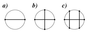
FIG. 2.: Representative circle diagrams of a) first, b) second, and c) third order in the perturbative series.

The $1/{\cal N}$ corrections for the SEB are considered explicitly in Ref. [28] confirming the validity of the approximation. In leading order only the combination

$$\!\!\!\!\!\!Y(\tau_{2}-\tau_{1})$$ (30)

$$= t^{2}\sum_{k_{1}q_{1}k_{2}q_{2}\sigma}\langle a^{\zeta}_{k_{2}\sigma}(\tau_{2})a^{-\zeta}_{k_{1}\sigma}(\tau_{1})\rangle_{0}\langle a^{-\zeta}_{q_{2}\sigma}(\tau_{2})a^{\zeta}_{q_{1}\sigma}(\tau_{1})\rangle_{0}$$ (31)

$$= g\int_{-\infty}^{\infty}d\epsilon\frac{\epsilon e^{-|\epsilon|/D}}{1-e^{-\beta\epsilon}}e^{-(\tau_{2}-\tau_{1})\epsilon}$$ (32)

of two two-point correlators contributes. Here, we have replaced the sums over $k$ and $q$ by energy integrals and have already performed one of them. We introduced the notation $g=t^{2}{\cal N}\rho\rho^{\prime}=\alpha/4\pi^{2}$ where $\rho$ and $\rho^{\prime}$ are densities of states at the Fermi level for the island and the lead electrode, respectively. The function $Y(\tau)$ is an electron-hole pair Green function where electron and hole are created in different electrodes and $D$ is the electronic bandwidth. Representing the $\delta$-function in Eq. $(\ref{eq:partition1})$ in terms of an energy integral over an auxiliary variable $E$

$$\delta(\tau)=\frac{1}{2\pi}\int dEe^{-i\tau E}\,,$$ (33)

one can perform all imaginary time integrals $\beta_{j}$, $(j=1\ldots 2m)$ gaining energy denominators that are linear combinations of the auxiliary variable $E$ as well as $E_{n_{j}}$, $(j=1\ldots 2m)$ and $\epsilon_{k}$, $(k=1\ldots m)$. The coefficients of the linear combinations depend on the Wick decomposition and the $\zeta$-sums in $(\ref{eq:partition1})$. The remaining summations over pairs and $\zeta_{j}$’s can be represented graphically by diagrams, in terms of which the partition function reads

$$Z=\frac{1}{2\pi}\int_{-\infty}^{\infty}dE\,e^{i\beta E}\sum_{\rm diagrams}D(E)\,.$$ (34)

In Fig. 2 representative circle diagrams of a) first, b) second, and c) third order in PT are shown. A diagram $D(E)$ includes the charge sum $\sum_{n=-\infty}^{\infty}$ and each circle segment correspond to an energy denominator

$$\frac{1}{E_{n_{j}}+\sum_{k=1}^{m}\Theta_{jk}\epsilon_{k}+iE}$$ (35)

where $\Theta_{jk}=1$ for a time interval $\beta_{j}$ in between of two vertices connected by a straight tunnelon line, and $\Theta_{jk}=0$ otherwise. The tunnelon lines represent energy integrals

$$g\int d\epsilon_{k}\frac{\epsilon_{k}e^{-|\epsilon_{k}|/D}}{1-e^{-\beta\epsilon_{k}}}$$ (36)

for $k=1,\ldots,m$, stemming from electron-hole pair Green functions $(\ref{eq:greensf})$. Since with respect to the auxiliary variable $E$ the whole integrand is a product of energy denominators, the integral can be performed explicitly by means of contour integration.

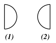
FIG. 3.: Diagrams of first order in the perturbative series.

One gains a sum over residua corresponding to poles at a certain circle segment. Since residua of higher order poles correspond to derivatives of the product of finite energy denominators with respect to $E$, we get graphs decorated by slashes. The decorations are placed on the finite segments indicating a derivative of the corresponding energy denominator with respect to the auxiliary variable $E$ evaluated at the pole position considered. The simple form of the energy denominators allows us to perform the derivatives explicitly. We gain a higher power of the energy denominator $1/{\cal E}^{q+1}$ times $(-i)^{q}q!$ for a $q$-fold derivative of $1/{\cal E}$. This way the sum over residua can be represented by circle diagrams, where the divergent circle segments are omitted and the remaining finite segments are decorated with slashes indicating derivatives of the energy denominator evaluated at the pole position. Considering a circle diagram with a pole of order $r$, one finds that when the pole segments are omitted, the graph decomposes into $r$ pieces denoted by $T_{q}$ with $q=1,\ldots,r$. The partition function may then be arranged according to the order of poles

$$Z=\sum_{r=1}^{\infty}{\sum_{\rm diag}}^{r}\sum_{n=-\infty}^{\infty}e^{-\beta E_{n}}\sum_{s=0}^{r-1}\frac{\beta^{r-s}}{(r-s-1)!}\frac{1}{f}\left[\prod_{q=1}^{r}T_{q}\right]^{(s)}$$ (37)

where the sum over diagrams is restricted to those with poles of order $r$ and the symbol $[\ldots]^{(s)}$ stands for the sum over all decorations (derivatives) between the brackets with $s$ slashes. Further, the factor $f$ is the number of identical subgroups in $T_{q}$, $q=1,\ldots,r$. Introducing the quantity

$$U_{r}^{(s)}={\sum_{\rm diag}}^{r}\left[\prod_{q=1}^{r}T_{q}\right]^{(s)}$$ (38)

we may write the partition function in the form

$$Z=\sum_{n=-\infty}^{\infty}e^{-\beta E_{n}}\left\{1+\sum_{p=1}^{\infty}\frac{\beta^{p}}{p!}\sum_{s=0}^{\infty}\frac{p}{p+s}U_{p+s}^{(s)}\right\}\,.$$ (39)

Using analytical properties of $U_{r}^{(s)}$ one may show that [24]

$$\sum_{s=0}^{\infty}\frac{p}{p+s}U_{p+s}^{(s)}=\left(\sum_{s=0}^{\infty}\frac{1}{s+1}U_{s+1}^{(s)}\right)^{p}\,.$$ (40)

This way one gets an effective Coulomb representation of the partition function

$$Z=\sum_{n=-\infty}^{\infty}e^{-\beta(E_{n}+\Delta_{n})},$$ (41)

where

$$\Delta_{n}=-\sum_{r=1}^{\infty}\,{\sum_{\rm diag}}^{r}\,\frac{1}{r}\left[\prod_{q=1}^{r}\,T_{q}\right]^{(r-1)}$$ (42)

is the energy correction to the Coulomb energy of state $n$ that may be written

$$\Delta_{n}=\sum_{m=1}^{\infty}\Delta_{n}^{(m)}\,,$$ (43)

where $\Delta_{n}^{(m)}$ is the contribution of order $g^{m}$.

B Diagrammatic Rules for $\Delta_{n}^{(m)}$

In this subsection we give the diagrammatic rules for the energy corrections $(\ref{eq:energycorr})$. The term of order $g^{m}$ is given by $\Delta_{n}^{(m)}$ and is composed of graphs containing a vertical line with $m$ semicircles attached. Each semicircle corresponds to a tunneling event and represents an energy integral

$$g\int_{-\infty}^{\infty}d\epsilon\frac{\epsilon e^{-|\epsilon|/D}}{1-e^{-\beta\epsilon}}$$ (44)

stemming from the electron-hole pair Green function $(\ref{eq:greensf})$. Further each vertical line element contributes an energy denominator $\,-1/{\cal E}$ where ${\cal E}$ is the excitation energy during the corresponding intermediate state, which is the sum of the Coulomb energy difference

$$\xi_{p}=E_{n+p}-E_{n}$$ (45)

and of all electron-hole pair excitation energies $\epsilon_{j}$ present in the intermediate state that are represented by the arcs that would be intersected by a horizontal line. There are two types of semicircles: inflected to the right or left, whereby the Coulomb state $n$ is increased (decreased) by an arc to the right (left). For example in first order in $g$ there are just two processes depicted in Fig. 3. Whereas the graph $(1)$ increases the excess charge number by one and therefore represents

$$\Delta_{n}^{(1,1)}=-g\int_{-\infty}^{\infty}d\epsilon\frac{\epsilon e^{-|\epsilon|/D}}{1-e^{-\beta\epsilon}}\frac{1}{\xi_{1}+\epsilon}\,,$$ (46)

the graph $(2)$ lowers the charge number and it’s contribution $\Delta_{n}^{(1,2)}$ is obtained from the previous one by replacing $\xi_{1}\rightarrow\xi_{-1}$.

FIG. 4.: Diagrams of second order.

In second order, cf. Fig. 4, there are two semicircles dividing the vertical line into three parts. Each of them represents an energy denominator at the corresponding charging energy. The graphs $(1)$ to $(8)$ in Fig. 4 are given by all possibilities to attach two semicircles to a vertical line. Using the rules given above the graph $(1)$ in Fig. 4 correspond to

$$\Delta_{n}^{(2,1)} = -g^{2}\int_{-\infty}^{\infty}d\epsilon_{1}\int_{-\infty}^{\infty}d\epsilon_{2}\frac{\epsilon_{1}e^{-|\epsilon_{1}|/D}}{1-e^{-\beta\epsilon_{1}}}\frac{\epsilon_{2}e^{-|\epsilon_{2}|/D}}{1-e^{-\beta\epsilon_{2}}}$$ (48)

$$\frac{1}{(\xi_{1}+\epsilon_{1})^{2}}\frac{1}{\xi_{2}+\epsilon_{1}+\epsilon_{2}}$$

representing two tunneling processes with three intermediate energy denominators. Since an arc to the left hand side represents a tunneling process that lowers the charge number on the island, the contribution of graph $(2)$ differs from that of graph $(1)$ by the replacement $\xi_{2}\rightarrow 0$. The first eight graphs in Fig. 4 can be generated easily by the rules given. The graphs $(9)$ to $(12)$, however, differ by the prolongation of the interior arcs across the vertical line. These “insertions” represent separate graphs, i.e. each insertion represents a graph of lower order multiplied to the main graph. However, the vertical line of the main graph has two peaces with the same energy above and below the insertion and therefore the energy denominator is squared. Moreover, each insertion carries a factor $(-1)$.

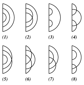
FIG. 5.: Representants of distinct graphs of third order without insertions.

Analogously, with two insertions the main graph has a cubic energy denominator, see for example the graph $(16)$ in Fig. 6. Using these rules, the graph $(11)$ in Fig. 4 leads to the energy correction

$$\Delta_{n}^{(2,11)} = g^{2}\int_{-\infty}^{\infty}d\epsilon_{1}\int_{-\infty}^{\infty}d\epsilon_{2}\frac{\epsilon_{1}e^{-|\epsilon_{1}|/D}}{1-e^{-\beta\epsilon_{1}}}\frac{\epsilon_{2}e^{-|\epsilon_{2}|/D}}{1-e^{-\beta\epsilon_{2}}}$$ (50)

$$\frac{1}{(\xi_{-1}+\epsilon_{1})^{2}}\frac{1}{\xi_{1}+\epsilon_{2}}$$

that factorizes into $(-1)$ times the graph $(2)$ in Fig. 3 with the energy denominator squared, multiplied with the graph $(1)$ in Fig. 3. These insertions are shorthand notations for graphs with decorations that stem from a pole of higher order in the energy denominator multiplied with a lower order graph. Therefore the higher order denominators and the factors $(-1)$ correspond to derivatives with respect to the auxiliary variable $E$. At zero temperature these graphs are related to terms in the Rayleigh-Schrödinger perturbative expansion stemming from normalization [28].

FIG. 6.: Representants of distinct graphs of third order with insertions.

In the high temperature limit, or equivalently in the limit $E_{C}\rightarrow 0$, the Wick theorem implies that only “connected” graphs appear in the exponent. The “connected” graphs are those where all processes occur in one channel. In order $g^{m}$, $m>1$, these “connected” graphs, however, give only $1/{\cal N}$ corrections that we have omitted. Hence, in the high temperature limit only the first order graphs survive and all higher order terms have to cancel. For the second order terms it turns out that each column in Fig. 4 cancels. For example, the contribution of the first column, graphs $(1),(5)$, and $(9)$, leads at vanishing charging energy to

$$\Delta_{n}^{(2;1,5,9)}\bigg{|}_{E_{C}\equiv 0}$$ (51)

$$= g^{2}\int_{-\infty}^{\infty}d\epsilon_{1}\int_{-\infty}^{\infty}d\epsilon_{2}\frac{\epsilon_{1}e^{-|\epsilon_{1}|/D}}{1-e^{-\beta\epsilon_{1}}}\frac{\epsilon_{2}e^{-|\epsilon_{2}|/D}}{1-e^{-\beta\epsilon_{2}}}$$ (53)

$$\times\left[\frac{1}{\epsilon_{1}^{2}(\epsilon_{1}+\epsilon_{2})}+\frac{1}{\epsilon_{1}(\epsilon_{1}+\epsilon_{2})\epsilon_{2}}-\frac{1}{\epsilon_{1}^{2}\epsilon_{2}}\right]$$

$$\equiv 0\,.$$ (54)

Higher order diagrams cancel likewise, and therefore in the limit of a large channel number the perturbative expansion can be truncated after the first term at high temperatures where the charging energy $E_{C}$ is negligible compared to the thermal energy $k_{B}T$.

The application of the diagrammatic rules to higher order graphs is obvious and we just present the contribution corresponding to graph $(7)$ in Fig. 5

$$\Delta_{n}^{(3,7)}$$ (55)

$$= \!\!-g^{3}\int_{-\infty}^{\infty}d\epsilon_{1}\int_{-\infty}^{\infty}d\epsilon_{2}\int_{-\infty}^{\infty}d\epsilon_{3}$$ (58)

$$\!\!\frac{\epsilon_{1}e^{-|\epsilon_{1}|/D}}{1-e^{-\beta\epsilon_{1}}}\frac{\epsilon_{2}e^{-|\epsilon_{2}|/D}}{1-e^{-\beta\epsilon_{2}}}\frac{\epsilon_{3}e^{-|\epsilon_{3}|/D}}{1-e^{-\beta\epsilon_{3}}}\big{[}(\xi_{1}+\epsilon_{1})(\xi_{2}+\epsilon_{1}+\epsilon_{2})$$

$$\!\!\times(\xi_{3}+\epsilon_{1}+\epsilon_{2}+\epsilon_{3})(\xi_{2}+\epsilon_{1}+\epsilon_{3})(\xi_{1}+\epsilon_{3})\big{]}^{-1}$$

as an example of a third order term. Here, three tunneling processes occur and we have to deal with five energy denominators. In this graph the excess charge number is raised three times and then lowered stepwise. The energy denominators include the quasiparticle excitation energies of arcs that would be intersected by a horizontal line. While the creation and annihilation times $\alpha_{j}$, $(j=1,\ldots,2m)$ of these quasiparticle excitations are already integrated out, the order of creation and annihilation of different excitations is crucial. All types of diagrams of third order PT without insertions are depicted in Fig. 5 and the graphs with one or two insertions are shown in Fig. 6. Here, we have omitted different combinations of semicircles to the left and right but displayed only one representant. Hence, each graph in Figs. 5 and 6 stands for $8$ different left-right combinations of the $3$ semicircles. Further, the diagrams $(7)$ and $(8)$ in Fig. 5 and $(11)$ and $(12)$ in Fig. 6 are topologically distinct from graphs reflected at a horizontal line, but obviously, they lead to identical contributions and we have to count them twice.

In summary, we have $80$ topologically different graphs without insertions, $64$ with one and $16$ graphs with two insertions leading to $160$ topologically different graphs of third order. All contributions of third order are readily evaluated using the rules given above. In general, there are always $2^{m}$ left-right combinations for one representant of order $m$. Moreover, the number of representants exceeds the $(2m-1)!!$ possibilities to arrange $m$ semicircles along the vertical line, simply as a consequence of the summation over insertions. Hence, the number of graphs of order $m$ exceeds $(2m)!/m!$, i.e. grows faster than the factorial. This rough estimation leads to more than $120$ graphs in third and more than $1680$ graphs in fourth order, showing that a reasonable treatment is limited to third order. To obtain higher order or nonperturbative results, one has to limit oneself to partial summations of graphs including the essential contributions. Unfortunately, in the infinite cutoff limit $D\rightarrow\infty$, each graph of the perturbative series represents a diverging integral and only the full sum in each order remains finite [24]. Hence, partial summations of higher order graphs need an artificial cutoff complicating a direct comparison with experimental findings. Consequently, within PT, the systematical treatment of higher orders is the only tool to get results directly comparable with experiments. To proceed we discuss two general simplifications, valid for all orders.

C Reflected Graphs

The analytical form of the integrals leads to general consequences for energy corrections. First we note that the particular form of the charging energy $(\ref{eq:coulomben})$ implies

$$E_{n}(n_{g})=E_{n+1}(n_{g}+1)=E_{-n}(-n_{g})$$ (59)

and the corresponding energy differences in the denominators read

$$\xi_{\pm p}=E_{n\pm p}(n_{g})-E_{n}(n_{g})=E_{C}[p^{2}\pm 2p(n-n_{g})]$$ (60)

which depends, on the difference $(n-n_{g})$ only.

FIG. 7.: Symmetry of two vertically reflected graphs.

Hence, the corrections of order $m$ may be written in the form

$$\Delta_{n}^{(m)}(n_{g})=g^{m}E_{C}f_{m}(n-n_{g}).$$ (61)

Since contributions of order $m$ include always $m$ integrals with $2m-1$ energy denominators, we gain by measuring all energies in units of $E_{C}$ a single factor $E_{C}$, and in the limit of an infinite bandwidth, $D\rightarrow\infty$, the functions $f_{m}$ depend on $\beta E_{C}$ only. Further, a reflection of a given graph on the vertical axis leads to the same contribution with the replacement $E_{n\pm p}\rightarrow E_{n\mp p}$, cf. Fig. 7. Equivalently, by virtue of Eq. $(\ref{eq:coulombid})$, one can replace $(n-n_{g})$ by $-(n-n_{g})$. Since the sum over diagrams includes all left-right permutations of arcs including pairs of vertically reflected graphs, one may write

$$f_{m}(u)=g_{m}(u)+g_{m}(-u),$$ (62)

where the contribution of $g_{m}$ solely includes topologically different graphs where one arc is held fixed.

D Insertions

A further simplification arises for graphs with insertions. It turns out that they factorize into a host graph, with energy denominator squared, and an insertion contribution. Since we have to sum over all possible left-right configurations, the full lower order contribution may be inserted. In Fig. 8 ${\rm a})$ we replace a first order insertion and its vertically reflected companion by a circle representing a multiplication with the full first order contribution $\Delta_{n}^{(1)}$. Likewise, insertions of order $k$ and all possible left-right combinations lead to a multiplication with the full order $k$ contribution $\Delta_{n}^{(k)}$, schematically depicted for $k=2$ by the square in Fig. 8 ${\rm b})$. The double arrow in this figure represents the sum over all possible left-right arrangements of semicircles belonging to the insertion. Therefore, all graphs belonging to the representants $(13),(14),$ and $(15)$ in Fig. 6 lead to

$$\Delta_{n}^{(3,13-15)} = -g^{3}E_{C}f_{2}(u)\int_{-\infty}^{\infty}d\epsilon\frac{\epsilon e^{-|\epsilon|/D}}{1-e^{-\beta\epsilon}}\frac{1}{(\xi_{1}+\epsilon)^{2}}$$ (64)

$$+(u\rightarrow-u),$$

with $u=n-n_{g}$. This is a multiplication of three factors, $\Delta_{n}^{(2)}$ and the host graph $(1)$ in Fig. 3 with the energy denominator squared, and $(-1)$. Additionally, we have added the contribution of the vertically reflected graphs which is of the same form with the replacement $u\rightarrow-u$. Likewise, all graphs belonging to the representant $(16)$ in Fig. 6 lead to

$$\Delta_{n}^{(3,16)} = -g^{3}E_{C}^{2}f_{1}(u)^{2}\int_{-\infty}^{\infty}d\epsilon\frac{\epsilon e^{-|\epsilon|/D}}{1-e^{-\beta\epsilon}}\frac{1}{(\xi_{1}+\epsilon)^{3}}$$ (66)

$$+(u\rightarrow-u)\,,$$

which is a multiplication of $\left(\Delta_{n}^{(1)}\right)^{2}$ and the host graph $(1)$ in Fig. 3 with the energy denominator cubed. This procedure holds for insertions of all order and is used in Sec. VI to resum the leading logarithmic divergencies in the two-state approximation.

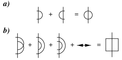
FIG. 8.: a) full first and b) full second order insertions.

IV Zero Temperature Limit and Third Order

In this section we perform the zero temperature limit and present results of third order.

A Zero Temperature Limit

Generally, at zero temperature the partition function of a system with nondegenerate discrete energy levels depends only on the ground state energy

$$Z=\sum_{n=-\infty}^{+\infty}e^{-\beta(E_{n}+\Delta_{n})}\longrightarrow e^{-\beta{\cal E}}.$$ (67)

Due to the restriction of the gate voltage to the range $0\leq n_{g}<\scriptstyle{\frac{1}{2}}$, the ground state charge number is $n=0$ and the ground state energy reads ${\cal E}=E_{0}+\Delta_{0}$. Therefore, the energy differences in the denominators read

$$\xi_{\pm p}=E_{\pm p}-E_{0}=E_{C}(p^{2}\mp 2pn_{g})$$ (68)

and the functions $f_{m}$ and $g_{m}$ depend on $n_{g}$ only. The average island charge number reduces to

$$\langle n\rangle=n_{g}-\frac{1}{2E_{c}}~{}\frac{\partial{\cal E}}{\partial n_{g}}\,.$$ (69)

Bose factors in the integrands restrict the integration $(\ref{eq:energintt})$ to positive energies

$$g\int_{-\infty}^{\infty}d\epsilon\frac{\epsilon e^{-|\epsilon|/D}}{1-e^{-\beta\epsilon}}\longrightarrow g\int_{0}^{\infty}d\epsilon\epsilon e^{-\epsilon/D}$$ (70)

which facilitates the integration, because there are no poles from the energy denominator $(\ref{eq:energydenom})$ that need to be taken care of, meaning there are no real excitations.

B First and Second Order Results

The first and second order calculations were already presented in Ref. [24]. The first order with an exponential cutoff $D$ leads to

$$g_{1}(u)=-(1+2u)\ln(1+2u)-D/E_{C}+\ln(D/E_{C})+\gamma,$$ (71)

where $\gamma=0.577\ldots$ is Euler’s constant. In the infinite cutoff limit this term diverges, but the derivative with respect to $n_{g}$ remains finite. When we restrict ourselves to first order in $g$, we may omit this divergence, however, in combination with higher order terms in the perturbative series, i.e. as lower order insertion, we have to use the full expression $(\ref{eq:firstorder})$. Whereas the first order contribution diverges, the full sum of graphs of each higher order $m>1$ remains finite [24]. The second order contribution was also calculated previously leading to

$$g_{2}(u)$$ (72)

$$= \frac{\pi^{2}}{6}(1+2u+8u^{2})-\left(\frac{5}{2}-4u+2u^{2}\right)\ln^{2}\left(\frac{1-2u}{4(1-u)}\right)$$ (76)

$$+\left(\frac{1}{4}+u+u^{2}\right)\ln^{2}\left(\frac{1-2u}{1+2u}\right)$$

$$+(1+2u)\ln\left(\frac{1-2u}{1+2u}\right)-4(1-u)\ln\left(\frac{1-2u}{4(1-u)}\right)$$

$$-(5-8u+4u^{2}){\rm Li}_{2}\left(\frac{3-2u}{4(1-u)}\right),$$

where ${\rm Li}_{2}(u)$ is the dilogarithm function [29].

C Third Order

Here, we motivate the calculation of the third order contribution exemplarily for the graph $(7)$ in Fig. 5. The full analytic expression $g_{3}(u)$ is presented in the Appendix.

Since the integral over the entire sum of $160$ integrands remains finite, we may omit the cutoff. However, to calculate the integral analytically we have to separate the whole expression into tractable parts. Each integral will be divergent and we introduce a sharp high energy cutoff $D$. After integration we expand the expressions with respect to $D/E_{C}\rightarrow\infty$. There are divergent terms in each expression but the sum of divergencies of all graphs has to vanish. This cancellation serves as a useful, nontrivial test of our calculation. We have to deal with eight different types of integrands without insertions depicted in Fig. 5 and six different types with insertions in Fig. 6 (the graphs $(13)$ to $(15)$ are merged to a single graph with the whole second order contribution inserted). We exemplarily proceed with graph $(7)$ in Fig. 5 leading to an integral of type

$$h_{7} = \int_{0}^{D}d\epsilon_{1}\int_{0}^{D}d\epsilon_{2}\int_{0}^{D}d\epsilon_{3}\epsilon_{1}\epsilon_{2}\epsilon_{3}$$ (79)

$$\big{[}(\kappa_{1}+\epsilon_{1})(\kappa_{2}+\epsilon_{1}+\epsilon_{2})(\kappa_{3}+\epsilon_{1}+\epsilon_{2}+\epsilon_{3})$$

$$\times(\kappa_{4}+\epsilon_{1}+\epsilon_{3})(\kappa_{5}+\epsilon_{3})\big{]}^{-1}\,.$$

where the $\kappa_{j}$ stand for excitation energies of the form $(\ref{eq:coulenergdiff})$. The full contribution of this representant consists of all possible left-right arrangements of the semicircles leading to

$$\Delta_{0}^{(3,7)}=-g^{3}\sum h_{7}(\kappa_{1},\kappa_{2},\kappa_{3},\kappa_{4},\kappa_{5}),$$ (80)

where the sum runs over all allowed combinations of energy differences. These are $h_{7}(\xi_{1},\!\xi_{2},\!\xi_{3},\!\xi_{2},\!\xi_{1})$, $h_{7}(\xi_{1},\!0,\!\xi_{1},\!\xi_{2},\!\xi_{1})$, $h_{7}(\xi_{1},\!0,\!\xi_{-1},\!0,\!\xi_{-1})$, $h_{7}(\xi_{1},\!\xi_{2},\!\xi_{1},\!0,\!\xi_{-1})$, and all terms with $n_{g}\rightarrow-n_{g}$. The integrals may be performed by splitting denominators into partial fractions. Using

$$\frac{1}{(a+\epsilon_{2})(b+\epsilon_{2})}=\frac{1}{(a-b)(b+\epsilon_{2})}-\frac{1}{(a-b)(a+\epsilon_{2})}$$ (81)

where $a=\kappa_{2}+\epsilon_{1}$ and $b=\kappa_{3}+\epsilon_{1}+\epsilon_{3}$, we are able to perform the $\epsilon_{2}$ integral leading to a logarithm function

$$\int_{0}^{D}d\epsilon_{2}\frac{-\epsilon_{2}}{a+\epsilon_{2}}=a\ln(a+D)-a\ln(a)-D.$$ (82)

The new denominator $1/(a-b)$ on the rhs of Eq. $(\ref{eq:parfrac})$ has an artificial pole at $\epsilon_{3}=\kappa_{2}-\kappa_{3}$. Since the integrand is analytic in the integration region, the sum of all pole contributions has to cancel in the threefold integral $(\ref{eq:graphdritteord})$. However, each pole contribution depends on the contour of integration and we have to specify the contour and use the same for all integrals. Next we consider the $\epsilon_{1}$ integration. In the numerator now appears the logarithm function from the previous integration, $\ln(\kappa_{2}+\epsilon_{1})$, that diverges for $\epsilon_{1}\rightarrow 0$ when $\kappa_{2}\equiv 0$ and we temporarily introduce a lower integration limit. With a decomposition of the form $(\ref{eq:parfrac})$, where $\epsilon_{2}$ is replaced by $\epsilon_{1}$ and the constants read $a=\kappa_{1}$ and $b=\kappa_{4}+\epsilon_{3}$, we split the remaining fractions in $(\ref{eq:graphdritteord})$ and perform the integral in terms of the dilogarithm function [29]

$${\rm Li}_{2}(z)=-\int_{0}^{z}dz^{\prime}\frac{\ln(1-z^{\prime})}{z^{\prime}}.$$ (83)

The third integration can then be performed using the trilogarithm function ${\rm Li}_{3}(z)$, where the general polylogarithm functions are defined by [29]

$${\rm Li}_{n}(z)=\int_{0}^{z}dz^{\prime}\frac{{\rm Li}_{n-1}(z^{\prime})}{z^{\prime}}.$$ (84)

All terms emerging can be expressed by trilogarithms, dilogarithms, logarithms, and rational functions of $n_{g}$. Here, the arguments of the transcendental functions are rational expressions of energy differences. Since each integration increases the “order” of transcendental functions at most by one, the transcendental terms are of the form ${\rm Li}_{k}\ln^{l}$ obeying $k+l\leq 3$. Here $\ln^{l}$ stands for a product of $l$ logarithms of possibly different arguments. The “order” thereby characterizes the transcendental function for large arguments: e.g. ${\rm Li}_{k}\sim\ln^{k}$ is of order $k$. We find in order $m$ of the perturbative series transcendental terms of the form $({\rm Li}_{m})^{k_{m}}\cdots({\rm Li}_{2})^{k_{2}}\ln^{k_{1}}$ where $\sum_{j=1}^{m}jk_{j}\leq m$. In principle, the integrals in PT lead in all orders to analytically known functions but there are practical restrictions, in particular, since the integrals cannot be evaluated straightforwardly by tools like Mathematica because one has to take care of the integration contours and pole contributions explicitly. In view of the length of the analytical result we present $g_{3}(u)$ in the Appendix.

The result is in terms of complicated analytical functions that have to be calculated numerically. Therefore, one could think of a direct numerical evaluation of the three fold integrals, but there are serious numerical problems. First, only the full sum of the $160$ integrals is finite and one has to use a huge integrand. Moreover, the integrand is not symmetric in the three integration variables, in particular, there are integration directions where the integrand leads to diverging positive and negative contributions. For a numerical study one has to symmetrize the integrand which enlarges it by a factor of $6$. Second, in spite of the smoothness and analyticity of the integrand and the absence of poles in the integration region, the integrand contains oscillatory parts so that standard numerical routines fail. We used a statistical integration routine to check the analytical predictions for selected parameter values. Typically, the numerical evaluation of a single point with a few per cent accuracy took over a week of CPU on a SGI Origin 200. Therefore, a numerical evaluation of the integral in third order is hopeless, in particular for delicate high precision studies regarding the limiting behavior near the degeneracy point or calculations of second order derivatives needed to determine the charging energy.

V Average Charge Number

The analytical result for the average island charge number $\langle n\rangle$ at zero temperature and in first order in $g$ was calculated previously [5, 30]

$$\langle n\rangle_{1}=g\ln\frac{1+2n_{g}}{1-2n_{g}}$$ (85)

and can be readily obtained by using Eq. $(\ref{eq:nmittel2})$ with the energy correction $(\ref{eq:firstorder})$. The function is well behaved except at the degeneracy point $n_{g}=\scriptstyle{\frac{1}{2}}$ where it exhibits a logarithmic divergence $\langle n\rangle_{1}\sim-g\ln\delta$, with $\delta={\scriptstyle\frac{1}{2}}-n_{g}$. Therefore, the range of validity of the perturbative series at zero temperature is strictly restricted to $n_{g}<\scriptstyle{\frac{1}{2}}$. The contribution of second order in $g$ presented in Ref. [31] reads

$$\langle n\rangle_{2}$$ (86)

$$= -g^{2}\Bigg{\{}n_{g}\left[\frac{4\pi^{2}}{3}+\ln^{2}\left(\frac{1-2n_{g}}{1+2n_{g}}\right)\right]$$ (90)

$$+\frac{16(1+2n_{g}-2n_{g}^{2})}{(3-2n_{g})(1+2n_{g})}\ln(1-2n_{g})$$

$$+2(1-n_{g})\Bigg{[}\ln^{2}\left(\frac{1-2n_{g}}{4(1-n_{g})}\right)+2\mbox{Li}_{2}\left(\frac{3-2n_{g}}{4(1-n_{g})}\right)$$

$$-\frac{8(1-n_{g})}{(1-2n_{g})(3-2n_{g})}\ln(4(1-n_{g}))\Bigg{]}-(n_{g}\rightarrow-n_{g})\Bigg{\}}\,.$$

Here, $(n_{g}\rightarrow-n_{g})$ stands for the same sum of terms with $n_{g}$ replaced by $-n_{g}$ showing explicitly the asymmetry of $\langle n\rangle$ with respect to the applied voltage $U_{g}$. At the degeneracy point, a leading logarithmic divergency of $\langle n\rangle_{2}\sim-2g^{2}\ln^{2}\delta$ appears. This indicates that near the degeneracy point $g\ln\delta$ is the effective expansion parameter so that the larger $g$ the smaller is the range of $n_{g}$ where finite order PT suffices. The analytical result of third order is not given explicitly here but can easily be calculated by differentiating the expression $\Delta_{0}^{(3)}$ with respect to $n_{g}$, cf. $(\ref{eq:nmittel2})$. Also the third order term shows a logarithmic divergency at the degeneracy point leading together with the lower order contributions to the asymptotic expansion

$$\langle n\rangle = ag^{2}+bg^{3}-(g+6g^{2}+cg^{3})\ln\delta$$ (92)

$$-(2g^{2}+24g^{3})\ln^{2}\delta-4g^{3}\ln^{3}\delta+{\cal O}\left(\delta,g^{4}\right)\,,$$

where the coefficients $a$ and $c$ read

$$a = 3-\frac{5}{3}\pi^{2}-\frac{9}{2}\ln(3)+3\ln^{2}(3)+6\,{\rm Li}_{2}\left(\frac{2}{3}\right)$$ (93)

$$= -9.7726\ldots\,,$$ (94)

$$c = 21+\frac{21}{4}\pi^{2}+9\ln(3)-6\ln^{2}(3)-12\,{\rm Li}_{2}\left(\frac{2}{3}\right)$$ (95)

$$= 65.462\ldots\,.$$ (96)

In view of its length the coefficient $b$ is given only numerically, $b=-70.546...$, but it can be readily obtained from the analytical result of $\Delta_{0}^{(3)}$ in the Appendix. The leading order logarithmic terms in Eq. (92) read

$$\langle n\rangle\sim-g\ln\delta-2g^{2}\ln^{2}\delta-4g^{3}\ln^{3}\delta\,.$$ (97)

They are related to diagrams that contain only the charge states $n=0$ and $1$. Therefore, before comparing our findings with numerical results, we consider a two-state approximation restricted to these degenerate charge states.

VI Degeneracy Point

FIG. 9.: Full ground state energy diagram in the non-crossing approximation of the two-state model.

A further analysis of the perturbative series in the limit of $n_{g}\rightarrow\scriptstyle{\frac{1}{2}}$ shows that the leading logarithmic divergencies $(\ref{eq:nmittel4})$ stem from diagrams including only charge states $n=0$ and $1$. This is a direct consequence of the degeneracy of these charge states at $n_{g}=\scriptstyle{\frac{1}{2}}$. The two-state approximation limits the perturbative series to graphs that contain the charge states $n=0,1$ only. This model was shown to be equivalent to an anisotropic multi channel Kondo Hamiltonian where $E_{C}\delta$ corresponds to the magnetic field and $g$ to the exchange integral [5]. Considering the leading order logarithmic divergencies we find that crossed diagrams, like graph $(6)$ in Fig. 5 with the middle semicircle to the left, do not contribute. Therefore, we may restrict ourselves to noncrossing diagrams. It is then possible to write the ground state energy as

$$\widetilde{\Delta}_{0}=g\int_{0}^{D}d\epsilon\epsilon F_{1}(\epsilon)$$ (98)

graphically represented in Fig. 9. The generalized energy denominator $F_{1}(\epsilon)$ corresponds to the bold line with index $1$ and is determined by a Dyson equation graphically represented in Fig. 10. For convenience, we have rotated the graphs by $90$ degrees and an upper (lower) semicircle increases (lowers) the charge number. Further, since we sum a subset of graphs, we need to introduce a cutoff $D$, which for convenience is chosen as a sharp cutoff.

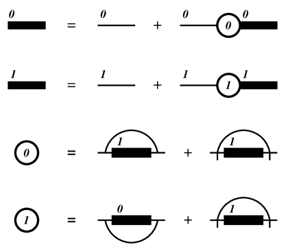
FIG. 10.: Dyson equation in the non-crossing approximation of the two-state model.

In the Dyson equation depicted in Fig. 10 the thin line with index $0$ corresponds to the bare energy denominator $-1/\epsilon$ of the charge state $0$ where $\epsilon$ is the energy variable. Analogously, the thin line with index $1$ correspond to the bare energy denominator $-1/(\xi_{1}+\epsilon)$ of charge state $1$. On the other hand, the bold line with index $0$ $(1)$ represents the dressed $n=0$ $(n=1)$ propagator $F_{0}(\epsilon)$ $(F_{1}(\epsilon))$ arising from the insertion of interaction vertices according to the first (second) line in Fig. 10. Hereby the interaction vertex represented by a circle with index $0$ $(1)$ is composed of a semicircle and an insertion according to the third (fourth) line in Fig. 10. These diagrams are evaluated by employing the rules given in Sec. III. Each part of an interaction vertex contains an integral $g\int_{0}^{D}d\epsilon^{\prime}\epsilon^{\prime}$ but the two pieces differ in the explicit meaning of $\epsilon^{\prime}$: While the insertion is just a multiplication where the propagator inside does not depend on the energy variable $\epsilon$ of the legs of the vertex, the semicircle propagator takes into account all excitation energies and therefore depends on $\epsilon+\epsilon^{\prime}$. Due to the restriction of the perturbative series to the charge states $n=0$ and $n=1$, the interaction vertices contain only two parts shown in Fig. 10, and the Dyson equation generates all diagrams in the non-crossing approximation. However, to be consistent with the truncation to two charge states, one has to introduce a cutoff $D$ that restricts electron-hole pair excitations to energies lower than the next charge state. With higher energy excitations being eliminated the parameters must be interpreted as effective renormalized quantities.

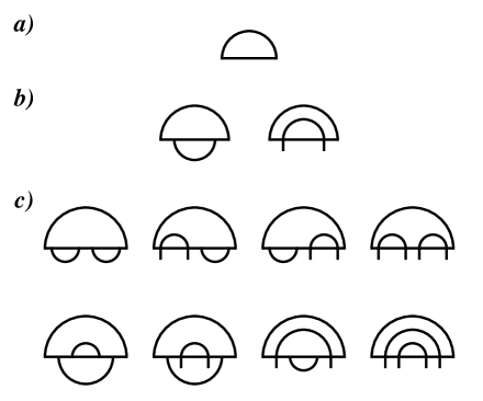
FIG. 11.: Graphs of a) first, b) second, and c) third order in the two-state model generated by the Dyson equation in Fig. 10.

One way to find the renormalization of the parameters is a comparison of the limiting divergent behavior for $n_{g}\rightarrow\scriptstyle{\frac{1}{2}}$ with the full PT result. This comparison leads to a series expansion of the renormalized parameters $g^{*}$ and $E_{C}^{*}$ in terms of the bare conductance $g$.

Iterating the Dyson equation we generate graphs including only charge states $n=0,1$. In Fig. 11 we depict all graphs of a) first, b) second, and c) third order in $g$ obtained this way. However, not all of these graphs contribute to the leading behavior near $n_{g}\rightarrow\scriptstyle{\frac{1}{2}}$. We find that only graphs of the form shown in Fig. 12 are responsible for the leading logarithmic divergencies in order $g^{m}$. The diagram ${\rm a})$ shows $m-1$ downward arcs leading to the asymptotic behavior

$$\widetilde{\Delta}_{0}^{(m,0)}\sim-g^{m}\delta\ln^{m}\delta$$ (99)

for $\delta\rightarrow 0$. The diagram ${\rm b})$ shows $m-k-1$ arcs lowering the charge state and one multi-insertion represented as an insertion with a slash with label $k$ $(k<m)$ which stands for the full result in the two-state approximation in order $k$. Assuming that the order $k$ result has the leading order behavior

$$\widetilde{\Delta}_{0}^{(k)}\sim-\frac{1}{2}\left(2g\ln\delta\right)^{k}\delta$$ (100)

as is apparent for $k=1,2$ and $3$ form Eq. $(\ref{eq:nmittel4})$, these graphs asymptotically behave as

$$\widetilde{\Delta}_{0}^{(m,k)}\sim\widetilde{\Delta}_{0}^{(k)}\,g^{m-k}\frac{\ln^{m-k}\delta}{m-k}=-g^{m}\,\frac{2^{k-1}}{m-k}\,\delta\ln^{m}\delta\,.$$ (101)

Interchange of the multi-insertion and the arcs leads to topologically different contributions that have to be counted separately. This leads to a factor $(m-k)$ canceling the denominator in Eq. $(\ref{eq:dysonkinsert})$. The sum over all $k$’s starting with $k=0$ as represented by graph ${\rm a})$ in Fig. 12 and from $k=1$ to $k=m-1$ corresponding to graph ${\rm b})$ leads to an asymptotic behavior of the form

$$\widetilde{\Delta}_{0}^{(m)}\sim\sum_{k=0}^{m-1}\widetilde{\Delta}_{0}^{(m,k)}=-\frac{1}{2}\left(2g\ln\delta\right)^{m}\delta$$ (102)

which proves the assumption $(\ref{eq:assumption})$ for all $k$ by induction. For the average island charge number $(\ref{eq:nmittel2})$ we obtain by summing over all orders in $g$

$$\langle n\rangle=\frac{-g\ln\delta}{1-2g\ln\delta}\,.$$ (103)

This result was originally obtained by Matveev [5] with RG techniques. While this result does not depend explicitly on the cutoff $D$, it contains renormalized parameters $g$ and $\delta$ depending on the tunneling strength. The leading logarithmic divergencies up to third order coincide with those given in Eq. $(\ref{eq:nmittel4})$, however, nonleading divergencies from Eq. $(\ref{eq:nmittel3})$ are missing. They can be included by using renormalized parameters $g^{*}$ and $\delta^{*}$ in Eq. $(\ref{eq:matveev})$. Since the energy difference between the two charge states is $E_{C}\delta$, the renormalization of the charging energy may be written as $E_{C}\delta^{*}$. The renormalized quantities are then found to read

$$g^{*}=g\left[1+6g+c_{2}g^{2}+{\cal O}(g^{3})\right]$$ (104)

and

$$\delta^{*}=\delta\left[1+d_{1}g+d_{2}g^{2}+{\cal O}(g^{3})\right]$$ (105)

where the renormalization factors are given as series in powers of $g$ with coefficients that may be expressed in terms of the expansion coefficients in Eqs. $(\ref{eq:nmittel3})$–$(\ref{eq:nmittel32})$. We have $c_{2}=-4a-c=-26.372\ldots$, $d_{1}=-a=9.7726\ldots$, and $d_{2}=6a+a^{2}/2-b=59.662\ldots$. As a consequence of the rapidly increasing series coefficients the result $(\ref{eq:matveev})$ with $(\ref{eq:grenormal})$ and $(\ref{eq:drenormal})$ does not lead to meaningful results in the vicinity of $n_{g}=\scriptstyle{\frac{1}{2}}$ except for very small $g$. Therefore, one has to resum also nonleading divergencies in the two-state approximation to describe the behavior near $n_{g}=\scriptstyle{\frac{1}{2}}$. This has not been considered so far but is the aim of future work.

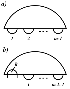
FIG. 12.: Diagrams of order $g^{m}$ contributing to the leading logarithmic divergencies.

VII Discussion of Results

In this section we compare our analytical results with numerical data and estimate the range of validity of various orders of PT. While various QMC studies of the single electron box are available [20, 21, 22, 25], only the data in Ref. [25] determine the island charge number for finite gate voltages and very low temperatures so that they can be compared with zero temperature predictions. Further, we confront our results with the findings of a recent renormalization group study [9]. The comparison of first, second, and third order PT with QMC data [25] and RG results [9] for $\alpha=2,5$, and $10$ is shown in Fig. 13. Not to overload the graph for $\alpha=2$ the RG results are omitted but they coincide with third order PT. We give results here in terms of the dimensionless tunneling conductance $\alpha=G_{T}/G_{K}=4\pi^{2}g$. We find good agreement for gate voltages near zero, but for $n_{g}\rightarrow\scriptstyle{\frac{1}{2}}$ the analytic result diverges. As discussed above the range of validity of PT shrinks with increasing gate voltage. We find that third order PT in $\alpha$ remains valid with errors below $4\%$ up to $n_{g}\approx 0.495$ for dimensionless conductance $\alpha=2$, up to $n_{g}\approx 0.45$ for $\alpha=5$, and up to $n_{g}\approx 0.4$ for $\alpha=10$. In these parameter intervals PT agrees both with QMC and RG data. Since for $n_{g}=0.45$ the charging energies for $n=0$ and $n=1$ differ only by $0.1E_{C}$, deviations from the third order result in $\alpha$ can be observed only for temperatures well below $E_{C}/10k_{B}$ even at $n_{g}={\scriptstyle\frac{1}{2}}$. Hence, at finite temperature the range of validity of PT increases. Further, Fig. 13 shows that the resummation of the leading logarithmic terms $(\ref{eq:matveev})$ does not suffice to describe the behavior near $n_{g}={\scriptstyle\frac{1}{2}}$. Subleading logarithms are important to obtain quantitatively meaningful results in the strong tunneling regime. We remark that the inclusion of subleading logarithmic terms of low orders only, in terms of the renormalized parameters $g^{*}$ and $\delta^{*}$ defined in Eqs. $(\ref{eq:grenormal})$ and $(\ref{eq:drenormal})$, does not improve the agreement, rather one has to consistently resum the nonleading logarithmic terms to all orders.

FIG. 13.: The average electron number $\langle n\rangle$ as a function of the dimensionless voltage $n_{g}$ is shown in first, second, and third order perturbation theory in $\alpha$, and compared with QMC data [25] and RG results [9]. The result $(\ref{eq:matveev})$ is also shown as a dotted line.

Since for $n_{g}\rightarrow 0$ the QMC and RG data perfectly coincide with the perturbative results, we used a more sensitive quantity to determine the range of validity of PT in this limit: For small external voltages, the average island charge grows linearly as

$$\langle Q\rangle=e\langle n\rangle=C^{*}U_{g}$$ (106)

where $C^{*}$ is an effective capacitance of the box. In the absence of Coulomb blockade effects $C^{*}=C$, while for strong Coulomb blockade, i.e., in the limit of vanishing tunneling conductance, $C^{*}=0$. It is thus natural to characterize the strength of the Coulomb blockade effect by an effective charging energy $E_{C}^{*}$ defined by [20]

$$\frac{E_{C}^{*}}{E_{C}}=1-\frac{C^{*}}{C}=1-\left.\frac{\partial\langle n\rangle}{\partial n_{g}}\right|_{n_{g}=0}.$$ (107)

One may view $E_{C}^{*}$ as the effective rounding of the energy parabolas at $n_{g}=0$ in the presence of tunneling. The perturbative series gives

$$\frac{E_{C}^{*}}{E_{C}}=1-4g+Ag^{2}-Bg^{3}+{\cal O}(g^{4}),$$ (108)

where

$$A = \frac{8\pi^{2}-32}{3}+\frac{64}{9}\ln(2)-16\ln^{2}(2)-8\,{\rm Li}_{2}\left(\frac{3}{4}\right)$$ (109)

$$= 5.066...$$ (110)

and $B=1.457...$ is given here only numerically in view of the length of the analytical expression.

FIG. 14.: Effective charging energy as a function of the dimensionless conduction $\alpha=G_{T}/G_{K}$. Perturbative findings are compared with QMC data [20, 21, 22, 25] and RG results [9].

In Fig. 14 we compare our predictions for the effective charging energy with QMC data by Wang, Egger, and Grabert [20] (WEG), Hofstetter and Zwerger [21] (HZ), Herrero, Schön, and Zaikin [22] (HSZ), and Göppert et al. [25] (GGPS) and RG results by König and Schoeller [9]. We find good agreement with PT up to $\alpha\approx 8$ for second order PT, while third order PT extends to $\alpha\approx 16$. Discrepancies between these QMC studies only arise outside of the range of validity of third order PT.

VIII Fluctuations of the average charge number

In this section we study the steady state fluctuations of the average charge number $\langle n\rangle$. We are mainly interested in the variance $\langle\delta n^{2}\rangle$ with $\delta n=n-\langle n\rangle$. Since $(n-n_{g})^{2}=\partial H_{C}/\partial E_{C}$, one may calculate this quantity in terms of a derivative of the free energy. At zero temperature, the free energy to first order PT is given by $E_{C}[g_{1}(n_{g})+g_{1}(-n_{g})]$ with the function $g_{1}$ defined in Eq. $(\ref{eq:firstorder})$. However, this result would lead to a logarithmic divergence of $\langle\delta n^{2}\rangle$ for large electronic bandwidth $D$. The same divergence occurs also at finite temperatures, cf. Ref. [24]. To explore where this cutoff dependence comes from, we consider the correlation function $\langle\delta n(t)\delta n(0)\rangle$. Using PT this quantity is well defined for finite $t$ but diverges in the limit $t\rightarrow 0$. This divergence is found to result from a $1/\omega$ tail for large $\omega$ in the fluctuation spectrum arising from the coupling to high energy electron-hole excitations. While this tail is cut off by the finite bandwidth $D$, in real experiments there is a cutoff from the time resolution of the measurement device at a certain frequency $\omega_{M}$ well below $D/\hbar$. To avoid these cutoff effects, we discuss only the noise spectrum

$$S_{n}(\omega)=\int dte^{i\omega t}C(t)$$ (111)

that is the Fourier transform of the symmetrized correlation function

$$C(t)=\frac{1}{2}\langle\delta n(t)\delta n(0)+\delta n(0)\delta n(t)\rangle\equiv\langle\delta n(t)\delta n(0)\rangle^{s}\,.$$ (112)

While $S_{n}(\omega)$ also depends on the electronic bandwidth, for frequencies well below the electronic cutoff and not too low temperatures the spectrum becomes independent of the bandwidth. Here, $\delta n(t)=\exp(i{\rm L}t)n-\langle n\rangle$ is the fluctuation of the average charge number in the Heisenberg representation, where the time evolution is governed by the Liouville operator ${\rm L}X=\frac{1}{\hbar}[H,X]$.

Since a direct perturbative expansion of $C(t)$ results effectively in a short time expansion, it is insufficient to determine the low frequency behavior of $S_{n}(\omega)$ properly. Here, we use projection operator techniques [32] to derive a formally exact integral equation for the dynamics of $C(t)$ and then expand the kernel in powers of the dimensionless conductance $g$. The adequate projector reads

$$PX=\frac{\delta n}{\langle\delta n^{2}\rangle}\langle\delta nX\rangle^{s}$$ (113)

which fulfills the requirement $P^{2}=P$. Applying the time evolution operator one finds the relation

$$Pe^{i{\rm L}t}P=\bar{C}(t)P\,,$$ (114)

with the normalized correlator $\bar{C}(t)=C(t)/\langle\delta n^{2}\rangle$. Further, the time derivative of the correlator may be written in the form

$$\dot{\bar{C}}(t)P=Pe^{i{\rm L}t}i{\rm L}P.$$ (115)

Using the operator identity

$$Pe^{i{\rm L}t}=Pe^{i{\rm L}t}P+\int_{0}^{t}dsPe^{i{\rm L}s}Pi{\rm L}\bar{P}e^{i\bar{P}{\rm L}\bar{P}(t-s)}\,,$$ (116)

with $\bar{P}=1-P$, Eq. $(\ref{eq:correlderiv})$ may be written as

$$\dot{\bar{C}}(t)P = Pe^{i{\rm L}t}Pi{\rm L}P$$ (118)

$$+\int_{0}^{t}dsPe^{i{\rm L}s}Pi{\rm L}\bar{P}e^{i\bar{P}{\rm L}\bar{P}(t-s)}i{\rm L}P\,.$$

Inserting the identity $(\ref{eq:projcid})$ we get the exact evolution equation

$$\dot{C}(t)=\frac{\langle\delta n\dot{n}\rangle^{s}}{\langle\delta n^{2}\rangle}C(t)-\int_{0}^{t}ds\phi(t-s)C(s)\,,$$ (119)

with the memory kernel

$$\phi(t)=\frac{\langle\dot{n}\dot{n}_{r}(t)\rangle^{s}}{\langle\delta n^{2}\rangle}-\frac{\langle\delta n\dot{n}\rangle^{s}}{\langle\delta n^{2}\rangle}\frac{\langle\delta n\dot{n}_{r}(t)\rangle^{s}}{\langle\delta n^{2}\rangle}\,.$$ (120)

Here, the reduced time evolution of $\dot{n}$ is given by

$$\dot{n}_{r}(t)=e^{i\bar{P}{\rm L}\bar{P}t}\dot{n}\,.$$ (121)

The linear equation $(\ref{eq:cintegeq})$ can be solved by means of a Laplace transformation yielding

$$\widehat{C}(z)=\frac{C(0)}{z-\langle\delta n\dot{n}\rangle^{s}/\langle\delta n^{2}\rangle+\widehat{\phi}(z)}$$ (122)

which is related to the noise spectrum by

$$S_{n}(\omega)\! = \!\int_{-\infty}^{\infty}dte^{i\omega t}C(t)=2{\rm Re}\int_{0}^{\infty}dte^{i\omega t}C(t)$$ (123)

$$= \!2{\rm Re}\!\lim_{z\rightarrow-i\omega}\!\int_{0}^{\infty}\!\!\!dte^{-zt}C(t)\!=\!2{\rm Re}\lim_{z\rightarrow-i\omega}\widehat{C}(z)\,.$$ (124)

To evaluate the right hand side of Eq. $(\ref{eq:noiselapl})$ we first determine the initial value $C(0)=\langle n^{2}\rangle-\langle n\rangle^{2}$ in second order in the tunneling Hamiltonian by means of a straightforward expansion of the density matrix using the imaginary time methods in Sec. III A. Since $n$ and $n^{2}$ are diagonal in charge representation, both averages may be written in the form

$$\!\!\!\!\!\!\langle X\rangle=\frac{1}{Z}{\rm tr}\left\{e^{-\beta H}X\right\}$$ (125)

$$= \frac{1}{Z}{\rm tr}\Big{\{}e^{-\beta H_{0}}\Big{[}1-\int_{0}^{\beta}\!\!d\tau^{\prime}H_{T}(\tau^{\prime})+$$ (127)

$$\quad\int_{0}^{\beta}d\tau^{\prime}\int_{0}^{\tau^{\prime}}\!\!d\tau^{\prime\prime}H_{T}(\tau^{\prime})H_{T}(\tau^{\prime\prime})\Big{]}X\Big{\}}$$

$$= \frac{Z_{0}}{Z}\Big{\langle}X+\!\sum_{\zeta=\pm}\int_{0}^{\beta}\!\!\!d\tau^{\prime}\int_{0}^{\tau^{\prime}}\!\!\!d\tau^{\prime\prime}Y(\tau^{\prime}-\tau^{\prime\prime})e^{-(\tau^{\prime}-\tau^{\prime\prime})\xi_{\zeta}}X\Big{\rangle}_{C}\,,$$ (128)

with the free partition function $Z_{0}={\rm tr}\exp(-\beta H_{0})$ and the Coulomb energy differences $\xi_{\zeta}$ that were introduced in Eq. $(\ref{eq:coulenergdiff})$. Here, we have decomposed the trace into a Coulomb and a quasiparticle trace as in Sec. III A, and have introduced the free Coulomb average

$$\langle X\rangle_{C}=\sum_{n=-\infty}^{\infty}e^{-\beta E_{n}}X\Bigg{/}\sum_{n=-\infty}^{\infty}e^{-\beta E_{n}}\,.$$ (129)

Inserting the representation $(\ref{eq:greensf})$ for the electron-hole pair propagator into Eq. $(\ref{eq:imagexp})$, the time integrals are readily evaluated leading to an energy integral that may be solved by contour integration, cf. Ref. [24]. For the average charge number squared we find

$$\langle n^{2}\rangle = \langle n^{2}\rangle_{C}(1+\langle K_{1}\rangle_{C})$$ (131)

$$-\langle n^{2}K_{1}+2nK_{2}+K_{3}\rangle_{C}+{\cal O}(g^{2})\,.$$

The first term $\langle K_{1}\rangle_{C}$ stems from the expansion of the denominator $Z$ where

$$K_{1}=2\pi g{\rm Im}\sum_{\zeta=\pm}[f_{1}(iE_{C}/\nu)-f_{1}(i\xi_{\zeta}/\nu)]$$ (132)

and $\nu=2\pi/\beta$. A divergent part for $D\rightarrow\infty$ is omitted since it is canceled by a corresponding term in the expansion of the numerator. Further, we introduced the auxiliary function

$$f_{1}(x)=x\psi(1+x)$$ (133)

where $\psi(z)$ is the logarithmic derivative of the gamma function. The remaining terms contain

$$K_{2}=g\sum_{\zeta=\pm}\zeta{\rm Re}[f_{1}^{\prime}(i\xi_{\zeta}/\nu)]$$ (134)

and

$$K_{3}=g\left\{2[\gamma-\ln(D/\nu)]+\sum_{\zeta=\pm}{\rm Re}[f_{1}^{\prime}(i\xi_{\zeta}/\nu)]\right\}\,.$$ (135)

Whereas $K_{1}$ and $K_{2}$ are independent of the cutoff, the last function diverges in the infinite bandwidth limit. For the average charge number we get likewise

$$\langle n\rangle=\langle n\rangle_{C}(1+\langle K_{1}\rangle_{C})-\langle nK_{1}+K_{2}\rangle_{C}\,.$$ (136)

Next, we determine $\langle\delta n\dot{n}\rangle^{s}$ where the time derivative of the charge number

$$\dot{n}=\frac{i}{\hbar}[H,n]=\frac{i}{\hbar}\sum_{kq\sigma}\left(t_{kq\sigma}a^{\dagger}_{k\sigma}a_{q\sigma}\Lambda-{\rm H.c.}\right)$$ (137)

arises from the tunneling Hamiltonian. Since $\dot{n}$ is of first order in the tunneling Hamiltonian and is off-diagonal in charge representation, we have to expand the density matrix up to first order, cf. Eq. $(\ref{eq:imagexp})$, and one readily finds $\langle\delta n\dot{n}\rangle^{s}={\cal O}(g^{2})$. Now, the only term contributing in second order in the tunneling Hamiltonian reads

$$\langle\dot{n}\dot{n}_{r}(t)\rangle^{s} = \frac{1}{Z_{0}}{\rm Re}\left[{\rm tr}\left\{e^{-\beta H_{0}}\dot{n}e^{\frac{i}{\hbar}H_{0}t}\dot{n}e^{-\frac{i}{\hbar}H_{0}t}\right\}\right]$$ (138)

$$= g{\rm Re}\left\langle\sum_{\zeta=\pm}\int d\epsilon\frac{\epsilon e^{-|\epsilon|/D}}{1-e^{-\beta\epsilon}}e^{-\frac{i}{\hbar}(\epsilon+\xi_{\zeta})t}\right\rangle_{C}\,,$$ (139)

where we have used that $\exp(i\bar{P}L_{0}\bar{P}t)\dot{n}=\exp(\frac{i}{\hbar}H_{0}t)\dot{n}\exp(-\frac{i}{\hbar}H_{0}t)+{\cal O}(g)$. The Laplace transform can be readily performed leading to

$$\!\widehat{\phi}(z)\! = \frac{g}{2\langle\delta n^{2}\rangle_{C}}\sum_{\zeta,\zeta^{\prime}=\pm}\Bigg{\langle}\frac{\pi}{\hbar}\frac{-\xi_{\zeta}+i\zeta^{\prime}\hbar z}{1-e^{\beta(\xi_{\zeta}-i\zeta^{\prime}\hbar z)}}e^{-|\xi_{\zeta}+i\zeta^{\prime}\hbar z|/D}$$ (141)

$$+z\!\sum_{m=1}^{\infty}\!\frac{me^{-|\nu_{m}|/D}}{[m\!-(i\zeta^{\prime}\xi_{\zeta}-\hbar z)/\nu][m-(i\zeta^{\prime}\xi_{\zeta}+\hbar z)/\nu]}\!\Bigg{\rangle}_{C}$$

which depends on the electronic bandwidth $D$ and shows a $1/z$ dependence for $z\gg D/\hbar$. The spectral density of the charge fluctuations now follows from Eqs. $(\ref{eq:noiselapl})$ and $(\ref{eq:noiselaplfour})$. Since the measurement device suppresses frequencies above a cutoff $\omega_{M}\ll D/\hbar$, we may focus on $|z|\ll D/\hbar$ and find

$$\widehat{\phi}(z) = \frac{g}{2\langle\delta n^{2}\rangle_{C}}\sum_{\zeta,\zeta^{\prime}=\pm}\Bigg{\langle}\frac{\pi}{\hbar}\frac{-\xi_{\zeta}+i\zeta^{\prime}\hbar z}{1-e^{\beta(\xi_{\zeta}-i\zeta^{\prime}\hbar z)}}$$ (144)

$$\quad-\zeta^{\prime}\frac{\nu}{2\hbar}\sum_{\kappa=\pm}f_{1}\left(\frac{i\kappa\xi_{\zeta}+\zeta^{\prime}\hbar z}{\nu}\right)\Bigg{\rangle}_{C}$$

$$\quad+2gz\frac{\ln(D/\nu)-\gamma}{\langle\delta n^{2}\rangle_{C}}$$

which determines the noise spectrum for frequencies $|\omega|\ll D/\hbar$:

$$S_{n}(\omega)=2\mbox{Re}\frac{C(0)}{-i\omega+\widehat{\phi}(-i\omega)}\,.$$ (145)

While $\widehat{\phi}(z)$ has been evaluated to first order in $g$ the spectrum $S_{n}(\omega)$ contains terms of all orders in $g$.

Two approximations can be considered:

i) For large $|\omega|\gg\exp(-\langle\delta n^{2}\rangle_{C}/g)D/\hbar$ we may expand the denominator in Eq. $(\ref{eq:noisespec})$

$$\frac{C(0)}{-i\omega+\widehat{\phi}(-i\omega)}=C(0)\left[\frac{1}{-i\omega}+\frac{\widehat{\phi}(-i\omega)}{\omega^{2}}+{\cal O}(g^{2})\right]$$ (146)

and get the perturbative result which reads for $|\omega|\ll D/\hbar$

$$S_{n}(\omega) = 2\pi C^{f}(0)\delta(\omega)$$ (148)

$$+g\frac{\pi}{\hbar\omega^{2}}\sum_{\zeta\zeta^{\prime}=\pm}\left\langle\frac{\zeta^{\prime}\hbar\omega-\xi_{\zeta}}{1-e^{-\beta(\zeta^{\prime}\hbar\omega-\xi_{\zeta})}}\right\rangle_{C}+{\cal O}(g^{2})\,,$$

in accordance with earlier findings [33]. Here, the diverging parts of $C(0)$ in Eq. $(\ref{eq:K3withco})$ and of $\widehat{\phi}(-i\omega)$ in Eq. $(\ref{eq:kernel1zllD})$ cancel leading to the finite contribution $C^{f}(0)=C(0)+\langle K_{3}\rangle_{C}$ independent of the cutoff $D$. However, this approximation is not valid at small frequencies and shows a $1/\omega^{2}$ divergence that cannot describe the low frequency behavior correctly. In contrast, for large frequencies the result $(\ref{eq:noisepert})$ is well behaved and merges with our result $(\ref{eq:noisespec})$.

ii) On the other hand, for small $z\ll\pi k_{B}T/\gamma\hbar$ at large temperatures $k_{B}T\gg E_{C}$ and/or $z\ll\pi E_{C}\exp(-\beta E_{C})/\hbar\ln(\beta E_{C})$ at moderate to low temperatures $k_{B}T{{\lower 2.0pt\hbox{$<$}\atop\raise 5.0pt\hbox{$\sim$}}}E_{C}$ we may replace $\widehat{\phi}(z)$ by $\widehat{\phi}(0)+\widehat{\phi}^{\prime}(0)z$ which is often referred to as Markovian approximation. Then

$$\widehat{C}(z)=\frac{C(0)}{z[1+\widehat{\phi}^{\prime}(0)]+\widehat{\phi}(0)}$$ (149)

where $\widehat{\phi}^{\prime}(0)=-\langle K_{3}\rangle_{C}/\langle\delta n^{2}\rangle_{C}$. In the limit $2g\ln(D/\nu)\ll\langle\delta n^{2}\rangle_{C}$ we may expand $1+\phi^{\prime}(0)$ around $g=0$ and get

$$S_{n}(\omega)=C^{f}(0)\frac{2\widehat{\phi}(0)}{\omega^{2}+\widehat{\phi}(0)^{2}}\,.$$ (150)

While the Markovian approximation fails to describe the high frequency behavior, at high temperatures the classical result

$$\widetilde{C}_{M}(\omega)=\frac{k_{B}TC}{e^{2}}\frac{2G_{T}/C}{\omega^{2}+(G_{T}/C)^{2}}$$ (151)

is recovered. Hence, at high temperatures the first order approximation $(\ref{eq:kernel1zllD})$ of the memory kernel $\phi(t)$ becomes exact.

Now, provided the experimental cutoff $\omega_{M}$ is small enough for the Markovian approximation to be justified we have

$$\langle\delta n(t)\delta n(0)\rangle_{M}^{s}=\frac{1}{2\pi}\int d\omega S_{n}(\omega)F(\omega/\omega_{M})e^{-i\omega t}$$ (152)

with a cutoff function $F(\omega/\omega_{M})$ obeying $F(0)=1$. Using contour integration we get in the limit $t\rightarrow 0$

$$\langle\delta n^{2}\rangle_{M}=C^{f}(0)F(\widehat{\phi}(0)/\omega_{M})=C^{f}(0)+{\cal O}(\widehat{\phi}(0)/\omega_{M})\,.$$ (153)

Hence, for $\widehat{\phi}(0)\ll\omega_{M}\ll D/\hbar$ the measured variance is independent of the cutoff.

To show the impact of finite tunneling conductance we compare in Fig. 15 the variance $(\ref{eq:varianceMarkov})$ of the average charge number in the Markovian approximation for $\alpha=0$ (thin lines) and $\alpha=1$ (bold lines) for different temperatures in dependence on the dimensionless gate voltage $n_{g}$. Whereas tunneling amplifies the noise near $n_{g}=0$, in the vicinity of the degeneracy point the noise is suppressed by tunneling leading to the asymptotic behavior $\langle\delta n^{2}\rangle_{M}\approx{\scriptstyle\frac{1}{4}}-g[\ln(\beta E_{C}/\pi)+1+\gamma]$. Since fluctuations of the charge are related to the linear conductance of the single electron transistor (SET) this behavior is in accordance with the observation that the linear conductance of the SET increases with the tunneling strength off the degeneracy point and on the other hand decreases directly at the degeneracy point, cf. Refs. [18, 34, 35].

FIG. 15.: Variance of the average charge number in dependence on the dimensionless gate voltage for different temperatures. Depicted are the results for $\alpha=0$ (thin lines) compared with results for $\alpha=1$ (bold lines).

Finally, we remark that directly at the degeneracy point $\widehat{\phi}(z)$ becomes nonanalytic at zero temperatures for $z\rightarrow 0$ and the Markovian approximation breaks down. Therefore, at lower temperatures $k_{B}T\ll E_{C}$ one has to use the full bandwidth dependent expression $(\ref{eq:kernelD})$.

IX Conclusions

In this article charge fluctuations of the single electron box were investigated by means of perturbation theory. Terms of third order in the phenomenological tunneling conductance were calculated analytically in the zero temperature limit. The predictions for the average charge number and the effective charging energy have been compared with Monte-Carlo data and renormalization group results. It has been shown that the perturbative treatment, in spite of its diverging behavior at the degeneracy point, leads to reliable results in a large part of the parameter regime explored experimentally. An additional order in the perturbative series increases the range of validity considerably, in particular for small gate voltages $n_{g}\approx 0$ where PT covers the largest range of conductance parameters $\alpha$. When increasing the gate voltage the range shrinks continuously down to zero at the degeneracy point $n_{g}={\scriptstyle\frac{1}{2}}$. In the vicinity of the degeneracy point we have evaluated all graphs contributing to the leading logarithmic divergencies. A resummation was found to be insufficient to describe the behavior of the average charge number in the strong tunneling regime quantitatively. It turns out that nonleading logarithmic divergencies are essential, the summation of which remains an open problem.

Further, the noise spectrum of the average charge number has been investigated. In contrast to the average charge number this quantity depends on the electronic bandwidth $D$. Using a projection operator technique we have obtained an expression covering the perturbative as well as the semiclassical results. We find that in the Coulomb blockade region near $n_{g}=0$ strong tunneling leads to an increase of the noise whereas at the degeneracy point $n_{g}={\scriptstyle\frac{1}{2}}$ the noise is suppressed.

Third Order Result

In this appendix we give the explicit analytic result of the contribution in the third order in $g$ to the ground state energy ${\cal E}$. According to the transcendental functions appearing in the various terms we split the result into six contributions

$$g_{3}(u)=P3(u)+P2(u)+L3(u)+L2(u)+L1(u)+R(u)\,.$$ (154)

Here $P3$ contains all terms with trilogarithms ${\rm Li}_{3}$ while $P2$ lists those with dilogarithms ${\rm Li}_{2}$. Terms containing logarithms and no other transcendental functions are split into three types: In $L3$ and $L2$ expressions containing $\ln^{3}$ and $\ln^{2}$ are listed, respectively. Simple logarithms appear in $L1$ and the remaining rational functions of $u$ and constants are gathered in $R$. With the abbreviation

$$\xi_{n}^{m}=\xi_{m}-\xi_{n}$$ (155)

these terms read

$$\!\!\!\!\!\!\!\!\!\!P3(u)=$$ (156)

$$\!\!\!\!\!\!\!\!\!\!\left({\frac{207}{4}}+{\frac{223\,u}{2}}+105\,{u^{2}}+34\,{u^{3}}\ \right)\,{\rm Li}_{3}\left({\frac{\xi_{1}}{\xi_{2}}}\right)+\left({\frac{79}{2}}+{\frac{211\,u}{2}}+102\,{u^{2}}+34\,{u^{3}}\ \right)\,{\rm Li}_{3}\left({\frac{\xi_{1}^{2}}{\xi_{2}}}\right)$$ (157)

$$\!\!\!\!\!\!\!\!\!\!+\xi_{1}\,\left[{\rm Li}_{3}\left({\frac{\xi_{-1}^{2}}{2\,\xi_{2}}}\right)-2\,{\rm Li}_{3}\left({\frac{\xi_{1}}{2\,\xi_{1}^{2}}}\right)+{\rm Li}_{3}\left({\frac{\xi_{1}}{2\,{\xi_{1}^{3}}}}\right)+{\rm Li}_{3}\left({\frac{\xi_{2}^{3}}{2\,\xi_{2}}}\right)-2\,{\rm Li}_{3}\left({\frac{\xi_{2}^{3}}{2\,\xi_{1}^{2}}}\right)+{\rm Li}_{3}\left({\frac{3\,\xi_{2}^{3}}{2\,{\xi_{1}^{3}}}}\right)\right]$$ (158)

$$\!\!\!\!\!\!\!\!\!\!-\left({\frac{63}{4}}+{\frac{31\,u}{2}}+9\,{u^{2}}+2\,{u^{3}}\right)\,{\rm Li}_{3}\left({\frac{\xi_{1}}{\xi_{3}}}\right)-\left({\frac{127}{8}}+{\frac{55\,u}{4}}+{\frac{9\,{u^{2}}}{2}}+{u^{3}}\right)\,\left[{\rm Li}_{3}\left({\frac{\xi_{1}^{2}\,\xi_{3}}{\xi_{2}\,\xi_{1}^{3}}}\right)\right.$$ (159)

$$\!\!\!\!\!\!\!\!\!\!+\left.{\rm Li}_{3}\left({\frac{\xi_{1}\,\xi_{2}^{3}}{\xi_{2}\,\xi_{1}^{3}}}\right)\right]+\left({\frac{7}{8}}+{\frac{15\,u}{4}}+{\frac{9\,{u^{2}}}{2}}+{u^{3}}\right)\,\left[{\frac{1}{2}{\rm Li}_{3}\left({\frac{(\xi_{-1}^{-2}+\xi_{2})\,\xi_{3}}{{{({\xi_{1}^{3}})}^{2}}}}\right)}-{\rm Li}_{3}\left({\frac{\xi_{-1}^{-2}+\xi_{2}}{{\xi_{1}^{3}}}}\right)\right.$$ (160)

$$\!\!\!\!\!\!\!\!\!\!+\left.{\rm Li}_{3}\left({\frac{\xi_{1}}{{\xi_{1}^{3}}}}\right)-2\,{\rm Li}_{3}\left({\frac{{\xi_{1}^{3}}}{\xi_{3}}}\right)\ \right]-\left({\frac{5}{2}}-{\frac{3\,u}{2}}-6\,{u^{2}}-2\,{u^{3}}\right)\,{\rm Li}_{3}\left({\frac{\xi_{-1}}{\xi_{2}^{3}}}\right)+\left({\frac{15}{4}}-6\,u-3\,{u^{2}}\right)\,$$ (161)

$$\!\!\!\!\!\!\!\!\!\!\times{\rm Li}_{3}\left({\frac{\xi_{2}}{\xi_{2}^{3}}}\right)-\left(18+8\,u\right)\,{\rm Li}_{3}\left({\frac{\xi_{2}^{3}}{\xi_{3}}}\right)+\left({\frac{119}{8}}+{\frac{47\,u}{4}}+{\frac{9\,{u^{2}}}{2}}+{u^{3}}\right)\,\left[{\rm Li}_{3}\left({\frac{\xi_{1}^{2}}{{\xi_{1}^{3}}}}\right)+{\rm Li}_{3}\left({\frac{\xi_{2}^{3}}{{\xi_{1}^{3}}}}\right)\right]$$ (162)

$$\!\!\!\!\!\!\!\!\!\!+\left({\frac{25}{16}}-{\frac{15\,u}{8}}-{\frac{9\,{u^{2}}}{4}}-{\frac{{u^{3}}}{2}}\right)\,{\rm Li}_{3}\left({\frac{\xi_{1}^{-2}\,\xi_{1}^{2}}{{{(\xi_{2}^{3})}^{2}}}}\right)\,.$$ (163)

$$\!\!\!\!\!\!\!\!\!\!P2(u)=$$ (164)

$$\!\!\!\!\!\!\!\!\!\!4\left(1+4\,{u^{2}}\right)\ln\left({\frac{\xi_{-1}}{\xi_{1}}}\right)\left[{\rm Li}_{2}\left({\frac{\xi_{1}}{2}}\right)-{\rm Li}_{2}\left({\frac{-\xi_{-1}}{\xi_{1}}}\right)\right]-\left({\frac{33}{2}}+59\,u+62\,{u^{2}}+20\,{u^{3}}\right)\,\ln\left({\frac{\xi_{1}}{\xi_{1}^{2}}}\right)$$ (165)

$$\!\!\!\!\!\!\!\!\!\!\times{\rm Li}_{2}\left({\frac{2\,\xi_{2}}{{{(\xi_{1}^{2})}^{2}}}}\right)+\!\left(33+118\,u+124\,{u^{2}}+40\,{u^{3}}\right)\ln\left({\frac{\xi_{1}}{\xi_{1}^{2}}}\right){\rm Li}_{2}\left({\frac{2}{\xi_{1}^{2}}}\right)\!\!-\!\!\left({\frac{127}{8}}+{\frac{55\,u}{4}}+{\frac{9\,{u^{2}}}{2}}+{u^{3}}\right)$$ (166)

$$\!\!\!\!\!\!\!\!\!\!\times\ln\left({\frac{\xi_{1}\,\xi_{2}^{3}}{\xi_{1}^{2}\,\xi_{3}}}\right){\rm Li}_{2}\left({\frac{\xi_{1}^{2}\,\xi_{3}}{\xi_{2}\,\xi_{1}^{3}}}\right)+\left({\frac{119}{8}}+{\frac{47\,u}{4}}+{\frac{9\,{u^{2}}}{2}}+{u^{3}}\right)\,\ln\left({\frac{\xi_{1}^{2}}{\xi_{2}^{3}}}\right)\,{\rm Li}_{2}\left({\frac{\xi_{2}^{3}}{\xi_{1}^{3}}}\right)-\Bigg{[}49+72\,u+36\,{u^{2}}$$ (167)

$$\!\!\!\!\!\!\!\!\!\!+\left({\frac{49}{4}}+6\,u+3\,{u^{2}}\right)\,\ln(\xi_{2})+\left({\frac{37}{8}}+{\frac{39\,u}{4}}+{\frac{3\,{u^{2}}}{2}}+{u^{3}}\right)\,\ln(\xi_{-1})+\Bigg{(}{\frac{145}{8}}+{\frac{425\,u}{4}}+{\frac{239\,{u^{2}}}{2}}$$ (168)

$$\!\!\!\!\!\!\!\!\!\!+39\,{u^{3}}\Bigg{)}\,\ln(\xi_{1})-\left({\frac{145}{8}}+{\frac{425\,u}{4}}+{\frac{239\,{u^{2}}}{2}}+39\,{u^{3}}\right)\,\ln(\xi_{1}^{2})-\Bigg{(}{\frac{135}{8}}+{\frac{63\,u}{4}}+{\frac{9\,{u^{2}}}{2}}+{u^{3}}\Bigg{)}\,\ln(\xi_{2}^{3})\Bigg{]}\,$$ (169)

$$\!\!\!\!\!\!\!\!\!\!\times{\rm Li}_{2}\left({\frac{\xi_{1}^{2}}{\xi_{2}}}\right)+\left({\frac{7}{16}}+{\frac{15\,u}{8}}+{\frac{9\,{u^{2}}}{4}}+{\frac{{u^{3}}}{2}}\right)\,\ln\left({\frac{{{(\xi_{1})}^{2}}}{\left(\xi_{-1}^{-2}+\xi_{2}\right)\,\xi_{3}}}\right)\,{\rm Li}_{2}\left({\frac{\left(\xi_{-1}^{-2}+\xi_{2}\right)\,\xi_{3}}{{{(\xi_{1}^{3})}^{2}}}}\right)$$ (170)

$$\!\!\!\!\!\!\!\!\!\!+\xi_{1}\,\ln\left({\frac{\xi_{-1}^{2}}{\xi_{2}^{3}}}\right)\,{\rm Li}_{2}\left({\frac{\xi_{2}^{3}}{2\,\xi_{2}}}\right)-\left({\frac{7}{8}}+{\frac{15\,u}{4}}+{\frac{9\,{u^{2}}}{2}}+{u^{3}}\right)\,\ln\left({\frac{\xi_{1}}{\xi_{-1}^{-2}+\xi_{2}}}\right)\,{\rm Li}_{2}\left({\frac{\xi_{-1}^{-2}+\xi_{2}}{\xi_{1}^{3}}}\right)$$ (171)

$$\!\!\!\!\!\!\!\!\!\!+\frac{1}{8}\bigg{\{}\left(25-30\,u-36\,{u^{2}}-8\,{u^{3}}\right)\,\ln 3-8\,\left({\frac{15}{4}}-6\,u-3\,{u^{2}}\right)\,\ln(\xi_{2})+\xi_{-1}\,\xi_{2}^{3}\,\big{[}\xi_{-1}\,\ln(\xi_{-1})$$ (172)

$$\!\!\!\!\!\!\!\!\!\!+\xi_{2}^{3}\,\ln(\xi_{1}^{2})\big{]}\bigg{\}}\,{\rm Li}_{2}\left({\frac{\xi_{2}}{\xi_{2}^{3}}}\right)-\bigg{\{}\frac{1}{2}\xi_{-1}^{-3}\xi_{1}-(11+6\,u)\,\ln 3-\frac{1}{\xi_{1}^{2}}\,\left[\xi_{-1}^{-3}\,\xi_{-2}^{-3}+\left({\xi_{-1}^{-2}}\right)^{2}\,\ln 3\right]$$ (173)

$$\!\!\!\!\!\!\!\!\!\!-\left({\frac{105}{8}}+{\frac{17\,u}{4}}-{\frac{9\,{u^{2}}}{2}}-{u^{3}}\right)\,\ln(\xi_{1})+\left({\frac{7}{8}}+{\frac{15\,u}{4}}+{\frac{9\,{u^{2}}}{2}}+{u^{3}}\right)\,\ln(\xi_{-1}^{-2}+\xi_{2})$$ (174)

$$\!\!\!\!\!\!\!\!\!\!+\left({\frac{247}{8}}+{\frac{95\,u}{4}}+{\frac{9\,{u^{2}}}{2}}+{u^{3}}\right)\,\ln(\xi_{1}^{2})-\left({\frac{135}{8}}+{\frac{63\,u}{4}}+{\frac{9\,{u^{2}}}{2}}+{u^{3}}\right)\,\ln(\xi_{2}^{3})\bigg{\}}\,{\rm Li}_{2}\left({\frac{\xi_{1}^{3}}{3\,\xi_{1}^{2}}}\right)$$ (175)

$$\!\!\!\!\!\!\!\!\!\!+\xi_{1}\,\ln\left({\frac{\xi_{1}}{3\,\xi_{2}^{3}}}\right)\,{\rm Li}_{2}\left({\frac{3\,\xi_{2}^{3}}{2\,\xi_{1}^{3}}}\right)-\bigg{\{}\left({\frac{95}{8}}+{\frac{39\,u}{4}}+{\frac{9\,{u^{2}}}{2}}+{u^{3}}\right)\,\ln 3+\frac{1}{\xi_{1}^{2}}\left[\xi_{-2}\,\xi_{-1}+\left(\xi_{-1}^{-2}\right)^{2}\,\ln 3\right]$$ (176)

$$\!\!\!\!\!\!\!\!\!\!-\frac{1}{2}\xi_{-2}\left(\xi_{1}^{2}+\xi_{-2}\right)-\left({\frac{135}{8}}+{\frac{63\,u}{4}}+{\frac{9\,{u^{2}}}{2}}+{u^{3}}\right)\,\ln(\xi_{1})+\left({\frac{127}{4}}+{\frac{55\,u}{2}}+9\,{u^{2}}+2\,{u^{3}}\right)\,\ln(\xi_{1}^{2})$$ (177)

$$\!\!\!\!\!\!\!\!\!\!-\left({\frac{119}{8}}+{\frac{47\,u}{4}}+{\frac{9\,{u^{2}}}{2}}+{u^{3}}\right)\,\ln(\xi_{2}^{3})\bigg{\}}\,{\rm Li}_{2}\left({\frac{\xi_{2}^{3}}{\xi_{3}}}\right)-\left[2\,\xi_{1}\,\ln(\xi_{1})-2\,\xi_{1}\,\ln(\xi_{2}^{3})\right]\,{\rm Li}_{2}\left({\frac{\xi_{2}^{3}}{2\,\xi_{1}^{2}}}\right)\,.$$ (178)

$$\!\!\!\!\!\!\!\!\!\!L3(u)=$$ (179)

$$\!\!\!\!\!\!\!\!\!\!{\frac{1}{16}\left(129+98\,u-164\,{u^{2}}+56\,{u^{3}}\right)\,\ln(\xi_{1})\,{{\ln(\xi_{2})}^{2}}}-{\frac{1}{8}\left(131-282\,u+276\,{u^{2}}-88\,{u^{3}}\right)\,{{\ln(\xi_{2})}^{3}}}$$ (180)

$$\!\!\!\!\!\!\!\!\!\!+{\frac{1}{16}\left(295-798\,u+804\,{u^{2}}-264\,{u^{3}}\right)\,{{\ln(\xi_{1})}^{2}}\,\ln(\xi_{1}^{2})}+\frac{1}{16}\left(559-1742\,u+1796\,{u^{2}}-584\,{u^{3}}\right)$$ (181)

$$\!\!\!\!\!\!\!\!\!\!\times{{\ln(\xi_{2})}^{2}}\,\ln(\xi_{1}^{2})-\left({\frac{49}{2}}-65\,u+62\,{u^{2}}-20\,{u^{3}}\right)\,\ln(\xi_{1})\,{{\ln(\xi_{1}^{2})}^{2}}-\left(33-118\,u+124\,{u^{2}}-40\,{u^{3}}\right)$$ (182)

$$\!\!\!\!\!\!\!\!\!\!\times\ln(\xi_{2})\,{{\ln(\xi_{1}^{2})}^{2}}-{\frac{1}{8}{{(\xi_{1})}^{2}}\,(\xi_{-1}^{-2}+\xi_{2})\,{{\ln(\xi_{1})}^{2}}\,\ln(\xi_{1}^{3})}+\frac{1}{48}\left(1087-3054\,u+3012\,{u^{2}}-968\,{u^{3}}\right)$$ (183)

$$\!\!\!\!\!\!\!\!\!\!\times{{\ln(\xi_{1}^{2})}^{3}}-{\frac{1}{16}\left(89-142\,u+60\,{u^{2}}-8\,{u^{3}}\right)\,{{\ln(\xi_{2})}^{2}}\,\ln(\xi_{2}^{3})}+\frac{1}{8}\left(119-94\,u+36\,{u^{2}}-8\,{u^{3}}\right)$$ (184)

$$\!\!\!\!\!\!\!\!\!\!\times\left[\ln(\xi_{1}^{2})\,{{\ln(\xi_{1}^{3})}^{2}}+\ln(\xi_{1})\,\ln(\xi_{2})\,\ln(\xi_{2}^{3})+\ln(\xi_{1})\,\ln(\xi_{1}^{3})\,\ln(\xi_{2}^{3})-2\,\ln(\xi_{1})\,\ln(\xi_{1}^{2})\,\ln(\xi_{2}^{3})\right]$$ (185)

$$\!\!\!\!\!\!\!\!\!\!+\left({\frac{183}{4}}-{\frac{71\,u}{2}}+9\,{u^{2}}-2\,{u^{3}}\right)\,\ln(\xi_{1})\,\ln(\xi_{1}^{2})\,\ln(\xi_{1}^{3})-\frac{1}{8}\left(105-34\,u-36\,{u^{2}}+8\,{u^{3}}\right)\ln(\xi_{1})\,{{\ln(\xi_{1}^{3})}^{2}}$$ (186)

$$\!\!\!\!\!\!\!\!\!\!-{\frac{1}{8}{{(\xi_{2}^{3})}^{2}}\,\xi_{-1}\,\ln(\xi_{2})\,\ln(\xi_{1}^{2})\,\ln(\xi_{2}^{3})}-{\frac{1}{12}{{(\xi_{1})}^{2}}\,(\xi_{-1}^{-2}+\xi_{2})\,{{\ln(\xi_{1}^{3})}^{3}}}+\frac{1}{8}\left(127-110\,u+36\,{u^{2}}-8\,{u^{3}}\right)$$ (187)

$$\!\!\!\!\!\!\!\!\!\!\times\left[{{\ln(\xi_{2})}^{2}}\,\ln(\xi_{1}^{3})+\ln(\xi_{2})\,{{\ln(\xi_{1}^{3})}^{2}}-2\,\ln(\xi_{1})\,\ln(\xi_{2})\,\ln(\xi_{1}^{3})-{{\ln(\xi_{1}^{3})}^{2}}\,\ln(\xi_{2}^{3})+\ln(\xi_{2}\,\xi_{1}^{3})\,{{\ln(\xi_{2}^{3})}^{2}}\right]$$ (188)

$$\!\!\!\!\!\!\!\!\!\!+{\frac{1}{8}\left(135-126\,u+36\,{u^{2}}-8\,{u^{3}}\right)\,\ln(\xi_{1}^{2})\,\ln(\xi_{1}^{3})\,\ln(\xi_{2}^{3})}-\frac{1}{16}\left(433-530\,u+252\,{u^{2}}-56\,{u^{3}}\right)$$ (189)

$$\!\!\!\!\!\!\!\!\!\!\times\ln(\xi_{1}^{2})\,{{\ln(\xi_{2}^{3})}^{2}}-{\frac{1}{24}\left(55+78\,u-60\,{u^{2}}+8\,{u^{3}}\right)\,{{\ln(\xi_{2}^{3})}^{3}}}+\frac{1}{8}\left(293-266\,u+108\,{u^{2}}-24\,{u^{3}}\right)$$ (190)

$$\!\!\!\!\!\!\!\!\!\!\times{{\ln(\xi_{1}^{2})}^{2}}\,\ln(\xi_{2}^{3})-{\frac{1}{16}\left(69-18\,u+140\,{u^{2}}+264\,{u^{3}}\right)\,{{\ln(\xi_{1})}^{2}}\,\ln(\xi_{-1})}+\left({\frac{37}{8}}-{\frac{39\,u}{4}}+{\frac{3\,{u^{2}}}{2}}-{u^{3}}\right)$$ (191)

$$\!\!\!\!\!\!\!\!\!\!\times\ln(\xi_{1})\,\ln(\xi_{2})\,\ln(\xi_{-1})-{\frac{1}{3}\left(10+48\,u+24\,{u^{2}}+32\,{u^{3}}\right)\,{{\ln(\xi_{-1})}^{3}}}+{\frac{1}{8}{{(\xi_{1})}^{2}}\,\xi_{-2}^{-3}\,{{\ln(\xi_{1})}^{2}}\,\ln(\xi_{-2})}$$ (192)

$$\!\!\!\!\!\!\!\!\!\!-{\frac{1}{16}\left(67+30\,u-12\,{u^{2}}+8\,{u^{3}}\right)\,\ln(\xi_{1})\,{{\ln(\xi_{-2})}^{2}}}-{\frac{1}{8}{{(\xi_{1})}^{2}}\,(\xi_{-1}^{-2}+\xi_{2})\,\ln(\xi_{1})\,\ln(\xi_{1}^{3})\,\ln(\xi_{-1}^{-2}+\xi_{2})}$$ (193)

$$\!\!\!\!\!\!\!\!\!\!-\frac{1}{8}\left(373-314\,u+108\,{u^{2}}-24\,{u^{3}}\right){{\ln(\xi_{1}^{2})}^{2}}\,\ln(\xi_{1}^{3})+{\frac{1}{8}{{(\xi_{1})}^{2}}\,(\xi_{-1}^{-2}+\xi_{2})\,\ln(\xi_{1}^{2})\,\ln(\xi_{1}^{3})\,\ln(\xi_{-1}^{-2}+\xi_{2})}$$ (194)

$$\!\!\!\!\!\!\!\!\!\!-{\frac{1}{8}\left(31+146\,u-188\,{u^{2}}+56\,{u^{3}}\right)\ln(\xi_{1})\,\ln(\xi_{2})\,\ln(\xi_{1}^{2})}+\frac{1}{16}\left(35-66\,u-12\,{u^{2}}+8\,{u^{3}}\right)\ln(\xi_{1})$$ (195)

$$\!\!\!\!\!\!\!\!\!\ \times{{\ln(\xi_{-2}^{-3})}^{2}}\!+\!{\frac{1}{8}\xi_{1}\,{{(\xi_{-2}^{-3})}^{2}}\ln(\xi_{1})\ln(\xi_{-2})\ln(\xi_{-1}^{-2})}\!+\!{\frac{1}{16}{{(\xi_{1})}^{2}}(\xi_{-1}^{-2}+\xi_{2})\left[{{\ln(\xi_{1})}^{2}}\!-\!{{\ln(\xi_{1}^{2})}^{2}}\right]\ln(\xi_{-1}^{-2}+\xi_{2})}$$ (196)

$$\!\!\!\!\!\!\!\!\!\!-\!{\frac{1}{8}\xi_{1}\,{{(\xi_{-2}^{-3})}^{2}}\,\ln(\xi_{1})\ln(\xi_{-1}^{-2})\ln(\xi_{-2}^{-3})}\!-\!{\frac{1}{8}{{(\xi_{1})}^{2}}\xi_{-2}^{-3}\ln(\xi_{1})\ln(\xi_{-2})\ln(\xi_{-2}^{-3})}\!-\!{\frac{1}{16}{{(\xi_{1})}^{2}}\,\xi_{-2}^{-3}{{\ln(\xi_{1})}^{2}}\ln(\xi_{-2}^{-3})}\,.$$ (197)

$$\!\!\!\!\!\!\!\!\!\!L2(u)=$$ (198)

$$\!\!\!\!\!\!\!\!\!\!\frac{-1}{\xi_{1}^{2}\,\xi_{-1}}\,\left[49+12\,\ln 2-u\,\left(38-16\,\ln 2\right)-4\,{u^{2}}\,\left(45-8\,\ln 2\right)+8\,{u^{3}}\,\left(15+8\,\ln 2\right)-64\,{u^{4}}\,\ln 2\right]$$ (199)

$$\!\!\!\!\!\!\!\!\!\!\times{{\ln(\xi_{1})}^{2}}+\big{[}49+2\,\ln 2-2\,\ln 3+4\,u\,\left(-18-\ln 2+\ln 3\right)+36\,{u^{2}}\big{]}\,\ln(\xi_{1})\,\ln(\xi_{2})$$ (200)

$$\!\!\!\!\!\!\!\!\!\!-\frac{1}{2\xi_{1}^{2}\,\xi_{1}}\,\big{[}127+6\,\ln 2-6\,\ln 3-4\,u\,\left(123+7\,\ln 2-7\,\ln 3\right)+8\,{u^{2}}\,(92+5\,\ln 2-5\,\ln 3)$$ (201)

$$\!\!\!\!\!\!\!\!\!\!-16\,{u^{3}}\,\left(33\ln 2-\ln 3\right)+144\,{u^{4}}\big{]}{{\ln(\xi_{2})}^{2}}+{\frac{2}{\xi_{1}^{2}}\,\left[-19+35\,u-20\,{u^{2}}+4\,{u^{3}}\right]\ln(\xi_{2})\,\ln(\xi_{1}^{2})}$$ (202)

$$\!\!\!\!\!\!\!\!\!\!-\frac{2}{\xi_{1}^{2}}\,\left[14+6\,\ln 2+18\,\ln 3-u\,\left(23+16\,\ln 2+18\,\ln 3\right)+4\,{u^{2}}\,\left(4+2\,\ln 2+\ln 3\right)-4\,{u^{3}}\right]$$ (203)

$$\!\!\!\!\!\!\!\!\!\!\times\ln(\xi_{1})\,\ln(\xi_{1}^{2})-\xi_{1}\,\ln 2\,{{\ln(\xi_{1}^{3})}^{2}}+\frac{1}{16}\big{[}176+32\,\ln 2+263\,\ln 3-2\,u\,\left(96+32\,\ln 2+79\,\ln 3\right)$$ (204)

$$\!\!\!\!\!\!\!\!\!\!+4\,{u^{2}}\,\left(16+9\,\ln 3\right)-8\,{u^{3}}\,\ln 3\big{]}\,{{\ln(\xi_{1}^{2})}^{2}}+\frac{1}{8}\big{[}16\,\ln 2+231\,\ln 3-2\,u\,(16\,\ln 2+79\,\ln 3)$$ (205)

$$\!\!\!\!\!\!\!\!\!\!+36\,{u^{2}}\,\ln 3-8\,{u^{3}}\,\ln 3\ \big{]}\,\ln(\xi_{1})\,\ln(\xi_{1}^{3})-\frac{1}{8}\big{[}119-94\,u+36\,{u^{2}}-8\,{u^{3}}\big{]}\,\ln 3\,\ln(\xi_{1})\,\ln(\xi_{2}^{3})$$ (206)

$$\!\!\!\!\!\!\!\!\!\!-\frac{1}{8}\big{[}373-314\,u+108\,{u^{2}}-24\,{u^{3}}\big{]}\,\ln 3\,\ln(\xi_{1}^{2})\,\ln(\xi_{1}^{3})+\frac{1}{8}\big{[}213-218\,u+108\,{u^{2}}-24\,{u^{3}}\big{]}\,\ln 3\,$$ (207)

$$\!\!\!\!\!\!\!\!\!\!\times\ln(\xi_{1}^{2})\ln(\xi_{2}^{3})-{\frac{1}{8}{{(\xi_{2}^{3})}^{2}}\,\xi_{-1}\,\ln 3\ln(\xi_{2})\ln(\xi_{2}^{3})}+\frac{1}{8}(135-126\,u+36\,{u^{2}}-8\,{u^{3}})\ln 3\ln(\xi_{1}^{3})\ln(\xi_{2}^{3})$$ (208)

$$\!\!\!\!\!\!\!\!\!\!-\frac{1}{16}(179-310\,u+180\,{u^{2}}-40\,{u^{3}})\,\ln 3\,{{\ln(\xi_{2}^{3})}^{2}}-\frac{1}{2}\big{[}13-8\,\ln 2-39\,u\,\ln 2+{u^{2}}\,\left(36-32\,\ln 2\right)$$ (209)

$$\!\!\!\!\!\!\!\!\!\!-4\,{u^{3}}\,\ln 2\big{]}\,\ln(\xi_{1})\,\ln(\xi_{-1})+\frac{1}{8\,\xi_{-1}}\,\big{[}48+25\,\ln 3+4\,u\,\left(12+5\,\ln 3\right)+32\,{u^{2}}\,\left(2-3\,\ln 3\right)$$ (210)

$$\!\!\!\!\!\!\!\!\!\!+16\,{u^{3}}\,\left(4-5\,\ln 3\right)-16\,{u^{4}}\,\ln 3\big{]}\ln(\xi_{1})\,\ln(\xi_{-2})-{\frac{1}{8}{{(\xi_{1})}^{2}}\,(\xi_{-1}^{-2}+\xi_{2})\,\ln 3\,\ln\left({\frac{\xi_{1}^{2}}{\xi_{1}^{3}}}\right)\,\ln(\xi_{-1}^{-2}+\xi_{2})}$$ (211)

$$\!\!\!\!\!\!\!\!\!\!-{\frac{1}{8}\xi_{1}\,{{(\xi_{-2}^{-3})}^{2}}\,\ln 3\,\ln(\xi_{1})\,\ln(\xi_{-2}^{-3})}\,.$$ (212)

$$\!\!\!\!\!\!\!\!\!\!L1(u)=$$ (213)

$$\!\!\!\!\!\!\!\!\!\!\left[6\,\xi_{2}+\left(295-798\,u+804\,u^{2}-264\,u^{3}\right)\,\frac{{\pi}^{2}}{48}-\xi_{1}\,{\ln\left(\frac{3}{2}\right)}^{2}-\left(19-16\,u+4\,u^{2}\right)\,\ln 3\,\frac{\xi_{2}}{2\,\xi_{1}^{2}}\right]\ln(\xi_{2})$$ (214)

$$\!\!\!\!\!\!\!\!\!\!-\bigg{[}\left(79-402\,u+356\,u^{2}-376\,u^{3}\right)\,\frac{{\pi}^{2}}{48}+\left(7-8\,u+4\,u^{2}\right)\,\ln 3\,\frac{\xi_{1}^{3}\,}{2\,\xi_{1}^{2}}+2\,\left(3-u\right)\,{\ln(3)}^{2}$$ (215)

$$\!\!\!\!\!\!\!\!\!\!+\xi_{1}\,\left(15+2\,\ln 2\,\ln 3\right)\bigg{]}\ln(\xi_{1})-\bigg{[}3\,\xi_{1}^{2}+\left(861-1354\,u+1100\,u^{2}-344\,u^{3}\right)\,\frac{{\pi}^{2}}{96}-2\,\xi_{1}\,{\ln(2)}^{2}$$ (216)

$$\!\!\!\!\!\!\!\!\!\!+\frac{1}{48}\bigg{[}\left(197+22\,u+12\,u^{2}-24\,u^{3}\right)\,{\pi}^{2}+6\,\left(47-62\,u+36\,u^{2}-8\,u^{3}\right)\,{\ln(3)}^{2}\bigg{]}\,\ln(\xi_{2}^{3})$$ (217)

$$\!\!\!\!\!\!\!\!\!\!-\bigg{[}\xi_{1}\,{\ln(2)}^{2}-{(\xi_{1})}^{2}\,(\xi_{-1}^{-2}+\xi_{2})\frac{{\pi}^{2}}{24}+\left(\frac{119}{8}-\frac{47\,u}{4}+\frac{9\,u^{2}}{2}-u^{3}\right)\,{\ln(3)}^{2}\bigg{]}\,\ln(\xi_{1}^{3})$$ (218)

$$\!\!\!\!\!\!\!\!\!\!-2\,\left(11-12\,u+4\,u^{2}\right)\,\ln 3-\frac{1}{16}\left(263-158\,u+36\,u^{2}-8\,u^{3}\right)\,{\ln(3)}^{2}\bigg{]}\,\ln(\xi_{1}^{2})$$ (219)

$$\!\!\!\!\!\!\!\!\!\!+{\frac{1}{96}{{(\xi_{1})}^{2}}\,(\xi_{-1}^{-2}+\xi_{2})\,\left[{{\pi}^{2}}-6\,{{\ln(3)}^{2}}\right]\,\ln(\xi_{-1}^{-2}+\xi_{2})}\,.$$ (220)

$$\!\!\!\!\!\!\!\!\!\!R(u)=$$ (221)

$$\!\!\!\!\!\!\!\!\!\!-{\frac{{{\pi}^{2}}}{2}}+6\,{{\pi}^{2}}\,\ln 2-48\,{{\ln(2)}^{3}}-\left[9-{\frac{265\,{{\pi}^{2}}}{96}}-{{\ln(2)}^{2}}\right]\,\ln 3+\left(11+37\,\ln 2\right)\,{{\ln(3)}^{2}}-\frac{953}{48}\,{\ln(3)}^{3}$$ (222)

$$\!\!\!\!\!\!\!\!\!\!-38\,\ln 3\,{\rm Li}_{2}\left({\frac{2}{3}}\right)-18\,\ln 3\,{\rm Li}_{2}\left({\frac{3}{4}}\right)+18\,{\rm Li}_{3}\left({\frac{1}{4}}\right)+38\,{\rm Li}_{3}\left({\frac{1}{3}}\right)+18\,{\rm Li}_{3}\left({\frac{3}{4}}\right)-{\frac{1845}{16}}\,\zeta(3)$$ (223)

$$\!\!\!\!\!\!\!\!\!\!+{u^{2}}\,\left[{\frac{4\,{{\pi}^{2}}}{3}}-{\frac{3\,{{\pi}^{2}}}{8}}\,\ln 3+4\,{{\ln(3)}^{2}}+{\frac{3}{4}}\,{{\ln(3)}^{3}}-{\frac{651}{4}}\,\zeta(3)\ \right]\,.$$ (224)

REFERENCES

- [1] Single Charge Tunneling, Vol. 294 of NATO ASI Series B, edited by H. Grabert and M. H. Devoret (Plenum, New York, 1992).
- [2] D. V. Averin and K. K. Likharev, in Mesoscopic Phenomena in Solids, Vol. 30 of Modern Problems in Condensed Matter Science, edited by B. L. Altshuler, P. A. Lee, and R. A. Webb (North-Holland, Amsterdam, 1991), p. 173.
- [3] G. L. Ingold and Y. V. Nazarov, in Ref. [1], p. 21.
- [4] D. V. Averin and Y. V. Nazarov, in Ref. [1], p. 217.
- [5] K. A. Matveev, Sov. Phys. JETP 72, 892 (1991).
- [6] H. Schoeller and G. Schön, Phys. Rev. B 50, 18436 (1994).
- [7] D. S. Golubev and A. D. Zaikin, Phys. Rev. B 50, 8736 (1994).
- [8] G. Falci, G. Schön, and G. T. Zimanyi, Phys. Rev. Lett. 74, 3257 (1995).
- [9] J. König and H. Schoeller, Phys. Rev. Lett. 81, 3511 (1998).
- [10] G. Schön and A. D. Zaikin, Phys. Rep. 198, 237 (1990).
- [11] G. Göppert and H. Grabert, Eur. Phys. J. B 16, 687 (2000).
- [12] E. Ben-Jacob, E. Mottola, and G. Schön, Phys. Rev. Lett. 51, 2064 (1983).
- [13] S. V. Panyukov and A. D. Zaikin, Phys. Rev. Lett. 67, 3168 (1991).
- [14] D. S. Golubev and A. D. Zaikin, Phys. Rev. B 46, 10903 (1992).
- [15] D. S. Golubev and A. D. Zaikin, JETP Lett. 63, 1007 (1996).
- [16] X. Wang and H. Grabert, Phys. Rev. B 53, 12621 (1996).
- [17] G. Göppert, X. Wang, and H. Grabert, Phys. Rev. B 55, R10213 (1997).
- [18] G. Göppert and H. Grabert, Phys. Rev. B 58, R10155 (1998).
- [19] G. Göppert and H. Grabert, C. R. Acad. Sci. 327, 885 (1999).
- [20] X. Wang, R. Egger, and H. Grabert, Europhys. Lett. 38, 545 (1997).
- [21] W. Hofstetter and W. Zwerger, Phys. Rev. Lett. 78, 3737 (1997).
- [22] C. P. Herrero, G. Schön, and A. D. Zaikin, Phys. Rev. B 59, 5728 (1999).
- [23] G. Göppert, B. Hüpper, and H. Grabert, Physica B 284-288, 1792 (2000).
- [24] H. Grabert, Phys. Rev. B 50, 17364 (1994).
- [25] G. Göppert, H. Grabert, N. V. Prokof’ev, and B. V. Svistunov, Phys. Rev. Lett. 81, 2324 (1998).
- [26] J. König, H. Schoeller, and G. Schön, Phys. Rev. B 58, 7882 (1998).
- [27] P. Lafarge et al., Z. Phys. B 85, 327 (1991).
- [28] G. Göppert, H. Grabert, and C. Beck, Europhys. Lett. 45, 249 (1999).
- [29] L. Lewin, Polylogarithms and Associated Functions (North Holland, New York, 1981).
- [30] D. Esteve, in Ref. [1], p. 109.
- [31] H. Grabert, Physica B 194-196, 1011 (1994).
- [32] H. Grabert, Projection Operator Techniques in Nonequilibrium Statistical Mechanics (Springer, New York, 1982).
- [33] G. Schön, Phys. Rev. B 32, 4469 (1985).
- [34] P. Joyez et al., Phys. Rev. Lett. 79, 1349 (1997).
- [35] J. König, H. Schoeller, and G. Schön, Phys. Rev. Lett. 78, 4482 (1997).