Phase Transitions and Oscillations in a Lattice Prey-Predator Model

Abstract

A coarse grained description of a two-dimensional prey-predator system is given in terms of a 3-state lattice model containing two control parameters: the spreading rates of preys and predators. The properties of the model are investigated by dynamical mean-field approximations and extensive numerical simulations. It is shown that the stationary state phase diagram is divided into two phases: a pure prey phase and a coexistence phase of preys and predators in which temporal and spatial oscillations can be present. The different type of phase transitions occuring at the boundary of the prey absorbing phase, as well as the crossover phenomena occuring between the oscillatory and non-oscillatory domains of the coexistence phase are studied. The importance of finite size effects are discussed and scaling relations between different quantities are established. Finally, physical arguments, based on the spatial structure of the model, are given to explain the underlying mechanism leading to oscillations.

I Introduction

The dynamics of interacting species has attracted a lot of attention since the pioneering works of Lotka [1] and Volterra [2]. In their independent studies, they showed that simple prey-predator models may exhibit limit cycles during which the populations of both species have periodic oscillations in time. However, this behavior depends strongly on the initial state, and it is not robust to the addition of more general non-linearities or to the presence of more than two interacting species [3]. In many cases the system reaches a simple steady-state.

A better understanding of the properties of such oscillations is clearly desirable, as such population cycles are often observed in ecological systems and the underlying causes remain a long-standing open question [4]. One of the best documented example concerns the Canadian lynx population. This population was monitored for more than hundred years (starting in 1820) from different regions of Canada. It was observed that the population oscillates with a period of approximately 10 years and that this synchronization was spatially extended over areas of several millions of square kilometers [5]. Several attempts were made to explain these facts (climatic effects, relations with the food-web, influence if the solar cycle) without success. More recently, Blasius et al. [4] introduced a deterministic three level vertical food-chain model. The three coupled nonlinear differential equations defining the model contain eight free parameters and two unknown nonlinear functions. The authors showed that an ad-hoc choice of the free parameters and nonlinear functions explains the experimental data for the Canadian lynx.

In such mean-field type models, it is assumed that the populations evolve homogeneously, which is obviously an oversimplification. An important question consists in understanding the role played by the local environment on the dynamics [6]. There are many examples in equilibrium and nonequilibrium statistical physics showing that, in low enough dimensions, the local aspects (fluctuations) play a crucial role and have some dramatic effects on the dynamics of the system. Accordingly, a lot of activities have been devoted during the past years to the study of extended prey-predator models. The simplest spatial generalization are the so called two patches models, where the species follow the conventional prey predator rules within each patches, and can migrate from one patch to the other [7]. Other works have found that the introduction of stochastic dynamics plays an important role [8], as well as the use of discreet variables, which prevent the population to become vanishingly small.

These ingredients are included in the so called individual based lattice models, for which each lattice site can be empty or occupied by one [9, 10, 11, 12, 13] individual of a given species or two [14, 15] individuals belonging to different species. It was recognized that these models give a better description of the oscillatory behavior than the usual Lotka-Volterra (L-V) equations. Indeed, the oscillations in these lattice models are stable against small perturbations of the prey and predator densities, and they do not depend on the initial state. It was also found (in two dimensional systems) that the amplitude of the oscillations of global quantities decreases with increasing system size, while the oscillations persist on local level. It was argued that coherent periodic oscillations are absent in large systems (although, [9] do not discard this possibility). In [14] Lipowski et al. state that this is only possible above a spatial dimension of 3. In [11] Provata et al. emphasize that the frequency of the oscillations are stabilized by the lattice structure and that it depends on the lattice geometry. In some papers, the stationary phase diagram was also derived [9, 15], and different phases were observed as a function of the model parameters, such as an empty phase, a pure prey phase, and an oscillatory region of coexisting preys and predators. In [9], a coexistence region without oscillations and a domain of the control parameter space for which the stationary states depend strongly upon the initial condition, were found.

However, in all the above works no systematic finite size studies have been performed, allowing to draw firm conclusions on the phase diagram of the models as a function of their sizes. It is known [16], that in ecological problems the fact that a system has a finite size is more relevant than in most of the cases encountered in statistical physics, for which one concentrates on the thermodynamic limit. Particularly, the size dependence of the amplitude of the oscillations, as well as a detailed description of the critical behavior near the phase transitions have not been investigated. Another relevant question is how much the stationary phase diagrams of these prey-predator models have some generic properties or how much they depend upon the details of the models.

The goal of this paper is to study a simple models of prey-predators on a two-dimensional lattice for which some of the above questions could be answered. Our model is based on a coarse-grained description in the sense that a given cell models a rather large part of a territory and thus can contain many preys or predators. Moreover, predators cannot leave without preys in a given cell. Those are the main differences between our model and Satulovsky and Tomé (ST) model  [9]. Nevertheless, it turns out that the stationary state phase diagram of the two models are quite different.

Our model is defined in Sec. II. Although governed by only two control parameters, this model exhibits a rich phase diagram. Two different phases are observed: a pure prey phase, and a coexistence phase of preys and predators in which an oscillatory and a non-oscillatory region can be distinguished. In some limiting cases the model can be mapped onto another well known nonequilibrium model: the contact process (CP) [17]. In Sec. III the properties of our model are analyzed in dynamical one and two-points mean-field approximations and no undamped oscillatory behavior is found. In Sec. IV, extensive Monte-Carlo simulations are performed. It is shown that, as a function of the values of the control parameters, two types of continuous nonequilibrium phase transitions towards a prey absorbing state are present. The system size dependence of the amplitude of the oscillations is studied and several scaling relations between the amplitude of the oscillations and the correlation length are obtained. In Sec. V an underlying mechanism responsible for the spatial oscillations is proposed, which leads to a qualitative explanation of the properties of the phase diagram. In particular, we show that the spatially extended aspect of the problem is crucial to have an oscillatory region. Finally, conclusions are drawn in Sec. VI.

II The model

Our system models preys and predators living together in a two dimensional territory. This territory is divided into square cells, and each of them can contain several preys and predators. In this coarse-grained description in which each cell represents a rather large territory, one can assume that each cell containing some predator will also contain some preys. Hence, a three state representation is made. Each cell of the two-dimensional square lattice (of size $L\times L$, with periodic boundary condition), labeled by the index $i$, can be at time $t$, in one of the three following states: $\sigma_{i}=0,1,2$. A cell in state 0, 1 or 2 corresponds respectively to a cell which is empty, occupied by preys or simultaneously occupied by preys and predators. The dynamics of the system is defined as a continuous time Markov process. The transition rates for site $i$ are

• $0\to 1$ at rate $\lambda_{a}(n_{i,1}+n_{i,2})/4$,

• $1\to 2$ at rate $\lambda_{b}(n_{i,2})/4$,

• $2\to 0$ at rate 1,

where $n_{i,\sigma}$ denotes the number of nearest neighbor sites of $i$ which are in the state $\sigma$. 4 is the coordination number of this two dimensional square lattice.

The first two processes model the spreading of preys and predators. The two control parameters, $\lambda_{a}$ and $\lambda_{b}$, characterize a particular prey-predator system. The reason for considering the sum, $n_{i,1}+n_{i,2}$, in the first rule is simply that all the neighboring cells of $i$ containing some prey, (hence $\sigma_{i}=1$ or $2$), will contribute to the prey repopulation of cell $i$. The third process represents the local depopulation of a cell due to too greedy predators. It can be interpreted as the local extinction of the species or as the moving of them to neighboring occupied sites. Spontaneous disappearance of a prey state ($\sigma_{i}$: $1\to 0$) or that of the predators alone ($\sigma_{i}$: $2\to 1$) is forbidden. These assumptions are reasonable because the occurrence of these processes is improbable. The rate of the third process is chosen to be 1, which sets the time scale. As a consequence, $\lambda_{a}$ and $\lambda_{b}$ are dimensionless quantities.

The above dynamical rules are an extension of the contact process model (CP) [17] introduced as a description of epidemic spreading. The CP is a 2-state model, $\sigma_{i}=0,1$; the status 0 and 1 represent respectively the healthy and the infected individuals. The CP dynamical rules are

• $0\to 1$ at rate $\lambda(n_{i,1})/4$,

• $1\to 0$ at rate 1  .

An epidemic survives for $\lambda>\lambda_{CP}^{*}$ = $1.6488(1)$ [19] and disappears for $\lambda<\lambda_{CP}^{*}$. The transition towards this absorbing state is of second order and belongs to the directed percolation (DP) universality class [18].

Our model differs from most of the lattice models previously investigated [9, 10, 11, 12] by the fact that on each site, each species may be represented by several individuals rather than just one. In the previously investigated models the spreading rate of the preys is simply proportional to $n_{i,1}$. Under this assumption, our model reduces essentially to the ST model, in which the control parameters are defined as $c=(1+\lambda_{a}+\lambda_{b})^{-1}$ and $p=c(\lambda_{b}-\lambda_{a})/2$.

It is worth discussing first the behavior of our model in two limiting cases. In the $\lambda_{a}\to\infty$ limit the proportion of empty cells is negligible since the empty cells are reoccupied by preys instantly after their extinction. Hence, the lattice is completely covered by preys and the $\sigma=2$ sites behave as the infected species in the CP. Namely, when decreasing $\lambda_{b}$ the predator density is decreasing continuously and vanishes at the CP critical value $\lambda_{b}^{*}(\lambda_{a}=\infty)$ = $\lambda_{CP}^{*}$. One can think of the $\lambda_{b}\to\infty$ limit in similar terms. In this case, the proportion of the prey cells ($\sigma=1$) should be negligible since the high productivity of the predators, while the prey-predator cells should behave as the infected species in the CP. This is indeed the case if $\lambda_{a}>\lambda_{CP}^{*}$, but when $\lambda_{a}$ gets smaller than $\lambda_{CP}^{*}$, the prey density increases again instead of being zero, as we shall see later.

III Mean-field analysis.

Although apparently simple, there is no way to solve analytically the model defined above. However, analytic solutions can be obtained by making some approximations. The simplest one is the one-point mean-field approximation in which all spatial fluctuations are neglected. Thus, the system is characterized by the densities of prey, $a$, and predator, $b$, sites

$$a={1\over L^{2}}\sum_{i}(\delta_{\sigma_{i},1}+\delta_{\sigma_{i},2})~{},~{}~{}b={1\over L^{2}}\sum_{i}\delta_{\sigma_{i},2}~{},$$ (1)

which values satisfy the $0\leq b\leq a\leq 1$ conditions by definition. In terms of these densities, the mean-field dynamical equations read:

$$\frac{da}{dt}=\lambda_{a}a(1-a)-b$$ (2)

and

$$\frac{db}{dt}=\lambda_{b}b(a-b)-b$$ (3)

Note, that for $b=0$ ($a=b=0$) initial condition the predator (and prey) densities remains 0.

The (2,3) equations clearly differ from the usual L-V ones. The main difference lies in the interaction terms as, although a larger prey density increases the predator growth rate, the rate of the predated preys only depends on the predator density. This is a simple consequence of the fact that there are no pure predator sites without preys in this model. Thinking of a real prey-predator system it makes sense, as a predator has to consume a certain amount of preys in a given time to survive, independently of the number of preys around it. The $(1-a)$ term in the first equation plays the role of a simple Verhlaust factor which assures an upper limit for the prey density $(a\leq 1)$, and similarly the $(a-b)$ term in the second equation do not let the density of predators exceed that of the preys.

The stationary states are obtained by setting the left hand sides of Eqs. (2, 3) to zero. Contrary to the simplest L-V equations, qualitatively different stationary states are obtained varying the parameters, $\lambda_{a}$ and $\lambda_{b}$, as illustrated on Fig. 1.

FIG. 1.: Mean-field prediction for the boundary (dashed line) between the prey (P) and the coexistence phase (O and NO). The dotted lines are the boundaries between the pole and node type of stationary state regions. The MC results are also depicted for comparison (see Fig. 3 for the details).

For $0\leq\lambda_{b}\leq 1$ and $\lambda_{a}>0$, the stationary state is a pure prey absorbing state $a^{s}=1,b^{s}=0$. For $\lambda_{a}=0$ the stationary state is also a prey state, $b^{s}=0$, however, the value of $a^{s}$ depends upon the initial state.

In the rest of the plane $(\lambda_{a},\lambda_{b})$, the stationary solution is

$$a^{s}=\frac{(\lambda_{a}-1)+\sqrt{(\lambda_{a}-1)^{2}+4\lambda_{a}/\lambda_{b}}}{2\lambda_{a}}$$ (4)

and

$$b^{s}=a^{s}-\frac{1}{\lambda_{b}}~{},$$ (5)

which describes a coexistence of preys and predators (coexistence phase).

For $\lambda_{b}\gg 1$ the $a$ and $b$ densities are approximately the same

$$a^{s}=b^{s}+O(\frac{1}{\lambda_{b}})=\left\{\begin{array}[]{ll}\displaystyle 1-\frac{1}{\lambda_{a}}+O(\frac{1}{\lambda_{b}})&\quad\mbox{ for }\lambda_{a}>1\\ \displaystyle O(\frac{1}{\sqrt{\lambda_{b}}})&\quad\mbox{ for }\lambda_{a}=1\\ \displaystyle O(\frac{1}{\lambda_{b}})&\quad\mbox{ for }\lambda_{a}<1\\ \end{array}\right.$$ (6)

and as a function of $\lambda_{a}$ they show a mean field CP behavior as it is expected from the argument given in Sec. II.

In the $\lambda_{a}\gg 1$ limit (and for $\lambda_{b}>1$) the system is ”full of preys”, namely

$$a^{s}=1-\frac{1}{\lambda_{a}}(1-\frac{1}{\lambda_{b}})+O(\frac{1}{\lambda_{a}^{2}})$$ (7)

and the predator density reads

$$b^{s}=(1-\frac{1}{\lambda_{a}})(1-\frac{1}{\lambda_{b}})+O(\frac{1}{\lambda_{a}^{2}})$$ (8)

and, as expected, its $\lambda_{b}$ dependence agrees with the prediction of the mean-field approximation for CP. This approximation predicts a second order phase transition along the whole $\lambda_{b}=1$ line, as in the $\lambda_{b}\to 1$ limit $a$ and $b$ approach linearly the values $1$ and $0$ respectively

$$a^{s} = 1-\frac{\lambda_{b}-1}{\lambda_{a}+1}+O((\lambda_{b}-1)^{2})$$ (9)

$$b^{s} = \lambda_{a}\frac{\lambda_{b}-1}{\lambda_{a}+1}+O((\lambda_{b}-1)^{2})~{}.$$ (10)

The behavior of the densities is rather surprising at the $\lambda_{a}=0$ boundary of the coexistence phase. For $0<\lambda_{a}\ll 1$ and for $\lambda_{b}>1$

$$a^{s}=\frac{1}{\lambda_{b}}+\lambda_{a}\left(\frac{1}{\lambda_{b}}+\frac{1}{\lambda_{b}^{2}}\right)+O(\lambda_{a}^{2})~{},$$ (11)

while the stationary solution, $a^{s}$, for $\lambda_{a}=0$ depends on the initial state. Thus the mean field approximation predicts a discontinuity of the prey density along this boundary. However, the density $b^{s}=a^{s}-\lambda_{b}^{-1}$ is proportional to $\lambda_{a}$ and continuous in $\lambda_{a}=0$.

Important quantities are the fluctuations of the prey and the predator densities (mean square deviations), which are normalized to be size independent for large systems

$$\chi_{\rho}=L^{2}\langle(\rho-\langle\rho\rangle)^{2}\rangle,\mbox{ with }\rho=a\mbox{ or }b~{},$$ (12)

and $\langle\rangle$ means the time average in the stationary state. For $\lambda_{a},\lambda_{b}\gg 1$ the majority of the sites are in state $2$, with a few holes in it, hence one can suppose that the holes are independent. Consequently, the number of the holes follows a Poisson distribution, from which the average hole number equals to the mean square deviation. There are $L^{2}(1-a)$ holes made of sites in the state $\sigma_{i}=0$ and $L^{2}(1-b)$ holes made of sites in the states $\sigma_{i}=0$ or $1$. Thus

$$\chi_{a}\approx 1-a^{s}\mbox{~{}~{}and~{}~{}}\chi_{b}\approx 1-b^{s}~{},$$ (13)

which is in good agreement with the simulations in a region (non-oscillatory part) of the coexistence phase (see Fig. 9).

The stability of the stationary state can be analyzed by linear stability. One has to investigate the eigenvalues, $\epsilon_{1,2}$, of the Jacobian matrix related to the mean field equations (2, 3) at the stationary densities

$$\left.\left(\begin{array}[]{cc}\partial_{a}\dot{a}&\partial_{b}\dot{a}\\ \partial_{a}\dot{b}&\partial_{b}\dot{b}\\ \end{array}\right)\right|_{s}=\left(\begin{array}[]{cc}\lambda_{a}(1-2a^{s})&-1\\ \lambda_{b}a^{s}-1&1-\lambda_{b}a^{s}\end{array}\right)~{}.$$ (14)

FIG. 2.: Pole type of approach of the stationary solution in mean-field approximation for $\lambda_{a}=1$ and $\lambda_{b}=2$, starting the system from different initial conditions . Note, that the $0\leq b\leq a\leq 1$ conditions are always satisfied.

It turns out that the real parts of the eigenvalues are always negative, assuring the stability of the solutions. This mean field approximation do not predict limit cycles, which would correspond to having an eigenvalue, $\epsilon$, with a zero real part. However, in some part of the coexistence phase the imaginary part is nonzero, so the stationary solution is approached in spirals (poles), instead of straight lines (nodes) (see Fig. 1 and 2), as it was also observed in the ST model [9]. Note, that an unexpected node region appears for $\lambda_{b}>10$. One can consider the presence of poles as a hint for the appearance of oscillations beyond the mean-field approximation. Notice, that in this pole case, the damped oscillations are strong along the $\lambda_{b}$ axes (i.e. for $\lambda_{a}\ll 1$). The strength of them can be characterized by the ratio of the imaginary and real part of the eigenvalues, which has a singularity in the $\lambda_{a}\to 0$ limit. Using (11), we obtain

$$\left|\frac{\Im(\epsilon)}{\Re(\epsilon)}\right|=4\lambda_{a}^{-1/2}\sqrt{\lambda_{b}^{2}-\lambda_{b}}+O(\lambda_{a}^{1/2})$$ (15)

for $\lambda_{a}\ll 1$ and $\lambda_{b}>1$. In this limit one can derive an expression also for the frequency, $\omega$, of the damped oscillations

$$\omega=\left|\Im(\epsilon)\right|=2\lambda_{a}^{1/2}\sqrt{1-\frac{1}{\lambda_{b}}}+O(\lambda_{a}^{3/2})~{}.$$ (16)

The mean field results can be interpreted in the following way. The approximation predicts two distinct phases: the pure prey phase and the coexistence one. It also gives some hints for a possible presence of oscillations in some parts of the coexistence phase. The phase boundaries of the two phases are described by two lines: the $\lambda_{b}=1$ and the $\lambda_{a}=0$. Several quantities show a power-law behavior close to these boundaries, like $b$ and $1-a$ at the $\lambda_{b}=1$ boundary, and $b$, $\omega$ and the strength of the damped oscillations at the $\lambda_{a}=0$ boundary. This implies that the transitions are of second order, and the predator density, $b$, seems to be a good candidate for the order parameter. The order parameter goes to zero at the phase boundaries as $b\sim(\lambda_{b}-1)^{\beta}$ and $b\sim\lambda_{a}^{\beta}$ with a mean-field exponent $\beta=1$.

We performed also a pair approximation, in which the nearest neighbor correlations are also considered as parameters. It turns out that the results differ only quantitatively from that of the one point approximation. Contrary to [9], our system does not show limit cycle behavior on the pair approximation level either.

IV Monte-Carlo simulations.

On general grounds, one expects that the fluctuations will play an important role in low dimensions. Our model is supposed to describe a two dimensional world and accordingly, we have performed extensive Monte-Carlo (MC) simulations for systems of sizes $L\times L$, $L$ varying between 100 and 1000. We used periodic boundary conditions.

FIG. 3.: Stationary state phase diagram as obtained by simulations. The squares ($\Box$) indicates the transition to the prey absorbing state (P) for different system sizes ($L=100$, 200, 500 and 1000), and the arrows points to the $\lambda_{CP}^{*}$ value. On all figures larger symbols correspond to larger systems. The boundary between the oscillatory (O) and the non-oscillatory (NO) region of the coexistence phase is determined based on Fourier analysis ($\circ$) and on the crossover in $\chi_{a}$ ($\bullet$). For the DP type transition between P and NO, the fitted values of $\lambda_{b}^{*}(\lambda_{a})$ ($\times$) and the approximation described in Sec. V (solid line) is also depicted.

Although our model is formulated as a continuous-time process, an equivalent (at least for not very short times) discrete time formulation is more suitable for numerical simulations. In one elementary time step one lattice site is chosen randomly and its state evolves according to the rules defined is Sec. II using rescaled rates (all less than 1) as transition probabilities. One MC step is defined as the time needed such that all the sites have been, on the average, visited once. In this paper we always use the original time units defined by the model, which can be obtained simply by rescaling the time measured in MC steps.

For sufficiently large system, the stationary state does not depend on the initial conditions. Usually we filled up the lattice completely with preys as an initial state and put a few predators on it. To obtain the stationary phase diagram and the stationary values of the quantities of interest the number of MC steps performed varied in the range $10^{6}$ to $10^{5}$ for systems of linear size $L=200$ to 1000 respectively.

FIG. 4.: Typical behavior of the prey, $a$, and the predator, $b$ ($b\leq a$), densities in the oscillatory region of the stationary state ($\lambda_{a}=0.8$, $\lambda_{b}=100$, $L=1000$).

The corresponding phase diagram is depicted on Fig. 3. Two different phases are present as a function of the two control parameters $\lambda_{a}$ and $\lambda_{b}$: a pure prey phase, a prey and predator coexistence phase with an oscillatory and a non-oscillatory region. In the oscillatory region, oscillations with a well defined frequency were observed in the prey and the predator densities (see Fig. 4). Although theoretically possible, we never observed an empty lattice absorbing state. The reason for that is simply that even one surviving prey fill up the system with preys in the absence of predators. As Fig. 5 shows, the locations of the different regions of the phase space differ essentially from those obtained for the ST model.

The phase boundaries of the prey phase (see Fig. 3) were obtained in the following way. Simulations were started at parameter values for which the coexistence is maintained practically forever (up to the maximal number of MC steps investigated), and we decreased one of the parameter values by $\Delta\lambda$. If the predators were still alive after a given time, $\Delta t$, we decreased the parameter further. The extinction of the predators defines the phase boundary. $\Delta\lambda$ was chosen to be in the range 0.005 to 0.04, while $\Delta t=3\times 10^{4}$ MC steps. The result was very similar with $\Delta t=10^{4}$ and $5\times 10^{4}$ MC steps. The definition of the boundary between the oscillatory and the non-oscillatory region of the coexistence phase will be described later.

FIG. 5.: The same as on Fig. 3 but as a function of the variables used in the ST model. The triangle represents the available part of the phase space. The location of the oscillatory (O) and the non-oscillatory (NO) regions are quite different from that of the ST model.

On Fig. 3, the boundary of the prey phase is displayed for different system sizes ($L=100,..,1000$). Apparently, in the $\lambda_{a}>\lambda_{b}$ regime the size dependence is negligible, but relevant for $\lambda_{a}<\lambda_{b}$. Note that this strong size dependence of the boundary coincides with the presence of oscillations.

Decreasing $\lambda_{b}$ at any fixed value of $\lambda_{a}$, a second order phase transition takes place between the coexistence and the prey absorbing phases along a transition line $\lambda_{b}^{*}(\lambda_{a})$. As for the mean field case, the predator density is considered to be the order parameter. As $\lambda_{b}\to\lambda_{b}^{*}(\lambda_{a})$, the order parameter, $b$, and $1-a$ go to zero as

$$b\sim 1-a\sim(\lambda_{b}-\lambda_{b}^{*}(\lambda_{a}))^{\beta_{1}}~{}.$$ (17)

As seen on Fig. 3, the values of $\lambda_{b}^{*}(\lambda_{a})$ obtained by fitting the data with Eq. 17 are in very good agreement with the phase boundary obtained previously. Fitting the data leads $\beta_{1}\approx 0.58(1)$ (with satisfactory precision for $\lambda_{a}>0.3$; see Fig. 6).

In the same limit the fluctuations of the predator density also follow a power law behavior, $\chi_{b}\sim(\lambda_{b}-\lambda_{b}^{*}(\lambda_{a}))^{\gamma_{1}}$. The exponent has been determined to a good precision as $\gamma_{1}\approx 0.35(3)$ for several values of $\lambda_{a}$ between 1 and 50. The same behavior has been obtained (only for $\lambda_{a}=1$ and 3) for the prey fluctuations, $\chi_{a}$, with the exponent $\gamma_{1}\approx 0.35(5)$. The critical behavior seems to be the same when the transition line is crossed while decreasing $\lambda_{a}$ at fixed values of $\lambda_{b}$. The two exponents, $\beta_{1}$ and $\gamma_{1}$, are compatible with those obtained for DP in $2+1$ dimension [20]. Thus we conclude, that this absorbing state phase transition belongs to the DP universality class, as expected on general grounds [21]. Note that DP type phase transition in a similar lattice prey-predator system has already been observed in 1 dimension [15].

FIG. 6.: Prey (open symbols) and the predator (filled symbols) densities close to the second order phase transition line between the prey phase and the non-oscillatory region of the coexistence phase. $\lambda_{a}=0.5(\Diamond)$, $5(\bigcirc)$ and $100(\Box)$ while the system sizes are $L=200$ and 500. The slope of the dashed lines is the DP critical exponent $\beta\approx 0.583$.

For $\lambda_{a}\to 0$, the transition line, $\lambda_{b}^{*}(\lambda_{a})$, ends in a special point, ($\lambda_{a}=0,\lambda_{b}^{T}\approx 5.0(3)$), where all the three phases meet. For $\lambda_{b}>\lambda_{b}^{T}$, the MC results for the finite size dependent phase boundary suggest us that the transition happens at $\lambda_{a}^{*}=0$ in the $L\to\infty$ limit. Approaching this transition line, $\lambda_{a}\to 0$, the prey density, $a$, does not go to 1 but to a finite value depending on $\lambda_{b}$ (see Fig. 7). However, according to the results depicted on Fig. 8, the predator density, $b$, always goes to zero in this limit as a power of $\lambda_{a}$ with an exponent $\beta_{2}\approx 1$. Surprisingly, this second order phase transition to the prey absorbing phase does not belong to the DP universality class. The presence of power law behavior, however, confirms that for an infinite system the transition occurs at $\lambda_{a}^{*}=0$ for $\lambda_{b}>\lambda_{b}^{T}$. This means that for this range of $\lambda_{b}$, and for any arbitrary small $\lambda_{a}$, the coexistence of the species is possible providing that the system is large enough.

For $\lambda_{b}>\lambda_{b}^{T}$ the fluctuations of the two densities, $\chi_{a}$ and $\chi_{b}$, behaves similarly. For a given $\lambda_{b}$, there is a clear crossover at $\lambda_{a}^{O}(\lambda_{b})$ from a mean field like behavior to a regime where the correlations are more important. For $\lambda_{a}>\lambda_{a}^{O}(\lambda_{b})$ the behavior of $\chi_{a}$ and $\chi_{b}$ agrees with that predicted by mean-field theory, reflecting the fact that in this range of $\lambda_{a}$ the dominant behavior comes from the noise. As the $\lambda_{a}<\lambda_{a}^{O}(\lambda_{b})$ condition coincides with the presence of oscillations, the crossover point, $\lambda_{a}^{O}(\lambda_{b})$, is taken as the definition of the border between the oscillatory and the non-oscillatory region.

FIG. 7.: Prey density, $a$, as a function of $\lambda_{a}$ for different values of $\lambda_{b}=3(\bigtriangledown)$, $4$ (pentagon), $4.5(\Diamond)$, $5(\bigcirc)$, $10(\triangle)$, $100(\Box)$ and system sizes $L=200$, 500, 1000. The dashed line is the density given by the CP.

FIG. 8.: Predator density, $b$, as a function of $\lambda_{a}$ for different values of $\lambda_{b}=3(\times)$, $5(\bigcirc)$, $10(\triangle)$, $20(\Diamond)$, $50(\bigtriangledown)$, $100(\Box)$ and system sizes $L=200$, 500, 1000 and 2000 only for $\lambda_{b}=5$. The $\lambda_{a}\to 0$ behavior is close to a power law with an exponent 1 (solid line), while the dashed line is the density given by the CP.

After a proper normalization, the relative fluctuations collapse on a single curve for $\lambda_{a}<\lambda_{a}^{O}(\lambda_{b})$ (see Fig. 9). Namely,

$$\frac{\chi_{b}}{b^{2}}\approx K_{1}(\lambda_{b})\frac{\chi_{a}}{(1-a)^{2}}~{},$$ (18)

where the numerical factor, $K_{1}(\lambda_{b})$, depends only on $\lambda_{b}$. However, the precision of the simulation results was not satisfactory enough to obtain the functional form of $K_{1}(\lambda_{b})$ (and of the forthcoming $K_{i}(\lambda_{b})$ for $i=2$ ,3 and 4 either).

FIG. 9.: Normalized fluctuations of the prey (open symbols) and predator (filled symbols) densities, $K_{1}(\lambda_{b})\chi_{a}/(1-a)^{2}$ and $\chi_{b}/b^{2}$, which collapse in the oscillatory region. The parameters are $\lambda_{b}=5(\bigcirc)$, $10(\triangle)$, $20(\Diamond)$, $50(\bigtriangledown)$, $100(\Box)$ and system sizes $L=200$, 500, 1000. The dashed lines correspond to the mean-field solutions (13).

The simulation showed that $\chi_{\rho}$ ($\rho=a$ or $b$) is size independent as it was expected from its definition (12). As a consequence, the deviation from the average density, $\sigma=\sqrt{\chi_{\rho}}/L$ [9], is smaller for larger systems and evidently scales with $1/L$. Certainly, this deviation increases with the intensity of the oscillations. The above finite size behavior is in agreement with the results of earlier simulations which claimed that the oscillations in the global densities disappear with increasing system size [10]. Our simulations predict more pronounced oscillations for smaller $\lambda_{a}$ and for larger $\lambda_{b}$.

The oscillations have to show up also in the correlation functions,

$$C_{a}(i,\tau) = \langle(1-\delta_{\sigma_{j}(t),0})(1-\delta_{\sigma_{j+i}(t+\tau),0})\rangle~{},$$ (19)

$$C_{b}(i,\tau) = \langle\delta_{\sigma_{j}(t),2}\delta_{\sigma_{j+i}(t+\tau),2}\rangle~{},$$ (21)

where $j+i$ labels a lattice site distant of $i$ lattice spacing from the site $j$. $C_{\rho}$ ($\rho=a$ or $b$) depends only on $i$ and $\tau$ due to the homogeneity of the system in space and time. For $\tau=0$ the correlation function, $C_{\rho}(i)$, obtained numerically could be fitted by an exponential $C_{\rho}(i)\sim\exp(-i/\xi_{\rho})$. In the oscillatory region the correlation lengths of preys and predators differ only through a $\lambda_{b}$ dependent factor, $\xi_{a}\approx K_{2}(\lambda_{b})\xi_{b}$, and they turned out to be proportional to the fluctuations of the prey density, $\xi_{a}\approx\sqrt{2\chi_{a}}$. It means that a more correlated system displays stronger oscillations. The reason for that is simply that the dynamics of the different sites shows some synchronization within a correlation length, which results in larger oscillations (see Sec. V for more details).

In order to determine the characteristic frequency, $\omega_{\rho}(\lambda_{a},\lambda_{b})$, and the amplitude, $A_{\rho}(\lambda_{a},\lambda_{b})$ ($\rho=a$ or $b$), of the oscillations, we measured the Fourier spectrum of the time dependent densities

$$S_{\rho}(\omega)=\lim_{T\to\infty}{1\over T}\left|\sum_{t=1}^{T}\rho(t)\exp(i\omega t)\right|^{2}~{}.$$ (22)

The presence of oscillations is reflected as a peak at nonzero frequency in the Fourier spectrum. Extracting this peak from a background noise, enable us to define $A_{\rho}$ and $\omega_{\rho}$ as the zeroth and the first momentum of this distribution. This analysis shows clearly that the frequency of the oscillations is independent of the system size (see Fig. 10), and is the same for preys and predators. Moreover, for a wide range of the parameters in the oscillatory phase the frequency, $\omega=\omega_{a}=\omega_{b}$, is well approximated by $\lambda_{a}/2$. This linear behavior differs from the mean field prediction.

FIG. 10.: Frequency of the oscillations as a function of $\lambda_{a}$ and for $\lambda_{b}=4$ (pentagon), $5(\bigcirc)$, $10(\triangle)$, $20(\Diamond)$, $100(\Box)$ and for system sizes $L=200,500,1000$. For a wide range of the parameters the data are close to $\lambda_{a}/2$ (dashed line).

In the oscillatory region the oscillations are present for arbitrary large systems, however, their amplitude decreases with increasing system size, as $1/L^{2}$. At this point it is important to emphasize that this fact does not imply that only small oscillations are present in large systems. Indeed, for a large system the amplitude of the oscillations can be made larger by decreasing $\lambda_{a}$. On the other hand, when increasing $\lambda_{a}$ the amplitude goes to zero as a power law which makes difficult to define a phase boundary for the oscillations in this way. However, there is a simple scaling relation between the amplitude and the correlation length for the preys in the oscillatory region

$$\xi_{a}^{2}\approx 2\chi_{a}\approx L^{2}A_{a}~{},$$ (23)

as it can be observed on Fig. 11. The analogous expression for the predators is slightly more complicated

$$\xi_{b}^{2}\left(\frac{b}{1-a}\right)^{2}K_{3}(\lambda_{b})\approx\chi_{b}\approx K_{4}(\lambda_{a})L^{2}A_{b}~{},$$ (24)

with appropriate $K_{3}(\lambda_{b})$ and $K_{4}(\lambda_{a})$ values.

Another quantity which characterizes the oscillations is the time dependent local correlations, $C_{\rho}(\tau)=C_{\rho}(i=0,\tau)$. A similar investigation was made in [11] with time dependent correlations of the average local densities. In the oscillatory region $C_{\rho}(\tau)$ displays damped, size independent oscillations. More precisely, the time correlations are size independent for any $L>L_{c}(\lambda_{a},\lambda_{b})$, while for any $L<L_{c}$ the system evolves to the prey absorbing state. Clearly, this critical system size is proportional to the correlation length, $L_{c}\sim\xi$. The size independence of $C(\tau)$ is a simple consequence of the fact that areas which are further than $\xi$ apart are uncorrelated. The investigation of the time dependent correlations, however, provides a rather ambiguous way to define the boundary of the oscillatory region. Indeed, one can observe local oscillations everywhere in the coexistence phase simply because, due to the cyclic dominance nature of the model, each site has to evolve in a loop ($\sigma=0\to 1\to 2\to 0\dots$). Thus, according to the value of the damping factor, it is somehow arbitrary to decide if the state is oscillatory or not.

FIG. 11.: Test of the relation between several characteristics of the prey population (see Eq. 23), namely the correlation length, $\xi_{a}(\triangle,\bigtriangledown)$, the fluctuations of the prey density, $\chi_{a}(\Box,\Diamond)$, and the amplitude of the oscillations, $A_{a}$ ($\bigcirc$, pentagon) for $\lambda_{b}=5$ and 100 respectively. The sizes of the system are $L=200$, 500 and 1000.

It is worth noting, that at some particular values of $\lambda_{b}$ ($\lambda_{b}=10$ or 20) and for small $\lambda_{a}$ values ($\lambda_{a}<0.2$ or 0.4 respectively), where the correlation length is comparable to the system size ($L\sim 500$), the system can evolve to a stripe like state. In this state 3 stripes of size $L$, made of predator, prey and empty cells, are drifting through the system. However, for given $\lambda_{a}$ and $\lambda_{b}$ values, this behavior disappears when increasing the size of the system.

The comparison of the MC results with the mean-field prediction shows that the later gives a qualitatively correct description of the phase diagram (see Fig. 1), as well as of the discontinuity in the prey density, $a$, along the $\lambda_{a}=0$ boundary.

V Discussion

A qualitative understanding of the phase diagram is possible. If the birth rates are much larger than the death rate ($\lambda_{a}\gg 1$ and $\lambda_{b}\gg 1$) the system is full of preys and predators ($a\approx b\approx 1$), while for small values of $\lambda_{b}$ the system evidently reaches the pure prey absorbing state.

As already discussed in Sec. II, in the $\lambda_{a}\to\infty$ the system is full of preys ($a\to 1$) and the predators behave like the infected species in the CP. It means that they could survive only for $\lambda_{b}>\lambda_{CP}^{*}$, where a DP like second order transition occurs. This is in agreement with the mean field results and with the simulation for $\lambda_{a}=100$ (see Fig. 6).

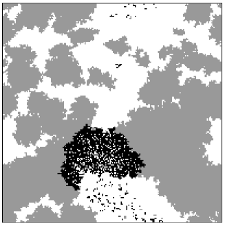
FIG. 12.: Typical stationary state configuration of preys (grey) and predators (black) on a 200 $\times$ 200 lattice at $\lambda_{a}=0.9$ and $\lambda_{b}=100$. The white parts represent the empty sites. The picture shows the beginning of the invasion of the pure prey territory by predators, which were screened by empty sites before.

One can also derive an approximate formula for the position of the phase boundary between the non-oscillatory and the prey phase $\lambda_{b}^{*}(\lambda_{a})$. For $\lambda_{a}\gg 1$, the system is almost full of preys ($a\approx 1$) and, in some sense, the dynamics of the predators is close to that of the CP. The predators die at rate 1 and spread at rate $\lambda_{b}$, but they cannot enter into the empty sites. One can introduce an effective $\tilde{\lambda_{b}}$ and describe the process as a CP, namely, the predators can enter any neighboring site at this rate. As the number of empty sites is proportional to leading order to $1/\lambda_{a}$, the effective parameter should be $\tilde{\lambda_{b}}=\lambda_{b}-c/\lambda_{a}$, where $c$ is a fitting parameter. As this CP displays a phase transition at $\tilde{\lambda_{b}}=\lambda_{CP}^{*}$, in terms of the original parameter the transition occurs at $\lambda_{b}^{*}(\lambda_{a})=\lambda_{CP}^{*}+c/\lambda_{a}$. This conjecture is in excellent agreement with the simulation data for $\lambda_{a}>0.5$ with $c=1.28(3)$ (see Fig. 3).

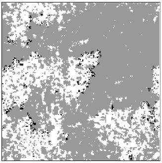
FIG. 13.: The same as Fig. 12 but for $\lambda_{a}=0.2$ and $\lambda_{b}=5$. Note, that the predators invade only the fully dense prey areas on both figures.

For $\lambda_{b}\gg 1$ the new prey sites are usually immediately occupied by predators as well. However, with a small but finite probability, a predator site can disappear before the predators spread to the new born prey site, and in this way, a prey site can be left alone and grow (similarly to the Eden model [22]). This rare event is negligible when the predator density is large enough and a prey island cannot grow for long periods of time. Practically this is the case for $\lambda_{a}>\lambda_{CP}^{*}$. In this case, the number of prey sites is negligible small, and the predator sites behave as the infected species in the CP. One can see on the Fig. 7 and 8, that for $\lambda_{b}=100$ the two densities ($a\approx b$) are equal to that of the CP if $\lambda_{a}>\lambda_{CP}^{*}$. However, in the vicinity of $\lambda_{CP}^{*}$ the densities are low, which allows an isolated prey island to grow for a long time. If $\lambda_{a}<\lambda_{CP}^{*}$ the predator islands are shrinking and, if $\lambda_{a}$ and $L$ are not too small, they can survive until a growing prey island reaches one of them. At this moment, the predators invade very quickly the prey territory and increase their population size (see Fig. 12). These new predator sites start to die out leaving a few prey sites alone, and the whole procedure starts again. This mechanism insures the survival of the predators much bellow the CP critical density and results in oscillations in the population sizes.

For $\lambda_{b}>\lambda_{b}^{T}$, but not too large, the qualitative picture is slightly different. As one can observe on Fig. 13, groups of predators are wandering through the system towards prey-dense areas. If two fronts of predators meet they usually stop moving and the local population of predators starts shrinking. The oscillations are maintained in a somewhat similar way than for the $\lambda_{b}\gg 1$ case: these predators can only survive if the preys become dense around them. This is more probable for larger values of $\lambda_{a}$, and it is also clear that the predators have a better chance to survive in larger systems.

According to the above statements, the key point in the underlying mechanism of oscillations is the existence of blocked predator islands which are located and trapped in sparse prey areas. Indeed, blocked predators in sparse prey areas result in growing prey populations; however, the resulting dense prey population allows predators to move and predate again. This mechanism drives back the system to the beginning of the loop. Clearly, predators can only be trapped in sparse prey areas if $\lambda_{a}$ is smaller or of the order of the death rate, 1. This explains the location of the oscillatory region. Note, that the above argument is based on the spatial nature of the system, suggesting that the spatially extended character is fundamental for the existence of such prey-predator type of oscillations.

This mechanism also provides a qualitative understanding of the key properties of the system. The trapped predators can invade the prey area only when the preys are dense enough again, which takes a time proportional to $1/\lambda_{a}$, and leads to $\omega\sim\lambda_{a}$. According to the simulations the correlation length, $\xi$, increases with decreasing $\lambda_{a}$. Indeed, as $\lambda_{a}$ decreases, the trapped predators have to wait longer to escape, hence fewer groups of predators survive. This increases the distance between the groups, resulting in larger prey islands, which average size is proportional to $\xi_{a}$.

When the correlation length is of the order of the system size, there are islands of preys of typical size L, extruding the predators out of the system. Hence, the condition $\xi_{a}\sim L$ characterizes the phase boundary between the oscillatory and the prey phase. On the other hand, a correlation length of order one ($\xi_{a}\sim 1$), means that the noise dominates the system. Thus, $\xi_{a}\sim 1$ characterizes the boundary between the oscillatory and the non-oscillatory region of the coexistence phase.

As shown by the study of the time dependent correlations, domains separated by a distance larger than $\xi_{a}$ oscillate asynchronously around a constant value with the same frequency, $\omega(\lambda_{a},\lambda_{b})$. According to this picture, one can derive a more quantitative description for the oscillatory region. Let us assume that for $1\ll\xi_{a}\ll L$, the global densities of each species can be written as the sum of local coarse-grained densities at a typical length scale $\xi_{a}$. Moreover, we assume that all these local densities oscillate with the same frequency but a different phase, $\alpha_{l}$. In general, the amplitude of the local oscillations should depend on the parameters $\lambda_{a}$ and $\lambda_{b}$. However, as one can observe on Fig. 12 and 13, the predators can only enter an almost fully dense prey area and the predator fronts leave an almost empty field behind them. Hence, as suggested by the numerical simulations, everywhere in the oscillatory region, the local amplitude for the prey density can be considered as a constant, $d$. Thus

$$a(t)=a^{s}+d\left(\frac{\xi}{L}\right)^{2}\sum_{l=1}^{\left(\frac{L}{\xi}\right)^{2}}\sin(\omega t+\alpha_{l})~{}.$$ (25)

Supposing that the $\alpha_{l}$ values change much more slowly than $\omega$, $a(t)$ shows a simple $\sin$ behavior for long periods of time (see Fig. 4). Thus, for $a(t)$ one can derive the value of the density fluctuations, $\chi_{a}$, and the amplitude of these oscillations, $A_{a}$, using (12) and (22), and take the average over all the possible $\alpha_{l}$ configuration taken from a flat distribution. This procedure reproduces the result of Eq. (23) up to a multiplicative factor in front of the correlation length.

VI Conclusions

We have studied a two dimensional prey-predator model, (size $L\times L$), which exhibits a rich stationary state phase diagram. A particular attention has been payed to the study of finite size effects, and we were able to draw clear cut conclusions concerning the behavior of the model both for $L$ finite as well as for the limit $L\to\infty$.

Three kinds of stationary states can be reached according to the values of the control parameters : a pure prey state, and two coexisting prey-predator ones with and without oscillations. Two different kinds of second order transitions were found when going into the prey absorbing phase. The transition between oscillatory and non-oscillatory coexistence phase is, in fact, a cross-over between two asymptotic regimes characterized by a very small and a large correlation length respectively. In the oscillatory regime, scaling relations were established between several physical quantities.

A qualitative explanation for the existence of such oscillatory regime is given, pointing out the crucial role of the spatial extension of the system. Indeed, the frequency of the oscillations is determined locally due to the dynamics related to blocked predator islands in sparse prey areas. Regions of linear size $\xi_{a}$ oscillate with the same frequency but with different phases. This explains the decreasing amplitude of oscillations with increasing system size. On the other hand, slowly changing phases result periodic oscillations in the overall prey density for long periods of time. Moreover, for suitable choices of the control parameters one can have synchronized oscillations with finite amplitude across arbitrary large systems. Thus we think that our simple model could offer a qualitative explanation for the behavior of the lynx population problem described in Sec. I.

- [1] A.J. Lotka, Proc. Natl. Acad. Sci. U.S.A. 6, 410 (1920).
- [2] V. Volterra, “Leçons sur la théorie mathématique de la lutte pour la vie”, (Gauthier-Villars, Paris 1931).
- [3] N.S. Goel, S.C. Maitra and E.W. Montroll, “Nonlinear models of interacting populations”, (Academic Press, New-York, 1971).
- [4] B. Blasius, A. Huppert and L. Stone, Nature 399, 354 (1999) and references therein.
- [5] C. Elton and M. Nicholson, J. Anim. Ecol. 11, 215 (1942).
- [6] P. Rohani, R.M. May and M.P. Hassell, J. Theor. Biol. 181, 97 (1996); “Modeling Spatiotemporal Dynamics in Ecology”, ed. by J. Bascompte and R. V. Solé, (Springer, 1998).
- [7] V.A.A. Jansen, OIKOS 74, 384 (1995).
- [8] A.T. Bradshaw, L.L. Moseley, Physica A 261 107 (1998)
- [9] J.E. Satulovsky and T. Tomé, Phys. Rev. B 49, 5073 (1994).
- [10] N. Boccara, O. Roblin and M. Roger, Phys. Rev. E 50, 4531 (1994).
- [11] A. Provata, G. Nicolis and F. Baras, J. Chem. Phys. 110, 8361 (1999).
- [12] K. Tainaka, J. Phys. Soc. Japan, 57 2588 (1988).
- [13] A. Pekalski and D. Stauffer, Int. Jour. Mod. Phys. C6, 777 (1998).
- [14] A. Lipowski, Phys. Rev. E 60, 5179 (1999).
- [15] A. Lipowski and D. Lipowska, Physica A 276, 456 (2000).
- [16] B. Chopard, M. Droz and S. Galam, to appear in Eur. Phys. Jour. B (2000).
- [17] T. E. Harris, Ann. Probab. 2, 969 (1974); T.M. Liggett, “Interacting particle systems”, (Springer, 1985).
- [18] W. Kinzel, in “Percolation structures and concepts”, Annals of the Israel Physical Society, 5, 425 (1983).
- [19] P. Grassberger, J. Phys. A 22, 3673 (1989).
- [20] I. Jensen, J.Phys. A 29, 7013 (1996).
- [21] H.K. Janssen, Z. Phys. B 42, 151 (1981); P. Grassberger, Z. Phys. B 47, 365 (1982).
- [22] M. Eden, in:”Symposium on Information Theory of Biology”, Pergamon Press, New York, (1958).