Abstract

In this paper we test computationally the performance of $CAPM$ in an evolutionary setting. In particular we study the stability of wealth distribution in a financial market where some traders invest as prescribed by $CAPM$ and others behave according to different portfolio rules. Our study is motivated by recent analytical results that show that, whenever a logarithmic utility maximiser enters the market, traders who either “believe” in $CAPM$ and use it as a rule of thumb for their portfolio decisions, or are endowed with genuine mean-variance preferences, vanish in the long run. Our analysis provides further insights and extends these results. We simulate a sequence of trades in a financial market and: first, we address the issue of how long is the long run in different parametric settings; second, we study the effect of heterogeneous savings behaviour on asymptotic wealth shares. We find that $CAPM$ is particularly “unfit” for highly risky environments.

JEL Classification C61, D81, G11

Keywords Evolution; portfolio rules; $CAPM$; Kelly criterion.

1 Introduction

A major part of research in financial economics is aimed at improving our understanding of how investors make their portfolio decisions and hence of how asset prices are determined. In this paper we contribute to that research adopting a dynamic approach, where investors’ wealth endowments and portfolio rules evolve in time.

We adopt here an evolutionary framework to address the issues of fitness and survival in financial markets, where traders differ in portfolio rules and/or savings behaviour. We build a simple framework that allows us to simulate a long sequence of trades in a competitive financial market and to test computationally the asymptotic wealth distribution of traders who follow heterogeneous portfolio rules. In particular we concentrate our analysis on the interaction between two types of traders: traders who use (the traditional version of) $CAPM$ as a rule of thumb for their portfolio decisions and traders who make portfolio choices maximising a logarithmic utility function.

The choice of this particular focus of analysis is motivated by an old debate and a recent strand of literature. Despite the fact that its restrictive assumptions have often been criticised and its predictive power has been challenged by numerous contribution in empirical finance (see for example Fama and French[4, 5]), the mean variance approach is a standard in financial economics, and its main corollary in asset pricing, the Sharpe-Lintner-Mossin Capital Asset Pricing Model , has been viewed as one of the “major contributions of academic research in the postwar era” (Jagannathan and Wang [9], p.4). Since a seminal article by Kelly [10], financial economists and applied probability theorists have been debating on the normative appeal of logarithmic utility maximisation as opposed to the mean-variance approach in financial markets. Several contributors have expressed their dissatisfaction with the mean-variance approach and argued that a rational investor with a long time horizon should instead maximise the expected rate of growth of his wealth. The portfolio choice that this type of behaviour implies is equivalent to that prescribed by a logarithmic utility function (the so called “Kelly criterion”). Central to the debate was the claim that maximising a logarithmic utility function would be a “more rational” objective to follow for a trader with a long time horizon. This claim has been strongly opposed by Merton and Samuelson [13] and Goldman [7], who stressed the obvious contradiction that lies in arguing that rational traders should maximise a given utility function, possibly different from their own.

We believe that a useful contribution to this debate comes by the adoption of an evolutionary technique. By showing that logarithmic utility maximisers accumulate more wealth than $CAPM$-traders we certainly do not prove that they are more rational (or happier) than their mean-variance opponents. However we may gain a better understanding of the reasons for the support of logarithmic utility maximisation that originated the debate.

We do not attempt here a review on the literature on evolution and market behaviour. Instead we concentrate on the more self-contained strand of literature to which this paper specifically contributes. In particular, we focus on the literature that aims at studying long run financial market outcomes as the result of a process akin to natural selection. In a seminal paper Blume and Easley [2] develop an evolutionary model of a financial market and define notions of dominance, survival and extinction based on the asymptotic behaviour of traders’ wealth shares. They provide us with the most general analytical result in this strand of literature. They show that, if all traders save at the same rate and under some uniform boundedness conditions on portfolios, then there exists one globally fittest portfolio rule which is prescribed by logarithmic utility maximisation. Namely, if there is a logarithmic utility maximiser in the economy, he will dominate, determine asset prices asymptotically and drive to extinction any other trader that does not behave, at least in the long run, as a logarithmic utility maximiser.

In a different setting, where investors choose their investment rates endogenously (choosing an optimal consumption stream at the same time as an optimal sequence of portfolios), Sandroni [15] provides analytical results that seem to weaken Blume and Easley’s findings. He shows that, provided that agents’ utilities satisfy Inada conditions (and that agents’ beliefs are correct), then all traders survive. Clearly Inada conditions are crucial here as they require marginal utilities to go to infinity whenever the consumption level approaches zero. A rational trader that can also choose his investment intensity would avoid extinction by suitably modifying his consumption pattern.

Sciubba [16] compares the relative fitness of logarithmic and mean-variance preferences. Mean-variance preferences do not satisfy Inada conditions and prescribe portfolio weights which do not necessarily display uniform boundedness properties, so that none of the two previous frameworks directly applies. She shows that when logarithmic utility maximisers invest at the same rate as mean-variance investors, logarithmic traders dominate, determine asset prices asymptotically and drive to extinction those agents who are either endowed with mean-variance preferences, ore use their theoretical predictions ($CAPM$) as a rule of thumb. One of the sections in Sciubba [16] is indeed devoted to the study of the role of heterogeneous savings rates in the dynamics of wealth accumulation. However, the stochastic process becomes so complex in this case, that the few results that are obtainable analytically are very weak. This is where we believe that numerical computation can provide us with more insights into the problem.

Our results show that, even when we allow for heterogeneity in savings rates, dominance of logarithmic utility maximisers proves robust, at least to a certain extent. In particular, we show that logarithmic traders can “afford” to save at a lower rate than $CAPM$ traders and still dominate financial markets. When logarithmic traders dominate, the wealth share of $CAPM$ traders converges to zero exponentially fast. In particular, we find that the more risk-averse $CAPM$ traders are, the faster they vanish. Clearly when $CAPM$ traders display a savings intensity that is much higher than their opponents, then - as one would expect - they indeed dominate and drive to extinction logarithmic utility maximisers. We identify the threshold in the savings rates differential such that this “fate reversal” occurs and find that it is increasing in the variance of the dividend stream. If the dividend stream is very volatile, then the advantage of logarithmic utility maximisers with respect to $CAPM$ traders in terms of portfolio selection is higher. Hence $LOG$ traders can “afford” to save less and still dominate the market. Symmetrically, the fitness of $CAPM$ proves particularly low in environments characterised by high volatility. Should we trust what $CAPM$ prescribes when investing on Nasdaq? Probably not.

2 The Model

A detailed description of the model is to be found in Sciubba [16]. Here we summarise its main features. Time is discrete and indexed by $t=0,1,2,...$. There are $S$ states of the world indexed by $s=1,2,...,S$, one of which will occur at each date. States follow an i.i.d. process with distribution $p=(p_{1},p_{2},...,p_{S})$ where $p_{s}>0$ for all $s$. There is a finite set of assets, with the same dimensionality of the set of states of nature. With little abuse of notation we index both assets and states with the same letter. Asset $s\in\left\{1,2,...,S\right\}$ pays a strictly positive dividend $d_{s}>0$ when state $s\in\left\{1,2,...,S\right\}$ occurs and $0$ otherwise. At each date there is only one unit of each asset available, so that $d_{s}$ will be the total wealth in the economy at date $t$ if state $s$ occurs. This wealth will be distributed among traders proportionately according to the share of asset $s$ that each of them owns. Let $\rho_{st}$ be the market price of (one unit of) asset $s$ at date $t$. There is a heterogeneous population of long-lived agents in this economy, indexed by $i\in\left\{1,2,...,I\right\}$. Each agent is characterised by an investment rule and an initial wealth endowment. Agent $i$’s investment rule is $\left\{\delta_{t}^{i},\alpha_{t}^{i}\right\}_{t=0}^{\infty}$ where $\delta_{t}^{i}$ denotes agent $i$’s investment rate at date $t$ (i.e. the percentage of wealth endowment at date $t$, $e_{t}^{i}$, that $i$ invests at date $t$) and $\alpha_{t}^{i}$ is a vector that describes agent $i$’s portfolio choice at date $t$ (i.e. the vector of portfolio weights in the $S$ available assets $\left\{\alpha_{st}^{i}\right\}_{s=1}^{S}$ for agent $i$ at date $t$). Agent $i$’s initial wealth endowment is denoted by $e_{0}^{i}$. The tuple $\left(e_{0}^{i},\left\{\delta_{t}^{i},\alpha_{t}^{i}\right\}_{t=0}^{\infty}\right)$ constitutes a complete description of agent $i$. At each date $t$, agent $i$ invests a portion $\delta_{t}^{i}$ of his wealth endowment $e_{t}^{i}$, in the $S$ available assets. We denote by $w_{t}^{i}$ the total amount invested by trader $i$ at date $t:$

$$w_{t}^{i}=\delta_{t}^{i}e_{t}^{i}$$ (1)

Aggregate total investment will be equal to aggregate expenditure in assets. Since there is only one unit of each asset available, then clearly:

$$\sum_{s=1}^{S}\rho_{st}=\sum_{i=1}^{I}w_{t}^{i}=w_{t}$$ (2)

Equation (2) provides us with a convenient normalisation for prices. We can, in fact, call $\pi_{st}$ the normalised market price of asset $s$ at date $t$ and define it as follows:

$$\pi_{st}\equiv\frac{\rho_{st}}{\sum_{s=1}^{S}\rho_{st}}=\frac{\rho_{st}}{w_{t}}$$ (3)

Finally define: $\pi_{t}\equiv\left(\pi_{1t},\pi_{2t},...,\pi_{St}\right)$. In equilibrium, prices must be such that markets clear, i.e. total demand equals total supply. Agent $i$’s demand for asset $s$ will be equal to agent $i$’s expenditure in asset $s$, $\alpha_{st}^{i}\,w_{t}^{i}$, divided by the market price of asset $s$, $\rho_{st}$. In the aggregate:

$$\sum_{i=1}^{I}\frac{\alpha_{st}^{i}\,w_{t}^{i}}{\rho_{st}}=1$$ (4)

Rewriting equation (4) we get:

$$\rho_{st}=\sum_{i=1}^{I}\alpha_{st}^{i}\,w_{t}^{i}$$ (5)

and using our price normalisation:

$$\pi_{st}=\sum_{i=1}^{I}\alpha_{st}^{i}\,\varepsilon_{t}^{i}$$ (6)

where $\varepsilon_{t}^{i}$ denotes the investment share of agent $i$ at date $t$:

$$\varepsilon_{t}^{i}=\frac{w_{t}^{i}}{w_{t}}$$ (7)

and also measures the “presence” of trader $i$ in financial markets and his “importance” in determining asset prices.

2.1 The Dynamics

We now ask what is the period to period dynamics of trader $i$’s investment share. This will allow us to follow the evolution of his “presence” in financial markets and of his “importance” in determining market outcomes, namely asset prices. Suppose that state $s$ occurs at date $t$: asset $s$ pays a dividend $d_{s}$ while all other assets pay zero. The total wealth in the economy, $d_{s}$, gets distributed to traders according to the share of asset $s$ that each of them owns. In particular, the investment income of trader $i$ - that also constitutes his wealth endowment for period $t+1$ - is equal to the following:

$$e_{t+1}^{i}=\frac{\alpha_{st}^{i}w_{t}^{i}}{\rho_{st}}d_{s}$$ (8)

Aggregate wealth endowment at date $t+1$ is equal to the total payout of asset $s$:

$$e_{t+1}=\sum_{i=1}^{I}e_{t+1}^{i}=\sum_{i=1}^{I}\frac{\alpha_{s}^{i}w_{t}^{i}}{\rho_{st}}d_{s}=d_{s}$$ (9)

In period $t+1$ trader $i$ invests a fraction $\delta_{t+1}^{i}$ of his wealth endowment:

$$w_{t+1}^{i}=\delta_{t+1}^{i}e_{t+1}^{i}=\delta_{t+1}^{i}\frac{\alpha_{st}^{i}d_{s}}{\rho_{st}}w_{t}^{i}$$ (10)

In the aggregate:

$$w_{t+1}=\sum_{i=1}^{I}w_{t+1}^{i}=\sum_{i=1}^{I}\delta_{t+1}^{i}\frac{\alpha_{st}^{i}w_{t}^{i}}{\rho_{st}}d_{s}=\sum_{i=1}^{I}\delta_{t+1}^{i}\frac{\alpha_{st}^{i}w_{t}^{i}}{\rho_{st}}e_{t+1}$$ (11)

In order to formulate (10) in terms of wealth shares, it is useful to define the market average investment rate $\delta_{t+1}$ as:

$$\delta_{t+1}=\sum_{i=1}^{I}\delta_{t+1}^{i}\frac{\alpha_{st}^{i}w_{t}^{i}}{\rho_{st}}$$ (12)

so that (11) can be rewritten as:

$$w_{t+1}=\delta_{t+1}e_{t+1}$$ (13)

Dividing (10) by (11) we obtain investment shares:

$$\varepsilon_{t+1}^{i}=\frac{w_{t+1}^{i}}{w_{t+1}}=\frac{\delta_{t+1}^{i}\alpha_{st}^{i}d_{s}}{\delta_{t+1}\rho_{st}e_{t+1}}w_{t}^{i}$$ (14)

Finally, using (9) and our price normalisation, we obtain:

$$\varepsilon_{t+1}^{i}=\frac{\delta_{t+1}^{i}\alpha_{st}^{i}}{\delta_{t+1}\pi_{st}}\varepsilon_{t}^{i}$$ (15)

Equation (15) describes the period to period dynamics of the investment share of trader $i$. It implies that the “impact” of trader $i$ on financial markets follows a fitness-monotonic dynamic: trader $i$’s investment share will increase if he invests more than the market on average and if he scores, with his investments, a payoff which is higher than the average population payoff. In fact, if state $s$ occurs at date $t$, $\alpha_{st}^{i}$ and $\pi_{st}$ give us a measure of trader $i$’s payoff (his bet on the lucky asset) and of the average population payoff respectively. Following the definition given by Blume and Easley [2], in order to establish whether trader $i$ survives or vanishes, we consider the asymptotic value of his investment share and we check whether it is bounded away from zero or not. When trader $i$’s investment share converges to zero, his significance in determining market outcomes vanishes and he effectively disappears from the market. When trader $i$’s investment share stays bounded away from zero, then he contributes to determine asset prices (also asymptotically) and we will say that, as a trader, he survives. The process described by eq.(15) is too complex to be studied analytically in a very general case. In fact, even under the restriction that all shocks are i.i.d., asset prices and market savings rates depend on the whole sequence of past history, and the law of large numbers does not automatically help us with a solution. As we argued in the introduction, this is why we believe that numerical analysis can help to obtain further insights into the problem.

2.2 Types of Traders

As in Sciubba [16], we will consider the interaction between two different types of traders. The first type of agents is given by investors who believe in $CAPM$ and use it as a rule of thumb : at the beginning of each time period, they observe payoffs and market prices and work out the composition of the market and the risk-free portfolios. Finally, according to their degree of risk aversion they choose their preferred combination between the two. At date $t$, $CAPM$ investors choose $\gamma_{t}\in\left[0,1\right]$ and invest in asset $s$ a portion $\alpha_{st}^{CAPM}$ of their portfolio such that:

$$\alpha_{st}^{CAPM}=\gamma_{t}\alpha_{st}^{F}+\left(1-\gamma_{t}\right)\alpha_{st}^{M}$$ (16)

where:

$$\alpha_{st}^{F}\equiv\frac{\rho_{st}/d_{s}}{\sum_{z}\rho_{zt}/d_{z}}=\frac{\pi_{st}/d_{s}}{\sum_{z}\pi_{zt}/d_{z}}$$ (17)

and

$$\alpha_{st}^{M}\equiv\frac{\rho_{st}}{\sum_{z}\rho_{zt}}=\pi_{st}.$$ (18)

The second type of traders is given by investors who are endowed with a logarithmic utility function (type $LOG$) and who actually maximise the growth rate of their wealth share and invest according to a “simple” and time invariant portfolio rule:

$$\alpha_{st}^{LOG}=p_{s}$$ (19)

More generally, at each date $t$, a rational trader $i$ will choose $\left\{\alpha_{st}^{i}\right\}_{s=1}^{S}$ so as to maximise:

$$\sum_{s=1}^{S}p_{s}u^{i}\left(\frac{\alpha_{st}^{i}w_{t}^{i}}{\rho_{st}}d_{s}\right)$$ (20)

subject to the constraint that investment expenditure at each date is less than or equal to the amount of wealth saved in the previous period. If $u^{i}\left(\cdot\right)$ is logarithmic, it follows that $\alpha_{st}^{L}=p_{s}$. We will denote by $\delta_{t}^{CAPM}$ and $\delta_{t}^{LOG}$ the investment rates of traders who believe in $CAPM$ and logarithmic utility maximisers respectively.

3 Computer Simulation and Numerical Results

Recall eq.(6) where normalised prices are expressed as a weighted average of portfolio rules. In the setting that we consider, where $CAPM$ and $LOG$ traders interact, eq.(6) becomes

$$\pi_{st}=\varepsilon_{t}\alpha^{LOG}_{st}+(1-\varepsilon_{t})\alpha^{CAPM}_{st}$$ (21)

where $\varepsilon_{t}$ denotes the investment share of $LOG$ traders and $(1-\varepsilon_{t})$ denotes the investment share of $CAPM$ traders. By substituting eq.(16) and eq.(19) in eq.(21) one has

$$\pi_{st}=\varepsilon_{t}p_{s}+(1-\varepsilon_{t})(\gamma\frac{\pi_{st}}{d_{s}}\frac{1}{\sum_{z=1,N}\frac{\pi_{zt}}{d_{z}}}+(1-\gamma)\pi_{st}).$$ (22)

We solve the above equation through iteration by a numerical technique called “relaxation”. Namely, we start from a trial value for $\pi_{st}$, we compute a new value through the above equation and then we iterate this procedure until a fixed point is reached. In other words, if we call $\tau$ the time of the iteration our numerical code computes the quantity

$$\pi_{st}^{\tau+1}=\varepsilon_{t}p_{s}+(1-\varepsilon_{t})(\gamma\frac{\pi_{st}^{\tau}}{d_{s}}\frac{1}{\sum_{z=1,N}\frac{\pi_{zt}^{\tau}}{d_{z}}}+(1-\gamma)\pi_{st}^{\tau})$$ (23)

and then it looks for the fixed point solution $\pi_{st}^{\infty}$ that is achieved for all the $\tau>\tau^{*}$ for which $|\pi_{st}^{\tau^{*}+1}-\pi_{st}^{\tau^{*}}|$ is less than a tolerance parameter fixed in advance for all the assets $s$. This fixed point is the numerical solution of eq.(23). Since it has been demonstrated that this solution exists and is unique [16], it is possible to show that the above method gives a numerical value of the solution with a desired precision bounded only by computation time. In our simulations we stop the iteration when the relative precision of asset prices is lower than $10^{-5}$. At this point we run two sets of simulations. The first set aims at detecting the time of convergence of the stochastic process given by the wealth shares. The second set of simulations aims at checking the robustness of $LOG$ dominance results to heterogeneity in savings rates.

The first numerical check is devoted to study the average time one can expect $CAPM$ traders to survive in a competition with the others. We run a Fortran code that simulates a real evolution in a market with $CAPM$ traders and $LOG$ traders. We consider a market where 100 assets are repeatedly traded, so that $S=100$. We assume that the probability distribution over the states of nature is uniform, so that $p_{s}=1/S,\,\forall s$. We assume that dividends are randomly drawn from a normal distribution $N(\mu,\sigma)$ with the mean to variance ratio large enough to guarantee that virtually every asset pays a positive payoff. We set the initial investment shares for the two types of traders to be equal. None of the qualitative results that we obtain in the simulation are driven by our choice of parameters and probability distributions. We run our simulations under the assumption (as in Sciubba [16] and Blume and Easley [2]) that both types of traders save at the same rate. Time step after time step the code generates pseudo-random numbers that identify states of nature. After each draw, prices are computed through “relaxation”, the dividends are distributed and the investment shares of the traders are refreshed. Eventually the investment share of $CAPM$ traders becomes lower than a certain threshold, sufficiently small such that we can conclude that $CAPM$ traders are extinct. We then store in the computer the time at which this threshold is reached and we start again with a new realisation of the same market. Given the same initial conditions in the market, we collect up to $15000$ different realisations of this competition between traders. The various realisations differ because of the randomness in the draw of the states of nature. In all the runs $CAPM$ traders see their investment shares reduced until extinction takes place. This result confirms the theoretical findings. Furthermore, through the extinction times recorded by the computer code, we are also able to measure the density function describing the probability that $CAPM$ traders survive up to a time $t$ in a competition with $LOG$ traders. The unit of time is given by the draw of a state of nature. That is, $t=5$ means that after the initial condition $5$ states of nature have been drawn in the market, and the $5$ corresponding assets paied their dividends. The main result is that the density function is exponential. The probability for a $CAPM$ trader to survive decreases with time according to

$$P(t)dt=Ae^{-Ct}dt.$$ (24)

We also run different simulations by changing the parameter $\gamma$ of the model, that measures the risk-aversion of $CAPM$ traders. The result is that the more risk-averse the $CAPM$ traders are, the faster their wealth share converges to zero. The economic intuition for this result lies in the fact that a higher degree of risk-aversion implies that the portfolio of $CAPM$ is tilted towards the risk-free rather than towards the market portfolio, where the most successful trading rules are represented. In this setting, a $CAPM$ trader with an extremely low risk-aversion, and hence a value of $\gamma$ approximately equal to zero, would indeed survive.

Our simulations show that exponential decay is robust with respect to the values of $\gamma$ used. The functional form that can be hypothesised for such a decay is of the form

$$P(t)=Ae^{-Bt\gamma^{2}}$$ (25)

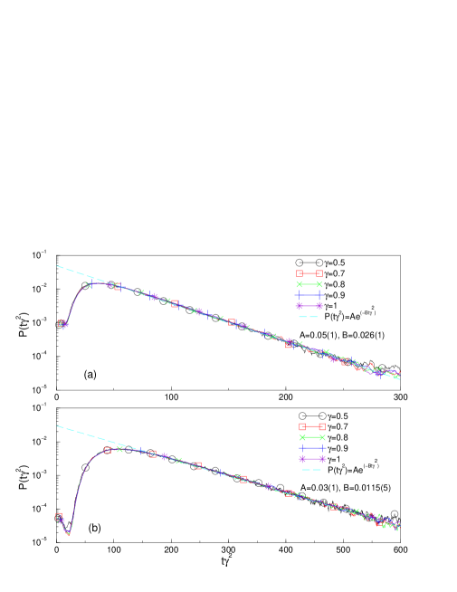
Figure 1: Different density functions for the lasting probability for different values of $\gamma$. In the picture above a threshold of $5\%$ of aggregate wealth has been adopted to claim traders’ extinction. In the picture below we used a threshold ten times lower. This change affects only the scale of time and the parameters of the fit, but it does not affect the form of the distribution.

One can test this assumption by rescaling the different data. Namely in each simulation, if we multiply the value of time by the value of $\gamma^{2}$ used in that run, we should obtain different functions $P^{\prime}(t^{\prime})$ (where $t^{\prime}=t\gamma^{2}$) all behaving in the same way. In particular these data obtained through simulations with different values of $\gamma$ should collapse together. This technique note as “collapse plot” is shown in Fig.1. In the upper part of the figure we plot the data relative to $\gamma=0.5,0.7,0.8,0.9,1$ testing the good validity of our assumption. We also run another set of simulations, by changing the threshold at which the $CAPM$ trader is considered extinct. By passing to a threshold of $0.5\%$ of the total wealth shares from the $5\%$ previously used, we noticed as expected a shift of the distribution to longer times. Nevertheless, qualitatively we obtain the same behaviour shown in the lower part of Fig.1. In both cases (above and below) the extimated exponential distribution is indicated by a dashed line.

In the second set of simulations we consider the situation in which the savings rates used by the two types of traders differ. In particular, we ask if $LOG$ traders can survive and eventually dominate over $CAPM$ traders that save at a higher intensity. We run simulations of the financial market described in the previous section, in this case under the assumption that traders have heterogeneous savings rates. Our aim is to check whether $LOG$ dominance results are robust when $CAPM$ traders save at a higher rate than logarithmic utility maximisers. As in the previous set of simulations, we consider a market where 100 assets are repeatedly traded, such that $S=100$. Again, we assume that the probability distribution over the states of nature is uniform, so that $p_{s}=1/S,\,\forall s$. We assume that dividends are randomly drawn from a normal distribution $N(\mu,\sigma)$ with the mean to variance ratio large enough to guarantee that virtually every asset pays a positive payoff. We set the initial wealth shares for the two types of traders to be equal. Finally we normalise the savings rate of $CAPM$ traders to be equal to one.

Fig. 2 shows the lowest value for logarithmic utility maximisers’ savings rate that still allows $LOG$ traders to dominate (averaged across $1000$ different simulations), for different values of the variance $\sigma$ of the distribution of dividends, which measures the volatility of the dividend stream. More particularly, we introduce the quantity $\Delta$ representing the maximum difference in saving rates between $CAPM$ and $LOG$ that still allows $LOG$ traders to dominate. Also in this case we apply the technique of the collapse plot in order to show that the threshold at which $LOG$ traders commence to dominate depends on the ratio $\sigma/\mu$. We can interpret the graph in figure 2 as dividing the $\sigma$, $\Delta$ plane in two regions: in the area (a) below the graph, logarithmic utility maximisers dominate and drive to extinction $CAPM$ traders; in the area (b) above the graph, $CAPM$ traders dominate and drive to extinction logarithmic utility maximisers. From our results it appears that the dominance of logarithmic utility maximisers is robust to heterogeneity in savings rates, at least to a certain extent. In fact we obtain that $LOG$ traders dominate and drive $CAPM$ traders to extinction even when the latter display a higher savings rate (provided that it is not much higher). This difference provides us with an immediate measure of the advantage of $LOG$ traders with respect to $CAPM$ traders in terms of portfolio rules. We find that the higher the volatility of the dividend stream, the higher is the advantage of logarithmic utility maximisers over $CAPM$ traders. In particular, the threshold level for the $LOG$ traders’ savings rate appears to be a function of the mean to variance ratio of the probability distribution of the dividends that assets pay. The economic intuition of this result lies in the fact that, with a large variance of dividends, the behaviour prescribed by a logarithmic utility function differs greatly from the behaviour prescribed by CAPM. Think of the following example. Suppose that investors can place bets on two lotteries that pay positive prizes with equal probability: lottery ”Rich” pays 1 million dollars with probability 1/2 and lottery ”Poor” pays 1 single dollar whenever lottery ”Rich” does not pay. A LOG investor would place equal bets on both lotteries. On the contrary, a CAPM trader (and any trader, in fact, that maximises the expected value of an increasing function of his wealth level, rather than rate of growth) would place a higher bet on the ”Rich” lottery than on the ”Poor” one. The divergence between his bets would be increasing in the difference between the two lotteries’ prizes. As a result, the distance between the bets that LOG investors and CAPM investors would place is also increasing in the discrepancy between lotteries’ payoffs. A higher variance of dividends implies that, in different states of nature, very high payoffs are paid as well as very low ones, and results in a higher divergence of portfolio choices between the two types of investors.

4 Conclusion

In this paper we test computationally the performance of $CAPM$ in an evolutionary setting. In particular we study the asymptotic wealth distribution across two types of traders that compete on financial markets: traders who invest as prescribed by $CAPM$ and traders who maximise the expected value of a logarithmic utility function of wealth. Our study provides further insights and extends some recent analytical results (see [16]) that prove that the wealth share of $CAPM$ traders converges almost surely to zero, when a logarithmic utility maximiser with a savings rate at least as large as the savings rate of $CAPM$ traders, enters the market. We run two sets of simulation addressing two related, but separate, issues. First, we look at the time of convergence of the stochastic process given by the wealth share dynamics. We find that, when savings rates are identical across the two types of traders, the wealth share of $CAPM$ investors decreases exponentially fast towards zero. We also find that the degree of risk-aversion of $CAPM$ traders has a role in determining the speed of convergence: the more risk-averse the $CAPM$ traders, the faster their wealth share converges to zero. Second, we check the robustness of the analytical result in Sciubba [16] to heterogeneity in savings rates. We find that $LOG$ investors dominate even when their savings rate is lower (but not too much lower) than the savings rate of $CAPM$ traders. We compute the maximum difference between the savings rates of the two types of investors that still allows $LOG$ traders to dominate and drive to extinction all those who choose their portfolio according to what $CAPM$ prescribes. We argue that the difference between savings rates so computed can serve as a measure of the fitness of logarithmic utility maximisation with respect to $CAPM$ and we find that it is increasing in the variance of the dividend stream. Our results seem to suggest that, from an evolutionary perspective, if it is true that $CAPM$ could perform almost as satisfactorily as logarithmic utility maximisation in markets with low volatility, it proves particularly unfit for highly risky environments.

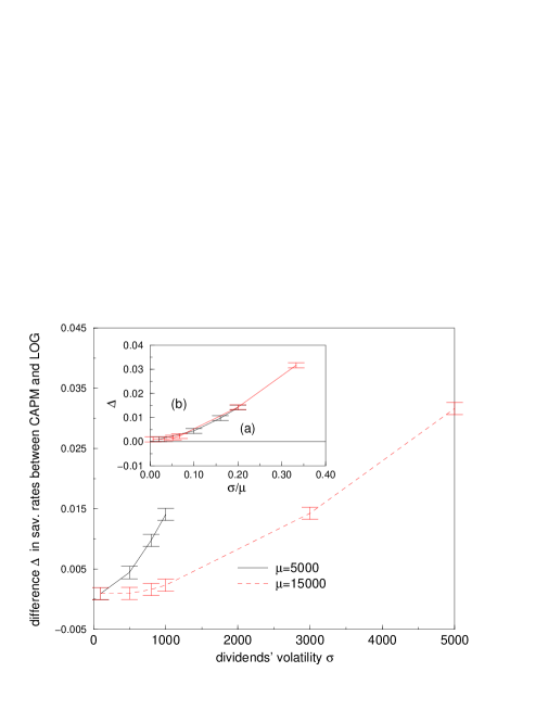
Figure 2: Values of $\Delta$ (the maximum difference between the savings rates of $CAPM$ and $LOG$ that still allows $LOG$ traders to dominate), with respect to the dividends’ volatility $\sigma$.

References

- [1] Algoet, Paul H., and Thomas M.Cover (1988): “Asymptotic Optimality and Asymptotic Equipartition Properties of Log-Optimum Investment”, Annals of Probability16, 876-898.
- [2] Blume, Lawrence E., and David Easley (1992): “Evolution and Market Behaviour”, Journal of Economic Theory 58, 9-40.
- [3] Breiman, Leo (1961): “Optimal Gambling Systems for Favorable Games”, in: Proceedings of the Fourth Berkeley Symposium, University of California Press.
- [4] Fama, Eugene F. and Kenneth R. French (1996): “Multifactor Explanations of Asset Pricing Anomalies”, Journal of Finance 51, 55-88.
- [5] Fama, Eugene F. and Kenneth R. French (1996): “The is Wanted, Dead or Alive”, Journal of Finance 51, 1947-1958.
- [6] Finkelstein, Mark, and Robert Whitley (1981): “Optimal Strategies for Repeated Games”, Advanced Applied Probability 13, 415-428.
- [7] Goldman, M.Barry (1974): “A Negative Report on the ‘Near Optimality’ of the Max-Expected-Log Policy as Applied to Bounded Utilities for Long Lived Programs”, Journal of Financial Economics 1, 97-103.
- [8] Hakansson, Nils H. (1971): “Multi-Period Mean-Variance Analysis: Toward a General Theory of Portfolio Choice”, Journal of Finance 26, 857-884.
- [9] Jagannathan, Ravi, and Zhenyu Wang (1996): “The Conditional and the Cross-Sections of Expected Returns”, Journal of Finance 51, 3-53.
- [10] Kelly, J.L. (1956): “A New Interpretation of Information Rate”, Bell System Technical Journal 35, 917-926.
- [11] Latane, Henry A. (1959): “Criteria of Choice among Risky Ventures”, Journal of Political Economy 67, 144-155.
- [12] Lintner, John,(1965): “The Valuation of Risk Assets and the Selection of Risky Investments in Stock Portfolios and Capital Budgets”, Review of Economics and Statistics 43, 13-37.
- [13] Merton, Robert C., and Paul A. Samuelson(1974): “Fallacy of the Log-Normal Approximation to Optimal Portfolio Decision-Making over Many Periods”, Journal of Financial Economics 1, 67-94.
- [14] Mossin, Jan, (1966): “Equilibrium in a Capital Asset Market”, Econometrica 34, 768-783.
- [15] Sandroni, Alvaro (1999): “Do Markets Favor Agents Able to Make Accurate Predictions”, Econometrica, forthcoming.
- [16] Sciubba, Emanuela (1999): “The Evolution of Portfolio Rules and the Capital Asset Pricing Model”, DAE Working Paper n. 9908, University of Cambridge.
- [17] Sharpe, William F., (1964): “Capital Asset Prices: A Theory of Market Equilibrium under Conditions of Risk”, Journal of Finance 19, 425-442.