Single-mode delay time statistics for scattering by a chaotic cavity

Abstract

We investigate the low-frequency dynamics for transmission or reflection of a wave by a cavity with chaotic scattering. We compute the probability distribution of the phase derivative $\phi^{\prime}={\mathrm{d}}\phi/{\mathrm{d}}\omega$ of the scattered wave amplitude, known as the single-mode delay time. In the case of a cavity connected to two single-mode waveguides we find a marked distinction between detection in transmission and in reflection: The distribution $P(\phi^{\prime})$ vanishes for negative $\phi^{\prime}$ in the first case but not in the second case.

I Introduction

Microwave cavities have proven to be a good experimental testing ground for theories of chaotic scattering[1]. Much work has been done on static scattering properties, but recently dynamic features have been measured as well[2]. A key dynamical observable, introduced by Genack and coworkers[3, 4, 5], is the frequency derivative $\phi^{\prime}={\mathrm{d}}\phi/{\mathrm{d}}\omega$ of the phase of the wave amplitude measured in a single speckle of the transmitted or reflected wave. Because one speckle corresponds to one element of the scattering matrix, and because $\phi^{\prime}$ has the dimension of time, this quantity is called the single-channel or single-mode delay time. It is a linear superposition of the Wigner-Smith delay times introduced in nuclear physics[6, 7].

The probability distribution of the Wigner-Smith delay times for scattering by a chaotic cavity is known[8]. The purpose of this paper is to derive from that the distribution $P(\phi^{\prime})$ of the single-mode delay time. The calculation follows closely our previous calculation of $P(\phi^{\prime})$ for reflection from a disordered waveguide in the localized regime[9]. The absence of localization in a chaotic cavity is a significant simplification. For a small number of modes $N$ connecting the cavity to the outside we can calculate $P(\phi^{\prime})$ exactly, while for $N\gg 1$ we can use perturbation theory in $1/N$. The large-$N$ distribution has the same form as that following from diffusion theory in a disordered waveguide[4, 5], but for small $N$ the distribution is qualitatively different. In particular, there is a marked distinction between the distribution in transmission and in reflection.

II Formulation of the problem

The geometry studied is shown schematically in Figure 1. It consists of an $N$-mode waveguide connected at one end to a chaotic cavity. Reflections at the connection between waveguide and cavity are neglected (ideal impedance matching). The $N$ modes may be divided among different waveguides, for example, $N=2$ could refer to two single-mode waveguides. The cavity may contain a ferri-magnetic element as in Refs. [10, 11], in which case time-reversal symmetry is broken. The symmetry index $\beta=1$ $(2)$ indicates the presence (absence) of time-reversal symmetry. We assume a single polarization for simplicity, as in the microwave experiments in a planar cavity[2].

The dynamical observable is the correlator $\rho$ of an element of the scattering matrix $S(\omega)$ at two nearby frequencies,

$$\rho=S_{nm}(\omega+\frac{1}{2}\delta\omega)S^{*}_{nm}(\omega-\frac{1}{2}\delta\omega).$$ (1)

The indices $n$ and $m$ indicate the detected outgoing mode and the incident mode, respectively. The single-mode delay time $\phi^{\prime}$ is defined by [3, 4, 5]

$$\phi^{\prime}=\lim_{\delta\omega\to 0}\frac{\mathrm{Im}\rho}{\delta\omega I},$$ (2)

with $I=|S_{nm}(\omega)|^{2}$ the intensity of the scattered wave in mode $n$ for unit incident intensity in mode $m$. If we write the scattering amplitude $S_{nm}=\sqrt{I}{\mathrm{e}}^{i\phi}$ in terms of amplitude and phase, then $\phi^{\prime}={\mathrm{d}}\phi/{\mathrm{d}}\omega$. We will investigate the distribution of $\phi^{\prime}$ in an ensemble of chaotic cavities having slightly different shape, at a given mean frequency interval $\Delta$ between the cavity modes. For notational convenience, we choose units of time such that $2\pi/\Delta\equiv 1$.

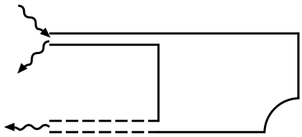
FIG. 1.: Sketch of a chaotic cavity coupled to $N$ propagating modes via one or more waveguides. The shape of the cavity is the quartered Sinai billiard used in recent microwave experiments[2].

The single-mode delay times are linearly related to the Wigner-Smith [6, 7] delay times $\tau_{1},\tau_{2},...,\tau_{N}$, which are the eigenvalues of the matrix

$$Q=-iS^{\dagger}\frac{{\mathrm{d}}S}{{\mathrm{d}}\omega}=U^{\dagger}{\mathrm{diag}}(\tau_{1},...,\tau_{N})U.$$ (3)

To see this, we first expand the scattering matrix linearly in $\delta\omega$,

$$S(\omega\pm\frac{1}{2}\delta\omega)=V^{{\mathrm{T}}}U\pm\frac{1}{2}i\delta\omega V^{{\mathrm{T}}}{\mathrm{diag}}(\tau_{1},...,\tau_{N})U.$$ (4)

Since $S$ is symmetric for $\beta=1$, one then has $V=U$. For $\beta=2$, $V$ and $U$ are statistically independent. Combination of Eqs. (1), (2), and (4) leads to [9]

$$I=|\sum_{i}u_{i}v_{i}|^{2},\hskip 4.30554pt\phi^{\prime}={\mathrm{Re}}\hskip 4.30554pt\frac{\sum_{i}\tau_{i}u_{i}v_{i}}{\sum_{j}u_{j}v_{j}},$$ (5)

$$u_{i}=U_{im},\hskip 4.30554ptv_{i}=V_{in}.$$ (6)

The distribution of the Wigner-Smith delay times for a chaotic cavity was calculated in Ref. [8]. It is a Laguerre ensemble in the rates $\mu_{i}=1/\tau_{i}$,

$$P(\mu_{1},...,\mu_{N})\propto\prod_{i<j}|\mu_{i}-\mu_{j}|^{\beta}\prod_{k}\mu_{k}^{\beta N/2}\exp(-\frac{1}{2}\beta\mu_{k})\theta(\mu_{k}).$$ (7)

The step function $\theta(x)=1$ for $x>0$ and $\theta(x)=0$ for $x<0$. It follows from Eq. (7) that $\langle\sum_{i}\tau_{i}\rangle=1$, a result that was known previously[12].

To calculate the joint distribution $P(I,\phi^{\prime})$ from Eq. (5), we also need the distribution of the coefficients $u_{i}$ and $v_{i}$. This follows from the Wigner conjecture[13], proven in Ref. [8], according to which the matrices $U$ and $V$ are uniformly distributed in the unitary group. The calculation for small $N$ is now a straightforward integration, see Sec. III. For large $N$ we can use perturbation theory, see Sec. IV.

Because of the uniform distribution of $U$ and $V$, independent of the $\tau_{i}$’s, we can evaluate the average of $\phi^{\prime}$ directly for any $N$,

$$\langle\phi^{\prime}\rangle={\mathrm{Re}}\left\langle\sum_{i}\tau_{i}\left\langle\frac{u_{i}v_{i}}{\sum_{j}u_{j}v_{j}}\right\rangle\right\rangle=\left\langle\sum_{i}\tau_{i}\frac{1}{N}\right\rangle=\frac{1}{N}.$$ (8)

We define the rescaled variable $\hat{\phi^{\prime}}=\phi^{\prime}/\langle\phi^{\prime}\rangle=N\phi^{\prime}$, that we will use in the next sections.

III Small number of modes

For $N=1$ there is no difference between the Wigner-Smith delay time and the single-mode delay time. In that case $I=1$ and $\hat{\phi^{\prime}}=\phi^{\prime}$ is distributed according to [14, 15]

$$P(\hat{\phi^{\prime}})=c_{\beta}\hat{\phi^{\prime}}^{-2-\beta/2}\exp(-\frac{1}{2}\beta/\hat{\phi^{\prime}})\theta(\hat{\phi^{\prime}}).$$ (9)

The normalization coefficient $c_{\beta}$ equals $(2\pi)^{-1/2}$ for $\beta=1$ and $1$ for $\beta=2$.

Now we turn to the case $N=2$. By writing out the summation in Eq. (5) for $I$ and $\phi^{\prime}$, one obtains $\phi^{\prime}=\tau_{+}+\alpha\tau_{-}$ with $\tau_{\pm}=\frac{1}{2}(\tau_{1}\pm\tau_{2})$ and

$$I=|u_{1}|^{2}|v_{1}|^{2}+|u_{2}|^{2}|v_{2}|^{2}+u_{1}u_{2}^{*}v_{1}v_{2}^{*}+u_{1}^{*}u_{2}v_{1}^{*}v_{2},$$ (10)

$$\alpha=(|u_{1}|^{2}|v_{1}|^{2}-|u_{2}|^{2}|v_{2}|^{2})/I.$$ (11)

To find the joint distribution $P(I,\alpha)$ we parametrize $U$ in terms of $4$ independent angles,

$$U=\left(\begin{array}[]{cc}\cos\gamma\exp(-i\alpha_{1})&\sin\gamma\exp(-i\alpha_{1}-i\alpha_{2})\\ -\sin\gamma\exp(-i\alpha_{3}+i\alpha_{2})&\cos\gamma\exp(-i\alpha_{3})\\ \end{array}\right),$$ (12)

with $\alpha_{i}\in(0,2\pi)$ and $\gamma\in(0,\pi/2)$. The invariant measure ${\mathrm{d}}\mu\propto|{\mathrm{Det}}\hskip 4.30554ptg|{\mathrm{d}}\gamma\prod_{i}{\mathrm{d}}\alpha_{i}$ in the unitary group follows from the metric tensor $g$, defined by

$${\mathrm{Tr}}\hskip 4.30554pt{\mathrm{d}}U{\mathrm{d}}U^{\dagger}=\sum_{i,j}g_{ij}{\mathrm{d}}x_{i}{\mathrm{d}}x_{j},\hskip 4.30554pt\{x_{i}\}=\{\gamma,\alpha_{1},\alpha_{2},\alpha_{3}\}.$$ (13)

The result is

$${\mathrm{d}}\mu\propto\sin 2\gamma\hskip 4.30554pt{\mathrm{d}}\gamma\prod_{i}{\mathrm{d}}\alpha_{i}.$$ (14)

The joint distribution function $P(\tau_{+},\tau_{-})$ follows from Eq. (7). For $\beta=1$ one has

$$P(\tau_{+},\tau_{-})=\frac{1}{12}|\tau_{-}|(\tau_{+}^{2}-\tau_{-}^{2})^{-4}\exp\left(-\tau_{+}(\tau_{+}^{2}-\tau_{-}^{2})^{-1}\right)\theta(\tau_{+}-|\tau_{-}|),$$ (15)

while for $\beta=2$

$$P(\tau_{+},\tau_{-})=\frac{1}{3}\tau_{-}^{2}(\tau_{+}^{2}-\tau_{-}^{2})^{-6}\exp\left(-2\tau_{+}(\tau_{+}^{2}-\tau_{-}^{2})^{-1}\right)\theta(\tau_{+}-|\tau_{-}|).$$ (16)

First we consider the case $\beta=1$, $n\neq m$. Because of the unitarity of $U$, one has $|v_{1}|^{2}=|u_{2}|^{2}$ and $|v_{2}|^{2}=|u_{1}|^{2}$. Therefore $\alpha=0$ and $\phi^{\prime}=\tau_{+}$, so $\phi^{\prime}$ is independent of $I$. Integration of Eq. (15) over $\tau_{-}$ results in

$$P(\hat{\phi^{\prime}})=\frac{2}{3}\hat{\phi^{\prime}}^{-5}(\hat{\phi^{\prime}}^{2}+2\hat{\phi^{\prime}}+2)\exp(-2/\hat{\phi^{\prime}})\theta(\hat{\phi^{\prime}}).$$ (17)

In this case (as well as in the case $N=1$), $\hat{\phi^{\prime}}$ can take on only positive values, but this is atypical, as we will see shortly. From Eqs. (10) and (12) we find the relation between $I$ and the parametrization of $U$,

$$I=\sin^{2}2\gamma\sin^{2}(\alpha_{3}-\alpha_{1}-\alpha_{2}).$$ (18)

The distribution of $I$ resulting from the measure (14) is

$$P(I)=\frac{1}{2}I^{-1/2}\theta(I)\theta(1-I),$$ (19)

in agreement with Refs. [16, 17].

For the case $N=2$, $\beta=1$, $n=m$ we use that $u_{1}=v_{1}$, $u_{2}=v_{2}$ and obtain the parametrization

$$I=1-\sin^{2}2\gamma\sin^{2}(\alpha_{3}-\alpha_{1}-\alpha_{2}),$$ (20)

$$\alpha=(\cos 2\gamma)/I.$$ (21)

The distribution $P(I,\alpha)$ resulting from the measure (14) is

$$P(I,\alpha)=\frac{1}{2\pi}I^{1/2}(1-I)^{-1/2}(1-I\alpha^{2})^{-1/2}\theta(I)\theta(1-I)\theta(1-I\alpha^{2}).$$ (22)

The joint distribution of $I$ and $\hat{\phi^{\prime}}=2\phi^{\prime}$ takes the form

$$P(I,\hat{\phi^{\prime}})=\int_{0}^{\infty}{\mathrm{d}}\tau_{-}\int_{\tau_{-}}^{\infty}{\mathrm{d}}\tau_{+}\hskip 4.30554ptP(\tau_{+},\tau_{-})P\Big{(}I,\alpha=\frac{\hat{\phi^{\prime}}/2-\tau_{+}}{\tau_{-}}\Big{)}\frac{1}{\tau_{-}}.$$ (23)

The distribution of $I$ following from integration of $P(I,\alpha)$ over $\alpha$ is given by Eq. (19) with $I\to 1-I$, as it should. The integrations over $\tau_{+},\tau_{-}$, and $I$, needed to obtain $P(\hat{\phi^{\prime}})$ can be evaluated numerically, see Fig. 2. Notice that $P(\hat{\phi^{\prime}})$ has a tail towards negative values of $\hat{\phi^{\prime}}$.

FIG. 2.: Distribution of the single-mode delay time in the case of preserved time-reversal symmetry ($\beta=1$). The curves for $N=1,2$ follow from Eqs. (9), (17), and (23). The curve for $N\gg 1$ follows from Eq. (36), and is the same for $n=m$ and $n\neq m$. The delay time $\hat{\phi^{\prime}}=\phi^{\prime}/\langle\phi^{\prime}\rangle$ is rescaled such that the mean is $1$ for all curves. Data points are the result of a Monte Carlo calculation in the Laguerre ensemble (with $N=400$, $n\neq m$ representing the large-$N$ limit).

For $N=2,\beta=2$ it doesn’t matter whether $n$ and $m$ are equal or not. Parametrization of both $U$ and $V$ leads to

$$I=(1-x_{1})(1-x_{2})+x_{1}x_{2}+2\sqrt{(1-x_{1})(1-x_{2})x_{1}x_{2}}\cos\eta,$$ (24)

$$\alpha=(1-x_{1}-x_{2})/I,$$ (25)

with a measure ${\mathrm{d}}\mu\propto{\mathrm{d}}x_{1}{\mathrm{d}}x_{2}{\mathrm{d}}\eta$ and $x_{1},x_{2}\in(0,1)$, $\eta\in(0,\pi)$. The joint distribution $P(I,\alpha)$ is now given by

$$P(I,\alpha)=\frac{1}{2}I^{1/2}\theta(I)\theta(1-I)\theta(1-I\alpha^{2}).$$ (26)

Integration over $\alpha$ leads to[16, 17]

$$P(I)=\theta(I)\theta(1-I).$$ (27)

The distribution $P(I,\hat{\phi^{\prime}})$ follows upon insertion of Eqs. (16) and (26) into Eq. (23). Numerical integration yields the distribution $P(\hat{\phi^{\prime}})$ plotted in Fig. 3. As in the previous case, there is a tail towards negative $\hat{\phi^{\prime}}$.

FIG. 3.: Same as in Fig. 2, for broken time-reversal symmetry ($\beta=2$). The curves for $N=1,2$ and for $N\gg 1$ follow from Eqs. (9), (23), and (36). There is no difference between $n=m$ and $n\neq m$ for any $N$. The large $N$-result for $\beta=2$ is the same as for $\beta=1$.

IV Large number of modes

We now calculate the joint distribution $P(I,\phi^{\prime})$ for $N\gg 1$. First the case $n\neq m$ will be considered, when there is no distinction between $\beta=1$ and $\beta=2$. In the large $N$-limit the vectors $\bf{u}$ and $\bf{v}$ become uncorrelated and their elements become independent Gaussian numbers with zero mean and variance $1/N$. We first average over $\bf{v}$, following Ref. [9]. We introduce the weighted delay time $W=I\phi^{\prime}$. The Fourier transform of $P(I,W)$ is given by $\chi(p,q)=\langle\exp(ipI+iqW)\rangle$. The average over $\bf{v}$ is a Gaussian integration, that gives

$$\chi(p,q)=\langle{\mathrm{det}}(1-iH/N)^{-1}\rangle,$$ (28)

$$H=p\textbf{u}^{*}\textbf{u}^{\mathrm{T}}+\frac{1}{2}q(\bar{\textbf{u}}^{*}\textbf{u}^{\mathrm{T}}+\textbf{u}^{*}\bar{\textbf{u}}^{\mathrm{T}}),$$ (29)

where $\bar{u}_{i}=u_{i}\tau_{i}$. The matrix $H$ has only two nonzero eigenvalues,

$$\lambda_{\pm}=\frac{1}{2}\left(qB_{1}+p\pm\sqrt{2pqB_{1}+q^{2}B_{2}+p^{2}}\right),$$ (30)

$$B_{k}=\sum_{i}|u_{i}|^{2}\tau_{i}^{k}.$$ (31)

Performing the inverse Fourier transforms and returning to the variables $\phi^{\prime}$ and $I$ leads to

$$P(I,\phi^{\prime})=(N^{3}I/\pi)^{1/2}\exp(-NI)\left\langle(B_{2}-B_{1}^{2})^{-1/2}\exp\left(-NI\frac{(\phi^{\prime}-B_{1})^{2}}{B_{2}-B_{1}^{2}}\right)\right\rangle\theta(I).$$ (32)

The averages over $u_{i}$ and $\tau_{i}$ still have to be performed.

Up to now the derivation is the same as for the disordered waveguide in the localized regime[9], the only difference being the different distribution of the Wigner-Smith delay times $\tau_{i}$. The absence of localization in a chaotic cavity greatly simplifies the subsequent calculation in our present case. While in the localized waveguide anomalously large $\tau_{i}$’s lead to large fluctuations in $B_{1}$ and $B_{2}$, in the chaotic cavity the term $\mu_{k}^{\beta N/2}$ in Eq. (7) suppresses large delay times. Fluctuations in $B_{k}$ are smaller than the mean by a factor $1/\sqrt{N}$. For $N\gg 1$ we may therefore replace $B_{k}$ in Eq. (32) by $\langle B_{k}\rangle$.

To calculate the average of $B_{1}$ and $B_{2}$ we need the density $\rho(\tau)=\langle\sum_{i}\delta(\tau-\tau_{i})\rangle$ of the delay times. It is given by [8]

$$\rho(\tau)=\frac{N}{2\pi\tau^{2}}\sqrt{(\tau_{+}-\tau)(\tau-\tau_{-})},\hskip 4.30554pt\tau_{\pm}=\frac{3\pm\sqrt{8}}{N},$$ (33)

for $\tau$ inside the interval $(\tau_{-},\tau_{+})$. The density is zero outside this interval. The resulting averages are $\langle B_{1}\rangle=N^{-1}$ and $\langle B_{2}\rangle=2N^{-2}$, which leads to

$$P(I,\hat{\phi^{\prime}})=(N^{3}I/\pi)^{1/2}\exp\left(-NI\left[1+(\hat{\phi^{\prime}}-1)^{2}\right]\right)\theta(I).$$ (34)

(Recall that $\hat{\phi^{\prime}}=\phi^{\prime}/\langle\phi^{\prime}\rangle=N\phi^{\prime}$.) Integration over $\hat{\phi^{\prime}}$ or $I$ gives

$$P(I) = N\exp(-NI)\theta(I),$$ (35)

$$P(\hat{\phi^{\prime}}) = \frac{1}{2}\left[1+(\hat{\phi^{\prime}}-1)^{2}\right]^{-3/2}.$$ (36)

This distribution of $I$ and $\hat{\phi^{\prime}}$ has the same form as that of a disordered waveguide in the diffusive regime [4, 5].

We next turn to the case $n=m$ and $\beta=1$. (For $\beta=2$ there is no difference between $n=m$ and $n\neq m$.) Since $u_{i}=v_{i}$ in Eq. (5) we have

$$I=|C_{0}|^{2},\hskip 4.30554pt\phi^{\prime}={\mathrm{Re}}\hskip 4.30554pt\frac{C_{1}}{C_{0}},\hskip 4.30554ptC_{k}=\sum_{i}\tau_{i}^{k}u_{i}^{2}.$$ (37)

The joint distribution $P(C_{0},C_{1})$ has the Fourier transform

$$\chi(p_{0},p_{1},q_{0},q_{1})=\langle\exp(ip_{0}{\mathrm{Re}}C_{0}+iq_{0}{\mathrm{Im}}C_{0}+ip_{1}{\mathrm{Re}}C_{1}+iq_{1}{\mathrm{Im}}C_{1})\rangle.$$ (38)

Averaging over $\bf{u}$ we find

$$\chi(p_{0},p_{1},q_{0},q_{1})=\langle\exp(-L)\rangle,$$ (39)

$$L=\frac{1}{2}\sum_{i}\ln\left[1+N^{-2}(p_{0}+p_{1}\tau_{i})^{2}+N^{-2}(q_{0}+q_{1}\tau_{i})^{2}\right].$$ (40)

Fluctuations in $L$ are smaller than the average by a factor $1/N$. We may therefore approximate $\langle\exp(-L)\rangle\approx\exp\langle-L\rangle$. Because $N^{-2}(p_{0}+p_{1}\tau_{i})^{2}+N^{-2}(q_{0}+q_{1}\tau_{i})^{2}$ is of order $1/N$, we may expand the logarithm in Eq. (40). The average follows upon integration with the density (33),

$$\langle L\rangle=\frac{p_{0}^{2}+q_{0}^{2}}{2N}+\frac{p_{1}^{2}+q_{1}^{2}}{N^{3}}+\frac{p_{0}p_{1}+q_{0}q_{1}}{N^{2}}.$$ (41)

Inverse Fourier transformation gives

$$P(C_{0},C_{1})=\frac{N^{4}}{(2\pi)^{2}}\exp(-N|C_{0}|^{2}-\frac{1}{2}N^{3}|C_{1}|^{2}+N^{2}{\mathrm{Re}}\hskip 4.30554ptC_{0}C_{1}^{*}).$$ (42)

The resulting distribution of $\hat{\phi^{\prime}}$ and $I$ is

$$P(I,\hat{\phi^{\prime}})=(N^{3}I/2\pi)^{1/2}\exp\left(-\frac{1}{2}NI\left[1+(\hat{\phi^{\prime}}-1)^{2}\right]\right)\theta(I).$$ (43)

It is the same as the distribution (34) for $n\neq m$, apart from the rescaling of $I$ by a factor of $2$ as a result of coherent backscattering.

The distribution (36) of $\hat{\phi^{\prime}}$ for $N\gg 1$ is included in Figs. 2 and 3 for comparison with the small $N$-results.

V Numerical check

We can check our analytical calculations by performing a Monte Carlo average over the Laguerre ensemble for the $\tau_{i}$’s and the unitary group for the $u_{i}$’s and $v_{i}$’s. For the average over the unitary group we generate a large number of complex Hermitian $N\times N$ matrices $H$. The real and imaginary part of the off-diagonal elements are independently Gaussian distributed with zero mean and unit variance. The real diagonal elements are independently Gaussian distributed with zero mean and variance 2. We diagonalize $H$, order the eigenvalues from large to small, and multiply the $n$-th normalized eigenvector by a random phase factor ${\mathrm{e}}^{i\alpha_{n}}$, with $\alpha_{n}$ chosen uniformly from $(0,2\pi)$. The resulting matrix of eigenvectors is uniformly distributed in the unitary group.

The Laguerre ensemble (7) for the rates $\mu_{i}=1/\tau_{i}$ can be generated by a random matrix of the Wishart type [18, 19]. Consider a $N\times(2N-1+2/\beta)$ matrix $X$, where $X$ is real for $\beta=1$ and complex for $\beta=2$. (The matrix $X$ is neither symmetric nor Hermitian.) The matrix elements are Gaussian distributed with zero mean and variance $\langle|x_{nm}|^{2}\rangle=1$. The joint probability distribution of the eigenvalues of the matrix $XX^{\dagger}$ is then given by Eq. (7). The results of our numerical check are included in Figs. 2 and 3. The large-$N$ limit is represented by $N=400$, $n\neq m$. The analytical curves agree well with the numerical data.

VI Conclusion

We have investigated the statistics of the single-mode delay time $\phi^{\prime}$ for chaotic scattering. For a large number $N$ of scattering channels the distribution has the same form as for diffusive scattering[4, 5], but for small $N$ the distribution is different. The case $N=2$ is of particular interest, representing a cavity connected to two single-mode waveguides. For preserved time-reversal symmetry and detection in transmission ($\beta=1,n\neq m$), we find that $\phi^{\prime}$ can take on only positive values, similarly to the Wigner-Smith delay times. In contrast, for detection in reflection (or for broken time-reversal symmetry) the distribution acquires a tail towards negative $\phi^{\prime}$. These theoretical predictions are amenable to experimental test in the microwave cavities of current interest[2].

Acknowledgements

We thank P.W. Brouwer and M. Patra for valuable advice. This research was supported by the “Nederlandse organisatie voor Wetenschappelijk Onderzoek” (NWO) and by the “Stichting voor Fundamenteel Onderzoek der Materie” (FOM).

REFERENCES

- [1] H.-J. Stöckmann, Quantum Chaos — An Introduction (Cambridge University, Cambridge, 1999).
- [2] E. Persson, I. Rotter, H.-J. Stöckmann, and M. Barth, cond-mat/0007201.
- [3] P. Sebbah, O. Legrand, and A.Z. Genack, Phys. Rev. E 59, 2406 (1999).
- [4] A.Z. Genack, P. Sebbah, M. Stoytchev, and B.A. van Tiggelen, Phys. Rev. Lett. 82, 715 (1999).
- [5] B.A. van Tiggelen, P. Sebbah, M. Stoytchev, and A.Z. Genack, Phys. Rev. E 59, 7166 (1999).
- [6] E.P. Wigner, Phys. Rev. 98, 145 (1955).
- [7] F.T. Smith, Phys. Rev. 118, 349 (1960).
- [8] P.W. Brouwer, K.M. Frahm, and C.W.J. Beenakker, Phys. Rev. Lett. 78, 4737 (1997); Waves Random Media 9, 91 (1999).
- [9] H. Schomerus, K.J.H. van Bemmel, and C.W.J. Beenakker, cond-mat/0004049.
- [10] P. So, S.M. Anlage, E. Ott, and R.N. Oerter, Phys. Rev. Lett. 74, 2662 (1995).
- [11] U. Stoffregen, J. Stein, H.-J. Stöckmann, M. Kuś, and F. Haake, Phys. Rev. Lett. 74, 2666 (1995).
- [12] V.L. Lyuboshitz, Phys. Lett. B 72, 41 (1977).
- [13] E.P. Wigner, Ann. Math. 53, 36 (1951); 55, 7 (1952).
- [14] Y.V. Fyodorov and H.-J. Sommers, Phys. Rev. Lett. 76, 4709 (1996).
- [15] V.A. Gopar, P.A. Mello, and M. Büttiker, Phys. Rev. Lett. 77, 3005 (1996).
- [16] H.U. Baranger and P.A. Mello, Phys. Rev. Lett. 73, 142 (1994).
- [17] R.A. Jalabert, J.-L. Pichard, and C.W.J. Beenakker, Europhys. Lett. 27, 255 (1994).
- [18] A. Edelman, Linear Algebra Appl. 159, 55 (1991).
- [19] T.H. Baker, P.J. Forrester, and P.A. Pearce, J. Phys. A 31, 6087 (1998).