Phase behavior and material properties of hollow nanoparticles

Abstract

Effective pair potentials for hollow nanoparticles like the ones made from carbon (fullerenes) or metal dichalcogenides (inorganic fullerenes) consist of a hard core repulsion and a deep, but short-ranged, van der Waals attraction. We investigate them for single- and multi-walled nanoparticles and show that in both cases, in the limit of large radii the interaction range scales inversely with the radius, $R$, while the well depth scales linearly with $R$. We predict the values of the radius $R$ and the wall thickness $h$ at which the gas-liquid coexistence disappears from the phase diagram. We also discuss unusual material properties of the solid, which include a large heat of sublimation and a small surface energy.

I Introduction

The phase behavior and material properties of atomic as well as colloidal systems can often be understood using the concept of an effective pair potential [1, 2]. However, in the presence of attractive interactions there is a fundamental difference between the atomic and the colloidal case: while atomic systems usually have a range of attraction which is comparable with or larger than the hard core diameter, colloidal systems have a range of attraction that can be much smaller. One example is the attractive depletion interaction in systems with sterically stabilized colloids and non-adsorbing polymers. The range of interaction can be tuned by the polymer’s radius of gyration and usually is one order of magnitude smaller than the hard core diameter [3]. Another example is the nature of attractive surfactant interactions between inverse microemulsion droplets. Here the range of interaction is fixed by some microscopic interpenetration length. By tuning the droplet size, that is the amphiphile/oil ratio, the hard core diameter can be made more than one order of magnitude larger than the interaction range [4].

For Lennard-Jones systems, the potential depth determines the temperature and the hard core diameter the density scale, respectively; after rescaling to reduced units for temperature and density, no other degrees of freedom are left and phase transitions fall on universal curves (law of corresponding states). The resulting phase diagram features a critical point for gas-liquid coexistence and a fluid-solid coexistence which is first order at all temperatures. For more complicated interaction potentials, the topology of the phase diagram can change. It is long known that the gas-liquid coexistence disappears for small interaction ranges, as is the case for the short-ranged depletion interaction in systems with sterically stabilized colloids and non-adsorbing polymers [3]. Recent computational [5] and analytical [6, 7] work suggests that the liquid phase disappears and there is only vapor-solid coexistence when the range of attraction is smaller than about one-third of the hard core diameter. Moreover, an isostructural solid-solid transition appears when the range of attraction decreases by another order of magnitude.

Recently, the phase behavior of $C_{60}$ (buckyballs) has attracted much attention since it constitutes a borderline case for the disappearance of the liquid phase. The van der Waals (vdW) interaction between buckyballs is usually modeled by the Girifalco potential which is obtained by integrating a Lennard-Jones potential for carbon atoms over two spherical shells [8]. It is expected to be valid above 249 K, since then the buckyballs rotate freely; for lower temperatures, the interaction becomes anisotropic [9]. Since the length scale for attraction is set by the position of the minimum of the Lennard-Jones potential ($3.9\ \AA$), it is smaller than the buckyballs’ diameter ($7.1\ \AA$). Early simulations using this potential gave conflicting results in regard to the existence of a liquid phase: while molecular dynamics simulations predicted that a liquid phase exists [10], a Gibbs ensemble Monte Carlo simulation predicted that $C_{60}$ might be the first non-colloidal substance found which does not have a liquid phase at all [11]. Recent Monte Carlo simulations however confirm the existence of a small liquid phase region in the phase diagram [12, 13].

However, carbon buckyballs are only one example of hollow nanoparticles. Until now, more than 30 other materials which are similarly layered have already been prepared as hollow nanoparticles (either spherical or cylindrical), including e.g. the metal dichalcogenides MeX₂ (Me = W, Se, X = S, Se), BN, GaAs and CdSe [14]. In fact, the formation of closed structures is generic for anisotropic layered materials of finite size due to the line tension resulting from dangling bonds. Effective pair potentials for such hollow nanoparticles are isotropic for spherical shapes, but still depend on their radius $R$ and thickness $h$. In particularly, for carbon onions and hollow metal dichalcogenides nanoparticles (inorganic fullerenes) the thickness $h$ can vary because the particles are multi-walled. Carbon onions with hundreds of shells have been observed [15]. Onions are formed by metal dichalcogenides with up to 20 shells [16]. In both cases, outer radii $R$ can reach 100 nm, that is several orders of magnitude more than buckyballs with $R=3.55\ \AA$. Unfortunately, control of size and shape is still rather difficult, and only some fullerenes can be produced in a monodisperse manner and in macroscopic quantities. The best investigated case are of course buckyballs, which readily crystallize into fullerite. However, the synthesis of hollow nanoparticles is a rapidly developing field, and it is quite conceivable that more experimental systems of this kind will be available soon, since hollow nanoparticles provide exciting prospects for future applications in nanoelectronics and -optics, for storage and delivery systems, for atomic force microscopy and tribological applications [14].

Although this paper is concerned with hollow nanoparticles made from anisotropic layered material, there are other types of hollow nanoparticles which should show similar physical properties. Colloidal core-shell particles with a porous shell can be made hollow by removing the core through calcination or exposure to suitable solvent. Hollow polyelectrolyte shells have been prepared by colloidal templating and layer-by-layer deposition [17]. The same technique can be used also to synthesize hollow silica particles [18]. Since wet chemistry and electrostatic self-assembly allow for good control of size and shape, the wall thicknesses $h$ could be tuned from tens to hundreds of nanometer by varying the number of deposition cycles; the radius $R$ is determined by the size of the templating polymer particles (usually in the sub-micron range). Hollow nanoparticles also occur in biological systems. Clathrin coats are hollow protein cages which induce transport of specific membrane receptors into the cytoskeleton by coating budding vesicles, but which also self-assemble in a test tube. Recently, the highly regular structure of the smallest clathrin coat (radius 35 nm) has been resolved in great detail by cryo-electron microscopy [19].

In this work, we address the question of how the phase behaviour of hollow nanoparticles depend on radius $R$ and wall thickness $h$. For this purpose, we use the same framework as the work based on the Girifalco potential, that consists of integrating a Lennard-Jones potential for single atoms over the appropriate geometries and investigating the phase behavior resulting from the effective potential. We also predict how the material properties of the solid vary with $R$ and $h$ and discuss how elastic deformations will modify our results.

Our main result is that for both single- and multi-walled nanoparticles, in the limit of large radii, the interaction range scales inversely with the radius, $R$, while the well depth scales linearly with $R$. For the phase behavior this means that the gas-liquid coexistence will disappear with increasing $R$. Our full analysis predicts that this will happen for single-walled nanoparticles around $R_{c}=12\ \AA$ and for completely filled nanoparticles around $R_{c}=35\ \AA$. It follows that buckyballs, which have $R=3.55\ \AA$, are far from losing their coexistence region. We find that the effect of the wall thickness $h$ is rather small: $R_{c}$ initially increases with increasing $h$, but then levels off on the atomic scale set by the Lennard-Jones potential between single atoms. Moreover the temperature range is essentially set by $R$ and is hardly affected by $h$. All our results are derived twice, once from the analytically accessible Derjaguin approximation and once from a numerical treatment of the full potential. We find that the Derjaguin approximation predicts the right trends and provides physical insight into the underlying mechanisms, but overestimates both potential depth and interaction range.

We also show that crystals of hollow nanoparticles will have unusual material properties. Their heat of sublimation (which is already unusually high for fullerite) scales linearly with $R$; at the same time, their surface energy (which for fullerite is already smaller than for graphite) scales inversely with $R$. Thus with increasing $R$ it gets more and more difficult to melt the crystal, although it becomes more and more unstable in regard to cleavage. The thickness $h$ does not have any significant effect here since the particles are nearly close packed and the vdW interaction saturates quickly over atomic distances under adhesion conditions. However, we show that an important effect of the thickness $h$ is to suppress elastic deformations for increasing $h$. If one wants to exploit the unusual properites of hollow nanoparticles, multi-walled variants are favorable as they suppress elastic effects which will prevent gas-liquid coexistence and crystallization.

The paper is organized as follows: in Sec. II A we discuss the Lennard-Jones potential for the interaction between single atoms. In Sec. II B we integrate it over the geometries of single- and multi-walled nanoparticles to find effective interaction potentials, which differ considerably from the initial Lennard-Jones potential due to the additional length scales introduced. Analytical predictions for the potential depth and interaction range can be found using Derjaguin approximations, which describe well the relevant part of the full potential in the limit of large $R$ and which are derived in Sec. II C. In Sec. III the Derjaguin approximations are used to predict the scaling of the material properties of the crystal with radius $R$ and thickness $h$. In Sec. IV we investigate both the full potentials and their Derjaguin approximations to predict at which values of $R$ and $h$ the gas-liquid coexistence will disappear from the phase diagram. In Sec. V we discuss briefly the effect of elastic deformations, and finally present our conclusions in Sec. VI.

II Effective interaction potentials

A Lennard-Jones potential for single atoms

The calculation of vdW interactions between macroscopic regions of condensed matter is a well-investigated subject in colloidal science [20, 2, 21, 22]. It is well known that the geometrical aspect of this problem is well treated by a pairwise summation of the microscopic interaction; the strength of the interaction (Hamaker constant) can be derived from Lifshitz theory or from comparision with experiment. The $1/r^{6}$-vdW interaction and its crossover to Born repulsion at small separation is usually well described by a Lennard-Jones potential:

$$V_{LJ}(r)=\frac{B}{r^{12}}-\frac{A}{r^{6}}=4\epsilon\left[\left(\frac{\sigma}{r}\right)^{12}-\left(\frac{\sigma}{r}\right)^{6}\right]\ .$$ (1)

Girifalco obtained the effective interaction potential between two buckyballs by integrating Eq. (1) over two spherical shells [8]. By fitting resulting predictions for energy of sublimation and lattice constant for fullerite to the experimental results, he found the values $A=32\times 10^{-60}$ erg cm⁶ and $B=55.77\times 10^{-105}$ erg cm¹² for the Lennard-Jones interaction of carbon atoms. Very similar values have been extracted from an analogous procedure for graphite sheets [23]. For the following it is useful to characterize the Lennard-Jones potential by its hard core diameter $\sigma=(B/A)^{1/6}$ and its potential depth $\epsilon=A^{2}/4B$. For carbon, $\sigma=3.47\ \AA$ and $\epsilon=4.59\times 10^{-15}$ erg $=-0.11$ kT (where k is the Bolzmann constant and T room temperature).

In order to use the atom-atom potential from Eq. (1) within the framework of a continuum approach, one has to know the density of atoms. For single- and multi-walled nanoparticles, area density $\varrho$ and volume density $\rho$ will be used, respectively. The in-plane elasticity of a carbon sheet is so strong that its in-plane structure is hardly changed when the sheet is wrapped onto a non-planar geometry. For example, the area density of carbon atoms in a buckyball, $\varrho=60/4\pi R^{2}=0.38\ \AA^{-2}$ with radius $R=3.55\ \AA$, is very close to the one in graphite. The area density for both WS₂ and MbS₂ is $\varrho=0.35\ \AA^{-2}$; it is close to the value for carbon, since the effect of larger bond length is offset by the existence of triple layers. For future purpose we define a dimensionless area density of atoms, $\tau=\varrho\sigma^{2}$, and a dimensionless volume density of atoms, $\chi=\rho\sigma^{3}$. The two densities are related by $\chi=\tau\sigma/l$, where $l$ is the distance between layers. For carbon and inorganic fullerenes, $l=3.4\ \AA$ and $l=6.2\ \AA$, respectively. For carbon one then finds $\tau=4.56$ and $\chi=4.60$. For the metal dichalcogenides, $\tau$ is roughly the same, but $\chi$ is smaller by a factor $2$ when compared with carbon. In any case, the dimensionless densities squared roughly amount to one order of magnitude.

Although the molecular structure of the metal dichalcogenides is quite different from that of carbon, the values for $\sigma$ and $\epsilon$ are expected to be similar. From the Lennard-Jones potential given above, the effective Hamaker constant for carbon follows as $\pi^{2}\rho^{2}A=3.9\times 10^{-12}$ erg $\approx 100$ kT. Indeed this is the right order of magnitude for the Hamaker constant of vdW solids in vacuum [21], thus in the following we assume that the values of $\sigma$ and $\epsilon$ given for carbon will give the right order of magnitude results for the metal dichalcogenides, too.

B Full interaction potentials

When integrating Eq. (1) over the volumes of two hollow nanoparticles, we introduce two additional length scales: the radius $R$ and the thickness $h$. Fig. 1 depicts the geometry of two multi-walled hollow nanoparticles. For the following it is useful to define the two dimensionless quantities $\eta=2R/\sigma$ and $\nu=h/\sigma$, that are the particles’ diameter and thickness, respectively, in units of the Lennard-Jones hard core diameter. Since $h\leq R$, we have $2\nu\leq\eta$. The Girifalco potential for two single-walled nanoparticles of radius $R$ separated by a distance $r$ follows from integrating Eq. (1) over two spherical shells [8]. Using the definitions given above, it can be written as

$$V_{G}(r) =\pi^{2}\tau^{2}\epsilon\Bigg{[}\frac{2}{45\eta^{8}}\left(\frac{1}{s(s-1)^{9}}+\frac{1}{s(s+1)^{9}}-\frac{2}{s^{10}}\right)$$ (2)

$$-\frac{1}{3\eta^{2}}\left(\frac{1}{s(s-1)^{3}}+\frac{1}{s(s+1)^{3}}-\frac{2}{s^{4}}\right)\Bigg{]}$$ (3)

where $s=r/2R$ is the distance in units of the particles’ diameter. Here $\nu=h/\sigma$ does not appear since the shell is assumed to be infinitely thin. For buckyballs, $\eta=2R/\sigma=2.05$. Then the potential minimum is at $r_{0}=10.06\ \AA$ with a potential depth of $V_{0}=-4.44\times 10^{-13}$ erg $=-10.73$ kT. In Fig. 2a we plot the Lennard-Jones potential from Eq. (1) for carbon atoms and in Fig. 2b the Girifalco potential from Eq. (2) for buckyballs. The integration over the given geometry has strongly changed the character of the interaction potential: it is now two orders of magnitude stronger and rather short ranged. The concept of a small interaction range will be quantified below. The small width of the potential well becomes evident when compared with a Lennard-Jones potential with same effective diameter and potential depth (dashed line in Fig. 2b). The geometrical effect on the effective interaction potential is a subject well-known from colloid science.

We now calculate the vdW interaction between multi-walled hollow nanoparticles, that is between two thick shells. We consider two balls $B_{i}$ ($i=1,2$), each of which consists of a thick shell $S_{i}$ and a core $C_{i}$, which is a ball with smaller radius. Then the interaction between the two shells can be expressed in terms of interactions between several balls:

$$V_{S_{1},S_{2}} =V_{B_{1},B_{2}}-V_{C_{1},C_{2}}-V_{C_{1},S_{2}}-V_{S_{1},C_{2}}$$ (4)

$$=V_{B_{1},B_{2}}-V_{C_{1},C_{2}}$$ (5)

$$-(V_{C_{1},B_{2}}-V_{C_{1},C_{2}})-(V_{B_{1},C_{2}}-V_{C_{1},C_{2}})$$ (6)

$$=V_{B_{1},B_{2}}+V_{C_{1},C_{2}}-V_{C_{1},B_{2}}-V_{B_{1},C_{2}}\ .$$ (7)

For two identical thick shells, the last two terms are identical. For two identical shells of radius $R$ and thickness $h$, we can write Eq. (5) as

$$V_{F}(r)=V_{RR}(r)+V_{R-h,R-h}(r)-2V_{R,R-h}(r)\ .$$ (8)

In order to proceed, we must integrate the Lennard-Jones potential from Eq. (1) over two balls of unequal radii. The two integrations can be done analytically, but lead to rather lengthy formulae which are given in Appendix A. Eq. (A2) and Eq. (A10) together then yield

$$V_{R_{1}R_{2}}(r)=4\epsilon\chi^{2}\left(\sigma^{6}V^{12}_{R_{1}R_{2}}(r)-V^{6}_{R_{1}R_{2}}(r)\right)$$ (9)

which can be used in Eq. (8) to obtain the full potential $V_{F}(r)$ in analytical form. It diverges at $r=2R$, has a minimum at intermediate distances and decays at large distances as

$$V_{F}(r)=-\pi^{2}\chi^{2}\epsilon\frac{16}{9}\nu^{2}(4\nu^{2}-6\nu\eta+3\eta^{2})\frac{1}{(\eta s)^{6}}$$ (10)

which is the vdW interaction between two bodies of volume $4\pi[R^{3}-(R-h)^{3}]/3$ each. In the two-dimensional limit $h\to 0$, the full potential $V_{F}$ between two hollow nanoparticles becomes the Girifalco potential $V_{G}$ from Eq. (2) between two spherical shells (where the dimensionless volume density $\chi$ relates to the dimensionless area density $\tau$ by $\chi=\tau\sigma/h$). In general, the full potential $V_{F}$ is very complicated; in order to gain some physical insight, it is useful to consider its Derjaguin approximation.

C Derjaguin approximations

The Derjaguin approximation relates the interaction between curved surfaces to the one between flat surfaces if the distance $r-2R$ between the curved surfaces is smaller than the radii of curvature $R$, i.e. if $s\ll 2$. The interaction energy per unit area between two planar films a distance $z$ apart and each of thickness $h$ can be easily calculated to be

$$W(z) =\pi\chi^{2}\epsilon\Bigg{[}\frac{\sigma^{6}}{90}\left(\frac{1}{z^{8}}+\frac{1}{(z+2h)^{8}}-\frac{2}{(z+h)^{8}}\right)$$ (11)

$$-\frac{1}{3}\left(\frac{1}{z^{2}}+\frac{1}{(z+2h)^{2}}-\frac{2}{(z+h)^{2}}\right)\Bigg{]}\ .$$ (12)

The Derjaguin approximation integrates over one of the two surfaces and evaluates $W(z)$ for $z$ being the distance to the nearest point on the other surfaces; for two sphere of equal radii $R$ it reads

$$V_{D}(r)=\pi R\int_{r-2R}^{\infty}dz\ W(z)\ .$$ (13)

Using Eq. (11) in Eq. (13) we find

$$V_{D}(r) =\pi^{2}\chi^{2}\epsilon\Big{[}\frac{1}{1260\eta^{6}}\Bigg{(}\frac{1}{(s-1)^{7}}+\frac{1}{(s-1+2\nu/\eta)^{7}}$$ (14)

$$-\frac{2}{(s-1+\nu/\eta)^{7}}\Bigg{)}$$ (15)

$$-\frac{1}{6}\left(\frac{1}{s-1}+\frac{1}{s-1+2\nu/\eta}-\frac{2}{s-1+\nu/\eta}\right)\Big{]}\ .$$ (16)

We now discuss two limits of this result. For $\nu\ll 1$, that is $h\to 0$, we obtain the Derjaguin approximation for the Girifalco potential from Eq. (2):

$$V_{D}^{G}(r)=\pi^{2}\tau^{2}\epsilon\left[\frac{2}{45\eta^{8}}\frac{1}{(s-1)^{9}}-\frac{1}{3\eta^{2}}\frac{1}{(s-1)^{3}}\right]$$ (17)

where we have used $\chi=\tau\sigma/h$ in order to get the two-dimensional limit. The same result follows formally by expanding each of the two terms of the full potential from Eq. (2) separately around $s=1$. The potential minimum in the Derjaguin approximation is found by minimizing in Eq. (17) for $s$:

$$s_{0}=1+\left(\frac{2}{5}\right)^{\frac{1}{6}}\frac{1}{\eta},\ V_{0}=-\frac{\sqrt{10}}{9}\pi^{2}\tau^{2}\epsilon\eta\ .$$ (18)

The Derjaguin approximation is valid for $s\ll 2$; thus it will describe the potential well correctly if $s_{0}\ll 2$, that is if $\eta\gg 1$. From Eq. (18) we see that in this limit of large $R$, the equilibrium distance of closest approach, $2R(s_{0}-1)=(2/5)^{1/6}\sigma=2.98\ \AA$, is independent of $R$. Moreover it follows that in this limit, the potential depth scales linearly in $R$. In Fig. 3 we plot the Girifalco potential and its Derjaguin approximation rescaled by $V_{0}$ and for $\eta=2.05,4$ and $10$. While in the first case (buckyballs) the difference between full potential and approximation is still considerable, for the last case it is already very good. Comparing values obtained numerically from the full potential with the values from its Derjaguin approximation from Eq. (18), we find that the approximation for $s_{0}$ is very good even for buckyballs with $R=3.55\ \AA$ ($\eta=2.05$). The approximation for $V_{0}$ deviates by $34\ \%$ for buckyballs, but only by $10\ \%$ for $R=13.74\ \AA$ ($\eta=7.92$) and by $1\ \%$ for $R=147.44\ \AA$ ($\eta=84.98$).

We now consider Eq. (13) in the limit $\nu\gg 1$, that is $h\gg\sigma$. This is the Derjaguin approximation for a nanoparticle which is completely filled:

$$V^{F}_{D}(r)=\pi^{2}\chi^{2}\epsilon\left[\frac{1}{1260\eta^{6}}\frac{1}{(s-1)^{7}}-\frac{1}{6(s-1)}\right]$$ (19)

Equilibrium distance $s_{0}$ and potential depth $V_{0}$ again follow from minimizing for $s$:

$$s_{0}=1+\left(\frac{1}{30}\right)^{\frac{1}{6}}\frac{1}{\eta},\ V_{0}=-\frac{30^{1/6}}{7}\pi^{2}\chi^{2}\epsilon\eta\ .$$ (20)

If we compare this result with Eq. (18) for single-walled nanoparticles, we see that apart from the numerical prefactors and the change from area to volume density, for single- and multi-walled nanoparticles the Derjaguin approximation basically yields the same results for equilibrium distance $s_{0}$ and potential depth $V_{0}$. In particularly, in both cases the equilibrium distance is independent of $R$ and on an atomic scale, and the potential depth scales linearly in $R$. The reason for this agreement is that in the situation of close approach described by the Derjaguin approximation, the size of the gap between the particles is approximately $\sigma$. Since the vdW interaction between two films saturates on the same length scale, it doesn’t really matter how many walls there are. Moreover there is a cancellation of two effects: in the case of multi-walled particles, more matter is present and the vdW energy increases. However, in our description of thick walls, matter is now distributed uniformely in space and the effect of the first layer is smeared out, so the vdW energy decreases. In reality both descriptions are idealizations; however, since they essentially yield the same result for $s_{0}$ and $V_{0}$, the overall description of the potential well should be sufficient. Note that in both cases, the temperature scale $V_{0}/k$ (where $k$ is the Boltzmann constant) is approximately $8\eta T_{R}$, where $T_{R}$ denotes room temperature. Thus if a gas-liquid coexistence exists for the systems under consideration, it will do so at several thousand Kelvin. In fact the detailed treatments for buckyballs predict the gas-liquid coexistence to exist close to 2000 K.

III Material properties

A solid forms at high densities or low temperatures since then close-packed particles can benefit from the attractive interaction without losing too much entropy. Many of the physical properties of solids are essentially determined by the properties of the potential well. We showed above that for large radius, $R$, the potential well is well described by the Derjaguin approximation. We now proceed to predict the material properties of such solids. By using the Derjaguin approximations rather than the full potential, we are able to derive analytical formulae which show the scaling with the different parameters involved; although they are strictly valid only for $\eta=2R/\sigma\gg 1$, our results predict the right trends and orders of magnitude even for small radius. For more precise results for small $R$ (relevant to buckyballs), it is easy to treat the full problem numerically [8]. Because the Derjaguin approximation resulted in very similar results for the potential well of single- and multi-walled nanoparticles, it is sufficient for the following to use the potential for the former case, i.e. Eq. (18).

Fullerite has several unusual material properties. It has a very high heat of sublimation ($40.1$ kcal/mol, 5 times larger than typical for vdW solids) [24] and it is the softest carbon structure; its volume compressibility $7\times 10^{-12}$ cm²/dyn is 3 and 40 times the values for graphite and diamond, respectively [25]. We now investigate how these quantities scale for different $R$ and $h$. The calculations proceeds as for Lennard-Jones solids [26]. We assume the crystal to be face centered cubic (fcc). The energy per particle is

$$u =\frac{1}{2}\sum_{i}n_{i}V(r_{i})=\frac{1}{2}\Big{(}12\ V(r)$$ (21)

$$+6\ V(\sqrt{2}\ r)+24\ V(\sqrt{3}\ r)+\dots\Big{)}$$ (22)

where the sum is over all fcc Bravais lattice sites (except the origin which is occupied by the particle itself) and we grouped the lattice sites into shells $\{i\}$ of equal distance $\{r_{i}\}$ to the origin, where shell $i$ contains $n_{i}$ different sites. We explicitly give the nearest, next-nearest and next-next-nearest neighbor shells. Here $r$ is measured in units of $r_{nn}$, the nearest neighbor distance in the crystal, which follows from $du(r_{nn})/dr=0$. In the following we will use the nearest neighbor approximation, $u\approx 6V(r)$. Then $r_{nn}=2Rs_{0}$ and $u=6V_{0}$ with $s_{0}$ and $V_{0}$ from Eq. (18). The lattice constant is then given by $a=\sqrt{2}r_{nn}$.

The heat of sublimation per mol is simply $\Delta H=N_{A}u(r_{nn})=6N_{A}V_{0}$ with Avogadro’s number $N_{A}=6.02\times 10^{23}$ mol^-1. Therefore

$$\Delta H=\frac{2\sqrt{10}}{3}\pi^{2}N_{A}\tau^{2}\epsilon\eta\ .$$ (23)

Since in the nearest neighbor approximation the heat of sublimation depends only on the direct interaction between the particles and not on any geometrical aspect of the crystal lattice, it scales linearly with $R$. Thus we find that the heat of sublimation, which is already unusually high for buckyballs, increases even more with radius $R$. Using $\tau=4.56$ and $\eta=2.05$ for buckyballs yields $\Delta H=58.46$ kcal/mol; given that we use the nearest neighbor and the Derjaguin approximation (which is valid for $\eta\gg 1$), the agreement with the experimental value of $40.1$ kcal/mol [24] is surprisingly good.

The bulk modulus follows as [26]

$$B =-V\frac{\partial P}{\partial V}=\frac{\sqrt{2}}{9r_{nn}}\frac{\partial^{2}u}{\partial r^{2}}(r_{nn})$$ (24)

$$=\frac{\sqrt{2}6}{9(2R)^{3}s_{0}}\frac{\partial^{2}V_{D}}{\partial s^{2}}(s_{0})=\frac{20^{5/6}\pi^{2}\tau^{2}}{s_{0}}\frac{\epsilon}{\sigma^{3}}\ .$$ (25)

For $\eta\gg 1$, $s_{0}\approx 1$ and B becomes independent of $R$. Therefore its scale must be set by $\epsilon/\sigma^{3}$ from dimensional considerations. The volume compressibility follows as $\beta=1/B$. Extrapolating this to buckyballs, we find $\beta=3.65\times 10^{-12}$ cm²/dyn, which again is in surprisingly good agreement with the experimental value $\beta=7\times 10^{-12}$ cm²/dyn [25].

The energy per area needed to cleave the crystal into two along lattice planes perpendicular to a given direction is twice the surface energy $\gamma$ for this direction. For simplicity we will consider only the (111)-direction. Before doing so, we first discuss $\gamma$ for the layered material. Using the nearest neighbor approximation, we have to determine the energy per area at the equilibrium separation of two planar sheets. Taking the limit $h\to 0$ in Eq. (11), using $\chi=\tau/h$ and minimizing for distance $z$ yields

$$\gamma_{G}=\frac{3}{5}\pi\tau^{2}\frac{\epsilon}{\sigma^{2}}\ .$$ (26)

Again the combination $\epsilon/\sigma^{2}$ follows from dimensional considerations. For carbon we find $\gamma=150$ erg/cm², which compares quite well with the experimental value of $\gamma=130$ erg/cm² for graphite [23].

We now consider the (111)-direction of the fcc-solid. Since a given molecule in a corresponding lattice plane has three nearest neighbors in the adjacent plane, $\gamma$ can be estimated to be $3V_{0}/2$ times the area density in a close-packed plane with nearest neighbor distance $r_{nn}$, $2/\sqrt{3}r_{nn}^{2}$:

$$\gamma=\frac{\sqrt{10}}{3\sqrt{3}}\pi^{2}\tau^{2}\frac{1}{s_{0}^{2}\eta}\frac{\epsilon}{\sigma^{2}}=\frac{5\sqrt{10}}{9\sqrt{3}}\frac{1}{s_{0}^{2}\eta}\gamma_{G}\ .$$ (27)

For $\eta\gg 1$, $s_{0}\approx 1$ and the surface energy $\gamma$ scales inversely with $R$. Extrapolating to buckyballs, we find $\gamma=115$ erg/cm², that is a value smaller than the surface energy $\gamma_{G}$ of graphite. Although the interaction becomes stronger as $R$, the number of vdW contacts decreases as $1/R^{2}$ and the geometrical effects dominates. With increasing $R$, it hence becomes easier to cleave the crystal. Note however that this does not lead to an enhanced roughening of the crystal surface. In fact the roughening temperature scales as $\gamma a^{2}\sim R$ with $a\sim R$ being the lattice constant [22]. Since the melting temperature scales with the potential depth which in turn scales with $R$, both temperatures scale with $R$ and the roughening temperature remains a certain fraction of the melting temperature with varying $R$, as it usually is.

IV Phase behavior

For the simple Lennard-Jones interaction of Eq. (1), we can rescale the potential with the well depth, $\epsilon$, and the distance $r$ with the hard core diameter $\sigma$, to write

$$V_{LJ}(r)=4\left[\left(\frac{1}{r}\right)^{12}-\left(\frac{1}{r}\right)^{6}\right]$$ (28)

which has no other free parameters. The resulting phase diagram in reduced temperature $t=kT/\epsilon$ and volume density $\Phi=\pi\rho\sigma^{3}/6$ (where $\rho$ is density and $\sigma$ hard core diameter) is universal; the phase diagrams for all Lennard-Jones systems are identical when plotted in units of $t$ and $\Phi$ (law of corresponding states). In Sec. II B we derived effective interaction potentials for single- and multi-walled nanoparticles. Single-walled nanoparticles interact via the Girifalco potential $V_{G}$ from Eq. (2). Although derived from the Lennard-Jones potential from Eq. (1) for two single atoms, it involves an additional length scale, the particle diameter $2R=\eta\sigma$. Multi-walled nanoparticles interact with the complicated potential $V_{F}$ given by Eqs. (8,9). Here another length scale enters, the wall thickness $h=\nu\sigma$. Since they involve more than one length scale, the potentials $V_{G}$ and $V_{F}$ do not lead to a law of corresponding states and their phase behavior needs closer inspection.

In Sec. II C we showed that for large $R$, the Derjaguin approximations given in Eq. (17) and Eq. (19) for $V_{G}$ and $V_{F}$, respectively, give good approximations of the potential well. In Sec. III this model was used to predict certain physical properties of solids which are essentially determined by the properties of the potential near its minimum. In regard to phase behavior, the situation is more complicated, since now the entire range of the potential matters. However, recent work [5, 7, 6] suggests that for an isotropic interaction potential with hard core repulsion and some attractive component for which potential depth and hard core diameter have been used to scale temperature and density to reduced units, the topology of the phase diagram will be essentially determined by one additional feature of the effective potential, namely its interaction range. This quantity is well defined only for square well potentials where it is the ratio of well width to hard core diameter. For continuous potentials, the following definition has been employed [7]: $\delta=(r_{1}-r_{0})/r_{0}$ where $r_{0}$ is the position of the potential minimum and $r_{1}$ the distance at which the potential has fallen to 1/100 of the potential depth at $r_{0}$. Note that the interaction range $\delta$ is independent of the potential depth $\epsilon$. For the Lennard-Jones potential given in Eq. (28), $\delta=1.42$, and for the Girifalco potential for buckyballs given in Eq. (2), $\delta=0.83$. In the framework of a variational scheme for the Double-Yukawa potential, it was found that the gas-liquid coexistence disappears for $\delta\lesssim 0.4$, and that an isostructural solid-solid coexistence appears for $\delta\lesssim 0.02$ [7]. Similar values where found for the square well potential both in a simple van der Waals theory [6] and in extensive MC simulations [5].

The physical reason for the disappearance of the gas-liquid coexistence is well known. The fluid-solid phase transition is driven mainly by changes in free volume: at high densities, the solid becomes more favorable since its ordered structure provides more space for fluctuations (therefore hard sphere systems exhibit a entropy-driven fluid-solid transition). In contrast, the gas-liquid coexistence is driven by the attractive interaction: at low temperatures, the fluid phase separates so that the gas and liquid phases can profit entropically and energetically, respectively. The critical temperature for the fluid-fluid coexistence scales linearly with the depth of the potential and also depends on its higher moments. Even if the potential is only slightly attractive, the critical point will exist by itself. However, the corresponding gas-liquid coexistence will survive in the overall phase diagram only if the critical temperature lies above the temperature at which the fluid coexists with the solid at the critical density. In Fig. 5 we schematically depict the two possible outcomes which we have to consider in this work.

The calculation of phase diagrams from various interaction potentials has reached a high level of sophistication and different schemes are readily available for a detailed analysis (compare [13] for an overview of different methods applied in the case of buckyballs). In the following we ask how does the gas-liquid coexistence disappear from the phase diagram of hollow nanoparticles as a function of $R$ and $h$. For this purpose, it is sufficient to adopt the simple criterion which was derived within the framework of a sophisticated variational scheme for the Double-Yukawa potential: the gas-liquid coexistence disappears if the interaction range $\delta$ falls below $\delta\approx 0.4$. The basic justification for our approach lies in the fact that the interaction potentials under consideration can be fit well by the Double-Yukawa potential. This potential has in fact three parameters [7], one of which scales the potential depth. The remaining two can be used to adjust the position of the potential minimum and the interaction range. The zero crossing of the potential can be identified with the hard core diameter and for the Double-Yukawa potential equals one by definition. For colloids as well as for the hollow nanoparticles discussed in this work, the position of the potential minimum should always be close to the hard core diameter, that is little larger than one. Therefore we are left with only one degree of freedom, which in our approach can be used to fit the interaction range $\delta$. The interaction range for the full potentials $V_{G}$ and $V_{F}$ can be determined numerically. The corresponding Derjaguin approximations can be used to gain some physical insight into the numerical results. In fact, for very large $R$ the Derjaguin approximation should correctly describe not only the part of the potential which contains the potential minimum, but also the part which contains the interaction range.

We first discuss single-walled nanoparticles. The Derjaguin approximation to the Girifalco potential $V_{G}$ is given in Eq. (17). Combining it with the result for its potential depth, Eq. (18), gives

$$V_{D}^{G}(r)=V_{0}\left[\frac{2}{5\sqrt{10}}\frac{1}{(\eta(s-1))^{9}}-\frac{3}{\sqrt{10}}\frac{1}{(\eta(s-1))^{3}}\right]\ .$$ (29)

Thus we find that for large $R$, the particle diameter, $2R=\eta\sigma$, simply serves to rescale the separation distance. With $s_{0}$ from Eq. (18) and $s_{1}=1+4.56/\eta$ determined numerically, we find

$$\delta=\frac{3.70}{\eta+(2/5)^{1/6}}=\frac{3.70}{\eta}+{\cal O}(\frac{1}{\eta^{2}})\ .$$ (30)

Thus we conclude that the dimensionless interaction range $\delta$ scales inversely with $R$ for large $R$. This result can be understood as follows: on an absolute scale, the interaction range is essentially constant since it corresponds to the range of the Lennard-Jones interaction between atoms. It is made dimensionless by rescaling with the position of the effective potential minimum, which is fixed by the Lennard-Jones potential close to $2R$; therefore the dimensionless interaction range $\delta$ scales inversely with $R$. In Fig. 6 we plot the interaction range of the Girifalco potential and the result from the Derjaguin approximation, Eq. (30). Although the curves collapse onto each other for large $\eta$, for $\eta=2.05$ they disagree considerably ($\delta=0.83$ versus $\delta=1.27$). Guerin [27] fit the Girifalco potential to a Double-Yukawa potential for which he found $\delta=0.56$. The difference between this value for the fit and $\delta=0.83$ for the Girifalco potential arises since the fitting procedure does not preserve the value of the interaction range. The approach used in this work amounts to using the three free parameters of the Double-Yukawa potential to fit it to the potential depth $\epsilon$, the position of the minimum $r_{0}$ and the interaction range $\delta$ of the potential under investigation, thus preserving the value of the interaction range. Fig. 6 shows that for $\eta\approx 7$, the full potential has $\delta\approx 0.4$ and the liquid-gas coexistence is expected to disappear. This corresponds to $R\approx 12\ \AA$, i.e. $C_{690}$. On the basis of these results, we have to conclude that buckyballs $C_{60}$ are in fact rather far away from loosing their gas-liquid coexistence.

We now proceed to discuss multi-walled nanoparticles. The Derjaguin approximation is given in Eq. (15). Since it involves one more length scale, it cannot be treated in the same way as the Derjaguin approximation for the Girifalco potential. However, we showed above that the potential saturates for large $h$. The limit $h\gg\sigma$ is given in Eq. (19). Combining this with the result for the potential depth, Eq. (20), gives

$$V^{F}_{D}(r)=V_{0}\left[\frac{7}{1260\ 30^{1/6}}\frac{1}{(\eta(s-1))^{7}}-\frac{7}{6\ 30^{1/6}(\eta(s-1))}\right]\ .$$ (31)

As in the case for single-walled nanoparticles, $2R=\eta\sigma$ rescales the particles separation. With $s_{0}$ from Eq. (20) and $s_{1}=1+66.18/\eta$ determined numerically, we now find

$$\delta=\frac{65.61}{\eta+(1/30)^{1/6}}=\frac{65.61}{\eta}+{\cal O}(\frac{1}{\eta^{2}})\ .$$ (32)

Thus the dimensionless interaction range $\delta$ scales inversely with $R$ in both cases, although it has a larger prefactor in the multi-walled case, so that the gas-liquid coexistence disappears at larger values of $R$ for larger wall thickness $h$.

In Fig. 7 we plot the numerical results for the interaction range $\delta$ of the full potentials and their Derjaguin approximations. Different values of the interaction range $\delta$ are shown as isolines in the $(\nu,\eta)$-plane, and the critical interaction range $\delta_{c}=0.4$ is drawn as a dashed line. The gas-liquid coexistence exists only in the region below the dashed line. Both diagrams agree with the general trends which were explained above: the coexistence disappears for large $R$ and small $h$, and the critical line levels off for large $h$. However, the Derjaguin approximation overestimates the interaction range, the real region with coexistence being in fact much smaller. From the results for the full potentials, we can conclude that the coexistence disappears for $\eta\approx 7$ ($R\approx 12\ \AA$) for single-walled and for $\eta\approx 20$ ($R\approx 35\ \AA$) for filled nanoparticles, respectively; the crossover with increasing wall thickness is rapid and on an atomic length scale. In particular we now can predict that buckyballs (single-walled, $R=3.55\ \AA$, $\eta=2.05$, $h=\nu=0$) will have a gas-liquid coexistence, while typical metal dichalcogenides nanoparticles (multi-walled, $R=600\ \AA$, $\eta=346$, $h=93\ \AA$, $\nu=27$) will almost certainly have none.

V Elastic deformations

We now briefly discuss at which values of $R$ and $h$ the effects investigated above may be modified by the deformability of the particles. Although fullerene-like material interacts only through vdW forces, the resulting elastic deformations can be substantial, as has been shown both experimentally and theoretically for carbon nanotubes [28]. A detailed treatment of the elastic deformation of hollow nanoparticles is difficult and relatively unexplored. Here we adopt a simple scaling approach which has been used before to investigate the mechanical stability of hollow nanoparticles in tribological applications [29].

We ask when will considerable elastic deformations of hollow nanoparticles occur due to vdW interactions as a function of $R$ and $h$. We consider two hollow nanoparticles adhering to each other due to their mutual vdW interaction as depicted in Fig. 8. The hollow nanoparticle is assumed to be an elastic shell with prefered radius $R$. Its deformation energy has two parts: bending energy characterized by the bending constant $\kappa$ and stretching energy characterized by the two-dimensional Young modulus $G$. If an external force is applied, the balance between these two contributions leads to a localization of the deformation [30]. For small adhesive load, the shell flattens in a contact region and the overall deformation energy scales as

$$E_{def}\sim\frac{G^{1/2}\kappa^{1/2}}{R}H^{2}$$ (33)

where $H$ is the indentation (compare Fig. 8). The vdW energy gained on deformation can be estimated as follows: apart from some numerical prefactor, the adhesion energy per area is essentially $\chi^{2}\epsilon/\sigma^{2}$ (this follows from minimizing for distance $z$ in Eq. (11); the limit of single walls has been given in Eq. (26)). For small $H$, it follows from simple geometry that the area over which the two shells approach each other scales with $RH$ (compare Fig. 8). Therefore we have

$$E_{vdW}\sim\frac{\chi^{2}R\epsilon}{\sigma^{2}}H\ .$$ (34)

For single-walled nanoparticles, $\chi$ has to be replaced by $\tau$, which however has nearly the same value. We now can solve $E_{def}=E_{vdW}$ for indentation $H$. We then ask for the critical radius $R_{c}$ at which the indentation becomes considerable, i.e. of the order of the smallest length scale in our problem, which is $\sigma$. This yields

$$\eta_{c}=\frac{2R_{c}}{\sigma}\sim\left(\frac{G^{1/2}\kappa^{1/2}\sigma}{\chi^{2}\epsilon}\right)^{1/2}\ .$$ (35)

For single-walled fullerenes, the value for the bending rigidity $\kappa$ can be extracted from molecular calculations to be $\kappa=1.6\times 10^{-12}$ erg. The value for the two-dimensional Young modulus $G$ can be extracted from the elastic moduli of graphite as $G=3.6\times 10^{5}$ erg/cm². Then we find $\eta_{c}=16.5$, that is considerable deformation is expected for $R>30\ \AA$. For single-walled nanoparticles made from metal dichalcogenides MoS₂ and WS₂, $G$ is smaller by a factor $4$ and $\kappa$ is larger by a factor $10$, thus $\eta_{c}$ increases slightly (by a factor $1.3$).

For nanoparticles with a few walls ($\sigma<h<R$), one can show in the framework of linear elasticity theory that $\kappa=C_{11}h^{3}/12$ and $G=C_{11}h$ where $C_{11}$ is the in-plane stretching elastic constant of the corresponding layered material [31]. Using these relations yields

$$\eta_{c}=\frac{2R_{c}}{\sigma}\sim\left(\frac{C_{11}\sigma^{3}}{\chi^{2}\epsilon}\right)^{1/2}\frac{h}{\sigma}\ .$$ (36)

Thus the critical radius $R_{c}$ scales linearly with the wall thickness $h$. The values for $C_{11}$ are $1060$, $238$ and $150\times 10^{10}$ erg/cm³ for C, MoS₂ and WS₂, respectively [32]. For WS₂ particles with $h=100\ \AA$, the critical radius following from Eq. (36) is well above $1000\ \AA$.

We found above that the gas-liquid coexistence disappears for $R\approx 12\ \AA$ for single-walled and for $R\approx 35\ \AA$ for filled nanoparticles. Our estimates for the onset of elastic effects is at least of the same order of magnitude. Therefore we conclude that the elastic effects will not affect hollow nanoparticles which do have a fluid-fluid coexistence. In general, the effect of wall thickness $h$ of multi-walled nanoparticles is much stronger on the elastic response than it is on the phase behavior. Therefore multi-walled variants are favorable if one wants to make use of the unusual properites of hollow nanoparticles without being restricted by elastic effects.

VI Conclusion

In this work, we predicted the phase behavior and material properties of hollow nanoparticles as a function of radius $R$ and wall thickness $h$. The synthesis of hollow nanoparticles is a rapidly developing field, driven by the special properties of particles in the nanometer range which may allow many new applications to be developed in the future [14]. Although our analysis is aimed at hollow nanoparticles made from anisotropic layered material like carbon (fullerenes) or metal dichalcogenides (inorganic fullerenes), it could also be applied to colloidal or biological examples of hollow nanoparticles. Our starting point was the Lennard-Jones interaction between single atoms, which we integrated over the appropriate geometries in order to obtain effective potentials for the vdW interaction between single- and multi-walled nanoparticles. The subsequent analysis was twofold: Derjaguin approximations for the effective potentials provided the correct scaling laws and physical insight, while numerical investigations of the full potentials allowed us to make quantitative predictions.

We first showed that crystals of hollow nanoparticles have unusual material properties. Since the effective contact area and therefore the potential depth scales linearly with radius $R$ for large $R$, their heat of sublimation and surface energy will scale linearly and inversely with $R$, respectively. This means that with increasing $R$, it will become more difficult to melt, but easier to cleave the crystal. The thickness $h$ has little influence here since the vdW interaction saturates over the atomic length scale of the Lennard-Jones potential under close-packed conditions. For reasonable values of $R$, we predicted values for the heat of sublimation and surface energy which for vdW solids are unusually high and low, respectively; this was already found experimentally for fullerite, but should be more pronounced for larger fullerenes and inorganic fullerenes.

Our discussion of phase behavior centered around the existence of a liquid phase and the concept of the interaction range. We argued that after scaling out hard core diameter and potential depth, the interaction range is the relevant feature of an effective potential which determines phase behavior. We showed that for large radius $R$, the interaction range scales inversely with $R$, and again is little affected by thickness $h$. The numerical analysis supported this finding and allowed to calculate the interaction range as a function of $R$ and $h$. Using recent work on the Double-Yukawa potential, which can be fit well to our potentials, we could identify the disappearance of the liquid phase with a dimensionless interaction range $\delta\approx 0.4$. We then found that the liquid phase will disappear for $R\approx 12\ \AA$ for single-walled and for $R\approx 35\ \AA$ for filled nanoparticles. Although several theoretical studies investigated the phase behavior of buckyballs as a likely candidate for the non-existence of the liquid phase in a non-colloidal system, we conclude that buckyballs with $R=3.55\ \AA$ are in fact rather far away from losing their liquid phase.

Finally, we showed that the wall thickness $h$ has a strong effect on the elastic properties of hollow nanoparticles. Using scaling arguments for elastic shells with prefered radius $R$ and the known scaling of the elastic moduli with $h$, we predicted that elastic effects should not interfere with the phase behavior of those (inorganic) fullerenes which do have a liquid phase.

Despite the widespread theoretical interest in the phase behavior of buckyballs, little experimental work has been done on the phase behavior of hollow nanoparticles. Since the potential depth scales linearly with the radius $R$, the corresponding energy scales are large and experiments have to be conducted at temperatures of several thousand Kelvin, where their mechanical stability becomes a limiting factor. However, the temperature scale can in principle be lowered by up to two orders of magnitude by dispersing the nanoparticles in a fluid medium of high dielectric constant [21]. Regarding hollow nanoparticles which are impermeable to solvent, it would not be difficult to extend our analysis to the case of vdW interactions between spatial regions with three instead of two different dielectric constants. Our analysis should be directly applicable to the vdW interaction in systems with hollow polyelectrolyte and silica shells, whose walls are permeable to solvent [17, 18]. However, in this case additional effects like electrostatic interactions might have to be taken into account. Moreover, elastic and even plastic effects (low yield strength due to non-covalent bonding in the shell) are expected to be more prominent for these systems.

A Integration of Lennard-Jones potential over two balls of unequal radii

In order to integrate the Lennard-Jones potential over two balls of unequal radii $R_{1}$ and $R_{2}$ and center-to-center distance $r$, it is helpful to adopt the following coordinate system: consider a sphere of radius $R$ centered at $z=r$ on the z-axis. This sphere can be decomposed into caps of spherical shells of radius $r^{\prime}$ centered around the origin. Integrating out the two angles on the spherical caps leaves us with the following integral [20]:

$$\int_{sphere}dVf(r^{\prime})=\frac{\pi}{r}\int_{r-R}^{r+R}dr^{\prime}{r^{\prime}}^{2}\frac{R^{2}-(r-r^{\prime})^{2}}{r^{\prime}}f(r^{\prime})$$ (A1)

E.g. for $f(r)=1$ we obtain the sphere volume $4\pi R^{3}/4$. To integrate a given $f(r)$ over two spheres, the same integral has to be used twice, where in the second integration $f(r)$ is the result of the first integration. For $f(r)=1/{r}^{6}$ we find [20]

$$V^{6}_{R_{1}R_{2}}(r) =\frac{\pi^{2}}{6}\Bigg{(}\frac{2R_{1}R_{2}}{r^{2}-(R_{1}+R_{2})^{2}}+\frac{2R_{1}R_{2}}{r^{2}-(R_{1}-R_{2})^{2}}$$ (A2)

$$+\log\frac{r^{2}-(R_{1}+R_{2})^{2}}{r^{2}-(R_{1}-R_{2})^{2}}\Bigg{)}$$ (A3)

and for $f(r)=1/{r}^{12}$

$$V^{12}_{R_{1}R_{2}}(r) =\frac{16\pi^{2}R_{1}^{3}R_{2}^{3}}{4725(r^{2}-(R_{1}-R_{2})^{2})^{7}(r^{2}+(R_{1}+R_{2})^{2})^{7}}$$ (A4)

$$\Big{[}-35\,{\left(R_{1}^{2}-R_{2}^{2}\right)}^{6}\,\left(5\,R_{1}^{4}+14\,R_{1}^{2}\,R_{2}^{2}+5\,R_{2}^{4}\right)$$ (A5)

$$-700\,{\left(R_{1}-R_{2}\right)}^{4}\,{\left(R_{1}+R_{2}\right)}^{4}\,\left(R_{1}^{2}+R_{2}^{2}\right)\,$$ (A6)

$$\left(R_{1}^{4}+10\,R_{1}^{2}\,R_{2}^{2}+R_{2}^{4}\right)\,r^{2}$$ (A7)

$$+56\,{\left(R_{1}^{2}-R_{2}^{2}\right)}^{2}\,\big{(}70\,R_{1}^{8}-49\,R_{1}^{6}\,R_{2}^{2}-762\,R_{1}^{4}\,R_{2}^{4}-$$ (A8)

$$49\,R_{1}^{2}\,R_{2}^{6}+70\,R_{2}^{8}\big{)}\,r^{4}$$ (A9)

$$-4\,\left(R_{1}^{2}+R_{2}^{2}\right)\,\big{(}875\,R_{1}^{8}-11844\,R_{1}^{6}\,R_{2}^{2}$$ (A10)

$$+22898\,R_{1}^{4}\,R_{2}^{4}-11844\,R_{1}^{2}\,R_{2}^{6}+875\,R_{2}^{8}\big{)}\,r^{6}$$ (A11)

$$-2\,\big{(}2275\,R_{1}^{8}+13552\,R_{1}^{6}\,R_{2}^{2}-38502\,R_{1}^{4}\,R_{2}^{4}$$ (A12)

$$+13552\,R_{1}^{2}\,R_{2}^{6}+2275\,R_{2}^{8}\big{)}\,r^{8}$$ (A13)

$$+28\,\left(R_{1}^{2}+R_{2}^{2}\right)\,\left(325\,R_{1}^{4}-838\,R_{1}^{2}\,R_{2}^{2}+325\,R_{2}^{4}\right)\,r^{10}$$ (A14)

$$-168\,\left(25\,R_{1}^{4}-77\,R_{1}^{2}\,R_{2}^{2}+25\,R_{2}^{4}\right)\,r^{12}$$ (A15)

$$-420\,\left(R_{1}^{2}+R_{2}^{2}\right)\,r^{14}+525\,r^{16}\Big{]}\ .$$ (A16)

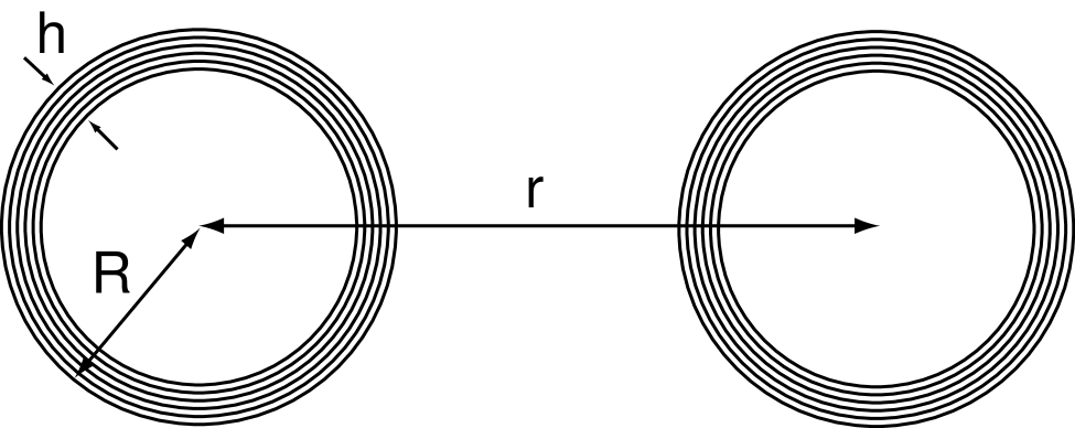
FIG. 1.: Schematic drawing of two multi-walled hollow nanoparticles with center-to-center distance $r$, particle radius $R$ and wall thickness $h$.

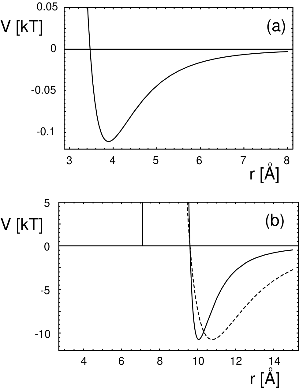
FIG. 2.: Different van der Waals interaction potentials: the Lennard-Jones potential for carbon atoms (a) is two orders of magnitude weaker than the Girifalco potential for buckyballs (b, solid). A Lennard-Jones potential with the same zero-crossing and potential depth as the Girifalco potential (b, dashed) shows that the Girifalco potential is rather short-ranged. The vertical line indicates that the potential diverges at a finite value of separation.

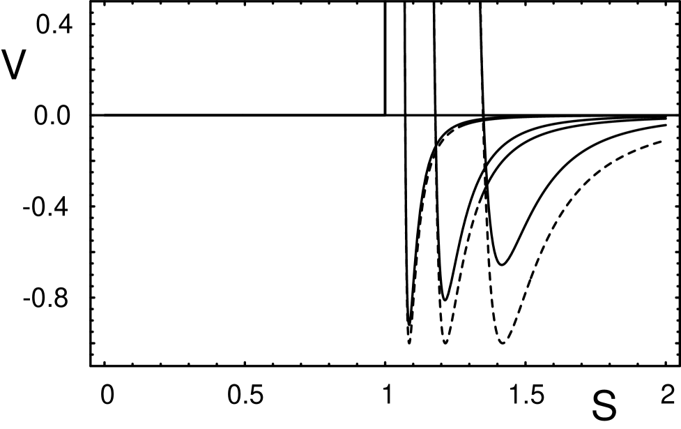
FIG. 3.: Interaction potential for single-walled nanoparticles: Girifalco potential (full) and Derjaguin approximation (dashed) for different values of $\eta=2R/\sigma$: from right to left $\eta=2.05$ (buckyballs), $4$ and $10$. All potentials are scaled such that the Derjaguin approximation has its minimum at $-1$. With increasing $\eta$, the potential well of the full potential falls into the range described by the Derjaguin approximation.

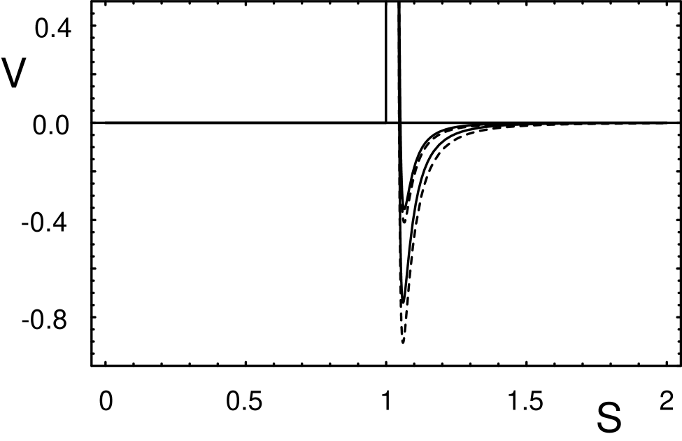
FIG. 4.: Interaction potential for multi-walled nanoparticles: Full potential (solid) and Derjaguin approximation (dashed) for $\eta=2R/\sigma=10$ and $\nu=h/\sigma=0.8$ (lower curves) and $0.4$ (upper curves). All potentials are scaled with the same factor as in Fig. 3. The Derjaguin approximation improves with increasing wall thickness $\nu$.

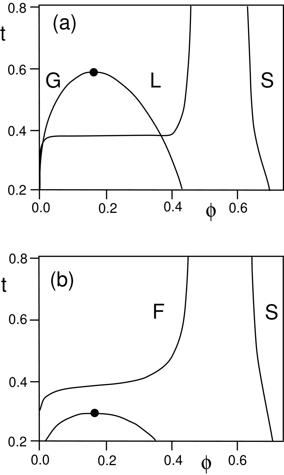
FIG. 5.: Phase diagrams (a) with and (b) without gas-liquid coexistence as a function of reduced temperature $t=kT/\epsilon$ and volume fraction $\phi=\pi\rho\sigma^{3}/6$. G, L, S and F denote gaseous, liquid, solid and fluid phases, respectively. In (b) the attractive interaction potential is so short-ranged that the gas-liquid coexistence (although existing by itself) is suppressed in the overall phase diagram by the fluid-solid coexistence. For a Double-Yukawa potential, the crossover between the two topologies of the phase diagram occurs when the interaction range decreases below the critical value $\delta\approx 0.4$.

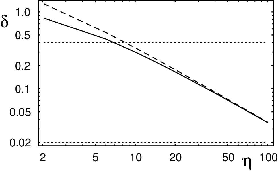
FIG. 6.: Double logarithmic plot of the interaction range $\delta$ of single-walled nanoparticles as a function of $\eta=2R/\sigma$ for the Girifalco potential (full) and its Derjaguin approximation (dashed). The dotted lines at $\delta=0.4$ and $\delta=0.02$ separate the long-, intermediate- and short-ranged regimes. Buckyballs with $\eta=2.05$ still have the gas-liquid coexistence which disappears only for $\delta<0.4$, that is $\eta>7$ ($R>12\ \AA$).

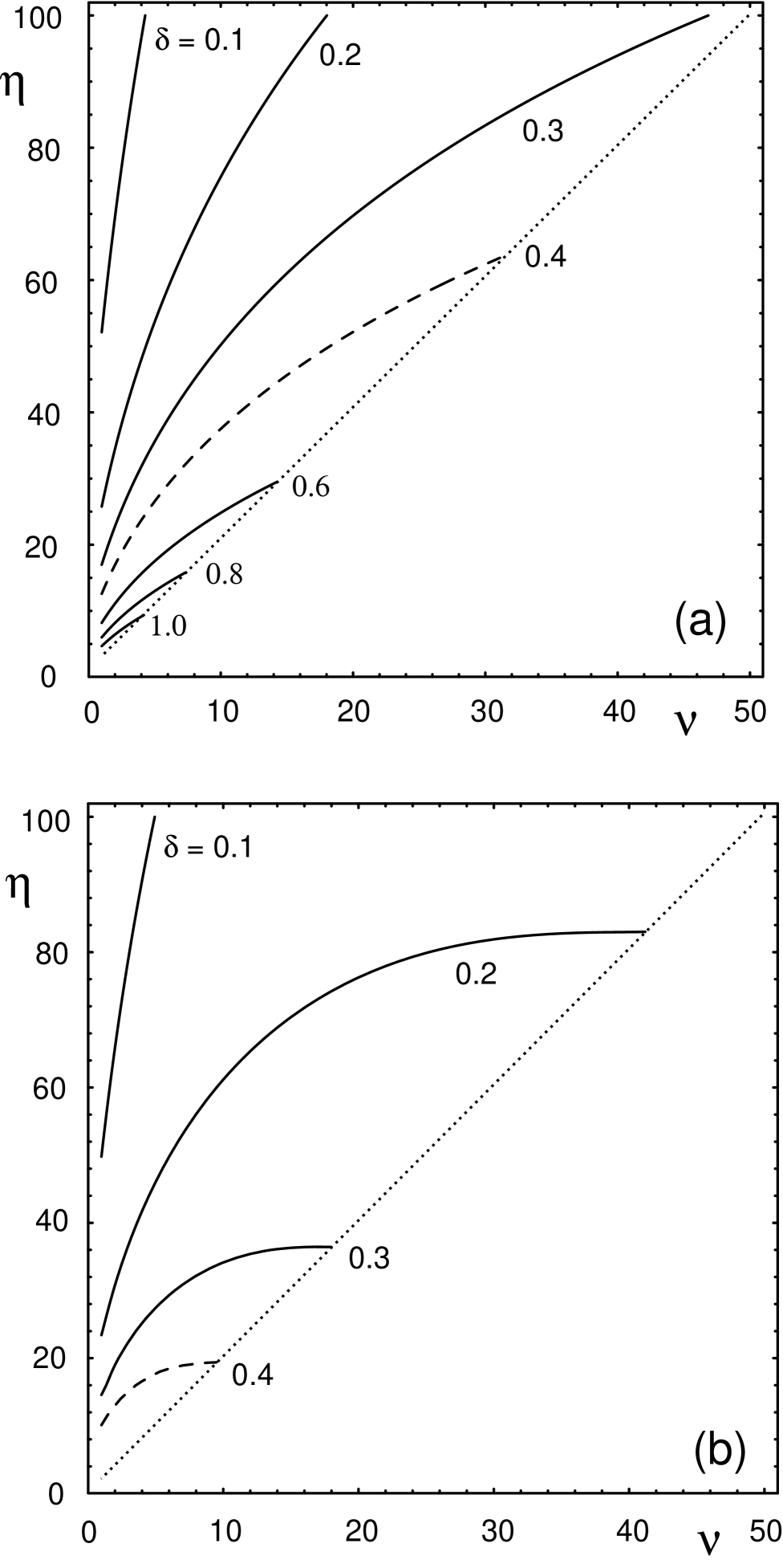
FIG. 7.: Interaction range $\delta$ of multi-walled nanoparticles as a function of $\eta=2R/\sigma$ and $\nu=h/\sigma$ for (a) Derjaguin approximation and (b) full potential. The dotted line delimits the allowed region $h\leq R$, that is $\eta\geq 2\nu$. The dashed line marks $\delta=0.4$. Only the region between the dotted and the dashed lines has a gas-liquid coexistence, whose size is overestimated in the Derjaguin approximation. Filled nanoparticles ($\eta=2\nu$) do not have a liquid phase for $\eta>20$ ($R>35\ \AA$).

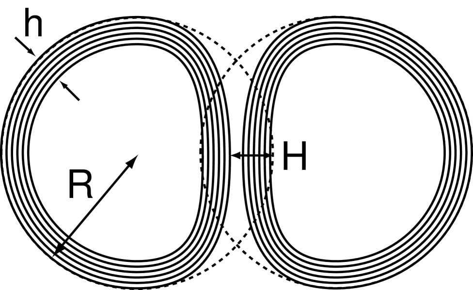
FIG. 8.: Schematic drawing of two multi-walled hollow nanoparticles deformed due to vdW adhesion. $H$ is the indentation. It follows geometrically that the contact area scales with $RH$.

REFERENCES

- [1] J. P. Hansen and I. R. McDonald, Theory of simple liquids (Academic Press, London, 1986).
- [2] W. B. Russel, D. A. Saville, and W. R. Schowalter, Colloidal dispersions (Cambridge University Press, Cambridge, 1989).
- [3] A. P. Gast, C. K. Hall, and W. B. Russel, J. Coll. Inter. Sci. 96, 251 (1983).
- [4] J. S. Huang et al., Phys. Rev. Lett. 53, 592 (1984).
- [5] P. Bolhuis and D. Frenkel, Phys. Rev. Lett. 72, 2211 (1994); P. Bolhuis, M. Hagen, and D. Frenkel, Phys. Rev. E 50, 4880 (1994).
- [6] A. Daanoun, C. F. Tejero, and M. Baus, Phys. Rev. E 50, 2913 (1994); T. Coussaert and M. Baus, Phys. Rev. E 52, 862 (1995).
- [7] C. F. Tejero, A. Daanoun, H. N. W. Lekkerkerker, and M. Baus, Phys. Rev. Lett. 73, 752 (1994); Phys. Rev. E 51, 558 (1995).
- [8] L. A. Girifalco, J. Phys. Chem. 96, 858 (1992).
- [9] P. A. Heiney et al., Phys. Rev. Lett. 66, 2911 (1991).
- [10] A. Cheng, M. L. Klein, and C. Caccamo, Phys. Rev. Lett. 71, 1200 (1993).
- [11] M. H. J. Hagen et al., Nature 365, 425 (1993).
- [12] C. Caccamo, D. Costa, and A. Fucile, J. Chem. Phys. 106, 255 (1997).
- [13] M. Hasegawa and K. Ohno, J. Chem. Phys. 111, 5955 (1999).
- [14] R. Tenne, Adv. Mater. 7, 965 (1995); review to appear in Progress in Inorg. Chem.
- [15] D. Ugarte, Nature 359, 707 (1992); Europhys. Lett. 22, 45 (1993).
- [16] R. Tenne, L. Margulis, M. Genut, and G. Hodes, Nature 360, 444 (1992); L. Margulis, G. Salitra, R. Tenne, and M. Talianker, Nature 365, 113 (1993); Y. Feldman, E. Wasserman, D. J. Srolovitz, and R. Tenne, Science 267, 222 (1995).
- [17] E. Donath et al., Angew. Chem. Int. Ed. 37, 2202 (1998).
- [18] F. Caruso, R. A. Caruso, and H. Möhwald, Science 282, 1111 (1998).
- [19] C. J. Smith, N. Grigorieff, and B. M. F. Pearse, EMBO J. 17, 4943 (1998).
- [20] J. Mahanty and B. W. Ninham, Dispersion Forces (Academic Press, London, 1976).
- [21] J. N. Israelachvili, Intermolecular and surface forces (Academic Press, London, 1992).
- [22] S. A. Safran, Statistical thermodynamics of surfaces, interfaces, and membranes, Vol. 90 of Frontiers in Physics (Addison-Wesley, Reading, 1994).
- [23] L. A. Girifalco and R. A. Lad, J. Chem. Phys. 25, 693 (1956).
- [24] C. Pan et al., J. Phys. Chem. 95, 2944 (1991).
- [25] J. E. Fischer et al., Science 252, 1288 (1991).
- [26] N. W. Ashcroft and N. D. Mermin, Solid State Physics (Saunders College, Philadelphia, 1976).
- [27] H. Guerin, J. Phys.: Condens. Matter 10, L527 (1998).
- [28] R. S. Ruoff et al., Nature 364, 514 (1993); J. Tersoff and R. S. Ruoff, Phys. Rev. Lett. 73, 676 (1994); T. Hertel, R. E. Walkup, and P. Avouris, Phys. Rev. B 58, 13870 (1998).
- [29] U. S. Schwarz, S. Komura, and S. A. Safran, Europhys. Lett. 50, 762 (2000).
- [30] L. D. Landau and E. M. Lifshitz, Theory of elasticity, Vol. 7 of Course of Theoretical Physics, 2nd ed. (Pergamon Press, Oxford, 1970).
- [31] D. J. Srolovitz, S. A. Safran, and R. Tenne, Phys. Rev. E 49, 5260 (1994).
- [32] Landolt and Börnstein, Units and fundamental constants in physics and chemistry (Springer, Berlin, 1991).