Damped Bogoliubov excitations of a condensate interacting with a static thermal cloud

Abstract

We calculate the damping of condensate collective excitations at finite temperatures arising from the lack of equilibrium between the condensate and thermal atoms. Since a static thermal cloud already produces damping in our model, we ignore the non-condensate dynamics. We derive a set of generalized Bogoliubov equations for finite temperatures that contain an explicit damping term due to collisional exchange of atoms between the two components. We have numerically solved these Bogoliubov equations to obtain the temperature dependence of the damping of the condensate modes in a harmonic trap. We compare these results with our recent work based on the Thomas-Fermi approximation.

I Introduction

In this paper, we calculate the damping at finite temperatures of collisionless condensate collective modes due to interactions with a static thermal cloud. Our treatment starts with the general theory developed in Ref. Zaremba99 and is an extension of the static Hartree-Fock-Bogoliubov Popov (HFB-Popov) approximation Hutchinson97 ; Dodd98 ; Dodd98b to include the effect of the lack of diffusive equilibrium between the condensate and non-condensate. The static thermal cloud acts as a reservoir that can exchange particles with the condensate so as to bring the condensate back into equilibrium, resulting in a damping of the collective oscillations of the condensate. We do not expect, in general, that the collisional damping we find from a static thermal cloud will be much modified when we treat the non-condensate dynamically. Because we are treating the non-condensate statically, Landau and Beliaev damping are not contained within in our description.

Our present work is the natural extension of a recent study Williams2000 of the damping of collisionless condensate collective modes at finite temperatures. This was based on a simplified model treating the time-dependent Gross-Pitaevskii equation for the condensate within the Thomas-Fermi approximation (TFA). We described the damping in terms of the density $\delta n_{c}({\bf r},t)$ and velocity $\delta{\bf v}_{c}({\bf r},t)$ fluctuations of the condensate oscillations. At $T=0$, where the non-condensate component is absent, Stringari Stringari96 showed that a simple analytic solution of the condensate collective modes could be obtained within the Thomas-Fermi approximation. In Ref. Williams2000 , we formally generalized these “Stringari” solutions to finite temperatures by assuming that the mean field of the static thermal cloud has a negligible effect on the condensate oscillations. We then calculated the damping due to the lack of equilibrium between the condensate and non-condensate to first order in perturbation theory, using the Stringari modes as a zeroth-order solution. In Ref. Williams2000 we compared this damping directly to Landau damping and found it gives a $30\%$ to $50\%$ correction to the total damping for typical experimental parameters.

The main focus of the present paper is to generalize our earlier work Williams2000 to include the same inter-component collisional damping mechanism directly in the Bogoliubov equations, still treating the non-condensate statically. This allows us to check the range of validity of the TFA made in Ref. Williams2000 . The TFA is valid when the number of condensate atoms $N_{c}$ is large, that is, when the condensate radius $R_{\rm{TF}}$ is much larger than the harmonic oscillator length $r_{\rm{HO}}$ Dalfovo99

$$r_{\rm{HO}}/R_{\rm{TF}}=(15N_{c}a/r_{\rm{HO}})^{-1/5}\ll 1,$$ (1)

where $a$ is the $s$-wave scattering length. The TFA will break down as one approaches the BEC transition temperature $T_{\rm{BEC}}$ where $N_{c}$ becomes small. It is in this temperature region where we must solve the coupled Bogoliubov equations for our model, as we do in this paper. From the time-dependent GP equation describing the fluctuations of the condensate order parameter, $\delta\Phi({\bf r},t)$, we derive generalized Bogoliubov equations for the collective mode amplitudes $u_{j}({\bf r})$ and $v_{j}({\bf r})$ and complex energies $\varepsilon_{j}$, which we solve numerically and compare to the predictions of our earlier TFA calculation Williams2000 . We also give a careful discussion of the formal properties of coupled Bogoliubov equations which include damping, since this may be of more general interest than our specific model calculation.

II Static Popov approximation

Our starting point is the finite $T$ generalized GP equation derived in Ref. Zaremba99 (see also Refs. Stoof99 ; Walser99 .)

$$i\hbar{\partial\Phi({\bf r},t)\over\partial t} = \Big{[}-{\hbar^{2}\over 2m}\nabla^{2}+U_{\rm{ext}}({\bf r})+gn_{c}({\bf r},t)+2g\tilde{n}({\bf r},t)$$ (2)

$$- iR({\bf r},t)\Big{]}\Phi({\bf r},t),$$

where the interaction parameter $g=4\pi\hbar^{2}a/m$, $a$ is the $s$-wave scattering length, $n_{c}({\bf r},t)=|\Phi({\bf r},t)|^{2}$, and $\tilde{n}({\bf r},t)=\int d{\bf p}f({\bf p},{\bf r},t)/(2\pi\hbar)^{3}$ is the non-condensate local density. The term $R({\bf r},t)$ in (2) describes the exchange of atoms between the condensate and normal gas and is given by

$$R({\bf r},t)={\hbar\over{2n_{c}({\bf r},t)}}\int{d{\bf p}\over(2\pi\hbar)^{3}}C_{12}[f({\bf p},{\bf r},t),\Phi({\bf r},t)].$$ (3)

This involves the collision integral $C_{12}[f,\Phi]$ describing collisions of condensate atoms with the thermal atoms, which also enters the approximate semi-classical kinetic equation for the single-particle distribution function (valid for $k_{\rm{B}}T\gg\mu_{c0}$) Zaremba99

$${\partial f({\bf p},{\bf r},t)\over\partial t} + {{\bf p}\over m}\cdot\nabla_{\bf r}f({\bf p},{\bf r},t)-\nabla U({\bf r})\cdot\nabla_{{\bf p}}f({\bf p},{\bf r},t)$$ (4)

$$= C_{12}[f,\Phi]+C_{22}[f]\,.$$

Here the collision integral denoted by $C_{22}[f]$ describes binary collisions between non-condensate atoms. It does not change the number of condensate atoms and hence does not appear explicitly in the GP equation (2). These coupled equations (2)-(4) (along with expressions (LABEL:eqa1) and (58) in Appendix A for the collision integrals $C_{12}$ and $C_{22}$) were derived in the semi-classical approximation. They assume that the atoms in the thermal cloud are well-described by the single-particle Hartree-Fock spectrum $\tilde{\varepsilon}_{p}({\bf r},t)=p^{2}/2m+U({\bf r},t)$, where $U({\bf r},t)=U_{\rm ext}({\bf r})+2g[n_{c}({\bf r},t)+\tilde{n}({\bf r},t)]$. However, they are expected to contain the essential physics in trapped Bose-condensed gases at finite $T$, in both the collisionless and hydrodynamic domains.

If the gas is weakly disturbed from equilibrium, one can consider linearized collective oscillations about equilibrium by writing

$$\Phi({\bf r},t) = e^{-i\mu_{c0}t/\hbar}\big{[}\Phi_{0}({\bf r})+\delta\Phi({\bf r},t)\big{]},$$ (5)

$$f({\bf p},{\bf r},t) = f^{0}({\bf p},{\bf r})+\delta f({\bf p},{\bf r},t).$$ (6)

Substituting (5) and (6) into Eqs. (2)-(4), one can obtain the coupled dynamical equations for the damped oscillations of the condensate $\delta\Phi({\bf r},t)$ and non-condensate $\delta f({\bf p},{\bf r},t)$. We find that the damping term $R({\bf r},t)$ in (3) is finite even if we only keep the equilibrium part of $f({\bf p},{\bf r},t)$. This approximation simplifies the problem tremendously and should give a good first estimate since $\delta f({\bf p},{\bf r},t)\ll f^{0}({\bf p},{\bf r})$.

The thermal cloud influences the dynamics of the condensate through two terms in (2), the mean-field interaction potential $2g\tilde{n}({\bf r},t)$ and the second-order collisional term $iR({\bf r},t)$. Let us first consider the effect of the term $2g\tilde{n}({\bf r},t)$. In the static approximation, the term $2g\tilde{n}_{0}({\bf r})$ gives rise to a temperature-dependent frequency shift of the condensate collective modes, but does not give rise to damping. Landau damping appears only when the dynamics of the non-condensate $\delta\tilde{n}({\bf r},t)$ is accounted for (i.e. when we keep $\delta f({\bf p},{\bf r},t)$). An important point is that the collisional damping described by the second-order term $iR({\bf r},t)$ in (2) arises already within the static approximation $\delta f({\bf p},{\bf r},t)=0$, in contrast to Landau damping.

The damped collective mode equations for the condensate can be obtained if we substitute the equilibrium distribution $f^{0}({\bf p},{\bf r})$ and density $\tilde{n}_{0}({\bf r})$ of the non-condensate into (2), giving us

$$i\hbar{\partial\Phi({\bf r},t)\over\partial t} = \Big{[}-{\hbar^{2}\over 2m}\nabla^{2}+U_{\rm{ext}}({\bf r})+gn_{c}({\bf r},t)+2g\tilde{n}_{0}({\bf r})$$ (7)

$$- iR_{0}({\bf r},t)\Big{]}\Phi({\bf r},t),$$

which describes the condensate motion coupled to the static thermal cloud. Here the damping term $R_{0}({\bf r},t)$ is

$$R_{0}({\bf r},t)\equiv{\hbar\over{2n_{c}({\bf r},t)}}\int{d{\bf p}\over(2\pi\hbar)^{3}}C_{12}[f^{0}({\bf p},{\bf r}),\Phi({\bf r},t)].$$ (8)

Notice that $R_{0}({\bf r},t)$ now depends on time only through $\Phi({\bf r},t)$, which has to be determined self-consistently by solving (7).

The equilibrium stationary solution of the coupled equations (2)-(4) is given by the solution of the generalized time-independent Gross-Pitaevskii equation

$$\hat{H}_{0}\Phi_{0}({\bf r})=\mu_{c0}\Phi_{0}({\bf r}),$$ (9)

where we have defined the Hermitian operator

$$\hat{H}_{0}=-{\hbar^{2}\over 2m}\nabla^{2}+U_{\rm{ext}}({\bf r})+gn_{c0}({\bf r})+2g\tilde{n}_{0}({\bf r}).$$ (10)

Here, $n_{c0}({\bf r})=|\Phi_{0}({\bf r})|^{2}$ is the static equilibrium density of the condensate and $\tilde{n}_{0}({\bf r})$ is the equilibrium density of the non-condensate. The equilibrium chemical potential of the condensate $\mu_{c0}$ is independent of position and can be written explicitly in terms of the equilibrium densities as

$$\mu_{c0}=-{\hbar^{2}{\nabla}^{2}\sqrt{n_{c0}({\bf r})}\over 2m\sqrt{n_{c0}({\bf r})}}+U_{\rm ext}({\bf r})+gn_{c0}({\bf r})+2g\tilde{n}_{0}({\bf r}),$$ (11)

where the first term on the right-hand side of (11) is the so-called quantum pressure of the static condensate wave function.

To be consistent with the underlying kinetic model developed in Ref. Zaremba99 , the static thermal cloud is described using the single-particle HF spectrum (see above). Thus the equilibrium distribution $f^{0}({\bf p},{\bf r})$ of the non-condensate atoms is given by the Bose-Einstein distribution

$$f^{0}({\bf p},{\bf r})={1\over{e^{\beta[p^{2}/2m+U_{0}({\bf r})-\tilde{\mu}_{0}]}-1}}\,,$$ (12)

where $\beta=1/k_{B}T$, $\tilde{\mu}_{0}$ is the equilibrium chemical potential of the non-condensate, and $U_{0}({\bf r})=U_{\rm{ext}}({\bf r})+2g[n_{c0}({\bf r})+\tilde{n}_{0}({\bf r})]$. As discussed in Ref. Zaremba99 , the static chemical potentials of the two components are equal ($\tilde{\mu}_{0}=\mu_{c0}$) in equilibrium.

The equilibrium density of the non-condensate $\tilde{n}_{0}({\bf r})$ is obtained by integrating (12) over momentum to give the usual result

$$\tilde{n}_{0}({\bf r})={1\over{\Lambda^{3}}}g_{3/2}[z_{0}({\bf r})].$$ (13)

Here, $\Lambda=(2\pi\hbar^{2}\beta/m)^{1/2}$ is the thermal de Broglie wavelength and $g_{3/2}(z)$ is a Bose-Einstein function. The local fugacity is $z_{0}({\bf r})=e^{\beta(\tilde{\mu}_{0}-U_{0}({\bf r}))}$.

We recall that in the TF approximation used in our earlier work Williams2000 , (11) reduces to $\mu_{c0}=U_{\rm{ext}}+gn_{c0}+2g\tilde{n}_{0}$ and hence $z_{0}({\bf r})=e^{-\beta gn_{c0}({\bf r})}$. When we keep the quantum pressure terms in (11), the analysis is more complicated. The equilibrium solutions for the condensate and thermal cloud, given by (9) and (12), must be obtained self-consistently. For completeness, we outline our procedure for a given value of the temperature $T$ and with the total number of atoms $N$ fixed (see also Ref. Giorgini97 ):

1. For a given value of the condensate population $N_{c}\leq N$, the equilibrium solution of the condensate is obtained by solving (9) numerically Williams99 . To start the procedure, we initially take $\tilde{n}_{0}=0$.

2. Using $\mu_{c0}$ and $n_{c0}({\bf r})=|\Phi_{0}({\bf r})|^{2}$ found from step 1, the non-condensate density $\tilde{n}_{0}({\bf r})$ is obtained from (13), using $\tilde{\mu}_{0}=\mu_{c0}$. If $\mu_{c0}>{\rm{min}}\big{\{}U({\bf r})\big{\}}$, which can occur for small condensates at temperatures close to $T_{\rm{BEC}}$, we set $\tilde{\mu}_{0}={\rm{min}}\big{\{}U({\bf r})\big{\}}$.

3. Steps 1 and 2 are repeated until convergence is reached to the desired accuracy (in our calculations, when $\mu_{c0}$ stops varying up to an error of $10^{-5}$).

4. The number of atoms in the thermal cloud is calculated $\tilde{N}=\int d{\bf r}\tilde{n}_{0}({\bf r})$. We then repeat steps 1 - 3, varying $N_{c}$ until the chosen total number of atoms, $N=N_{c}+\tilde{N}$, is obtained to the desired accuracy (in our calculations, we obtain $N$ to an error of less than $10^{-4}$).

The equilibrium values of $n_{c0}({\bf r})$, $\mu_{c0}=\tilde{\mu}_{0}$, and $\tilde{n}_{0}({\bf r})$ obtained from the above procedure are used in the calculation of the damped collective oscillations of the condensate discussed in the next section.

Before proceeding, though, it is useful to emphasize several points about our approximate model, as described by (7) and (8). Our emphasis in this paper, and the earlier TF version in Ref. Williams2000 , is on the calculation of damping due to collisional exchange of atoms between a dynamic condensate and a static thermal cloud. While we use the semi-classical HF excitations to calculate $f^{0}({\bf p},{\bf r})$, which leads to (11) and (12), we do not expect improved treatments of the static thermal cloud will greatly alter our estimates of the inter-component condensate damping we are considering. There is a considerable literature on the calculation of the undamped condensate mode frequencies at finite $T$. One finds that the frequency shifts are quite dependent on the specific approximation Hutchinson97 ; Dodd98 ; Dodd98b used for the non-condensate mean field $2g\tilde{n}_{0}({\bf r})$, as well as on other terms left out of (7) related to the anomalous correlation function $\tilde{m}_{0}({\bf r})=\langle\tilde{\psi}({\bf r})\tilde{\psi}({\bf r})\rangle$ We are not concerned with these questions here, but refer to Refs. Giorgini2000 ; Bergeman2000 for further studies.

III Bogoliubov equations with damping

Using the explicit general expression for $C_{12}$ given in (58) of Appendix A, it was shown in Ref. Zaremba99 that $R_{0}({\bf r},t)$ can be simplified to (see also Ref. Gardiner2000 )

$$R_{0}({\bf r},t)={\hbar\over{2\tau_{12}({\bf r},t)}}\big{[}e^{-\beta(\tilde{\mu}_{0}-\varepsilon_{c}({\bf r},t))}-1\big{]},$$ (14)

where we have defined the relaxation rate due to inter-component $C_{12}$ collisions

$${1\over{\tau_{12}({\bf r},t)}} \equiv {2g^{2}\over(2\pi)^{5}\hbar^{7}}\!\int\!\!d{\bf p}_{1}\!\int\!\!d{\bf p}_{2}\!\int\!\!d{\bf p}_{3}\delta({\bf p}_{c}+{\bf p}_{1}-{\bf p}_{2}-{\bf p}_{3})$$ (15)

$$\times \delta(\varepsilon_{c}+\tilde{\varepsilon}_{p_{1}}-\tilde{\varepsilon}_{p_{2}}-\tilde{\varepsilon}_{p_{3}})(1+f_{1}^{0})f_{2}^{0}f_{3}^{0}\,.$$

The condensate atom local energy is $\varepsilon_{c}({\bf r},t)=\mu_{c}({\bf r},t)+{1\over 2}mv_{c}^{2}({\bf r},t)$ with the non-equilibrium condensate chemical potential

$$\mu_{c}({\bf r},t)=-{\hbar^{2}{\nabla}^{2}\sqrt{n_{c}({\bf r},t)}\over 2m\sqrt{n_{c}({\bf r},t)}}+U_{\rm ext}({\bf r})+gn_{c}({\bf r},t)+2g\tilde{n}_{0}({\bf r})\,.$$ (16)

The condensate atom momentum is ${\bf p}_{c}=m{\bf v}_{c}$, and $f_{i}^{0}=f^{0}({\bf r},{\bf p}_{i})$. We have introduced the usual condensate velocity defined in terms of the phase $\theta$ of the condensate $\Phi({\bf r},t)=\sqrt{n_{c}({\bf r},t)}e^{i\theta({\bf r},t)}$ as ${\bf v}_{c}=\hbar{\nabla}\theta({\bf r},t)/m$. A closed set of equations for $\Phi({\bf r},t)$ is given by (7) combined with (12) and (14) - (16). The damping term $R_{0}({\bf r},t)$ given in (14) vanishes when the condensate is in diffusive equilibrium with the thermal cloud, when $\varepsilon_{c}({\bf r},t)=\mu_{c0}=\tilde{\mu}_{0}$.

We obtain the linearized equation of motion for the condensate fluctuation $\delta\Phi({\bf r},t)$ by expanding all condensate variables appearing in (7) to first order in $\delta\Phi({\bf r},t)$. For simplicity we assume $\Phi_{0}({\bf r})$ is real, that is, ${\bf v}_{c0}({\bf r})=0$. Using (5), the condensate density $n_{c}({\bf r},t)=|\Phi_{0}({\bf r})+\delta\Phi({\bf r},t)|^{2}$ can be written $n_{c}({\bf r},t)=n_{c0}({\bf r})+\delta n_{c}({\bf r},t)$, where the linearized density fluctuation of the condensate is

$$\delta n_{c}({\bf r},t)=\Phi_{0}({\bf r})\big{[}\delta\Phi({\bf r},t)+\delta\Phi^{*}({\bf r})\big{]}.$$ (17)

We can also simplify $R_{0}({\bf r},t)$ in (14) by noting that, to first order in the condensate fluctuations, we can write $\varepsilon_{c}({\bf r},t)=\mu_{c}({\bf r},t)$ (neglecting the quadratic term $(\delta v_{c})^{2}$). Using (11), the condensate chemical potential (16) can be written as

$$\mu_{c}({\bf r},t)=\mu_{c0}+\delta\mu_{c}({\bf r},t),$$ (18)

where the linearized fluctuation in the local condensate chemical potential is found to be given by

$$\delta\mu_{c}({\bf r},t)={1\over{2\Phi_{0}}}(\hat{H}_{0}-\mu_{c0})\Big{[}{\delta n_{c}({\bf r},t)\over\Phi_{0}({\bf r})}\Big{]}+g\delta n_{c}({\bf r},t).$$ (19)

where the operator $\hat{H}_{0}$ is defined in (10). The first term in (19) arises from the dynamic quantum pressure of the condensate oscillation, while the second term comes from the mean field interaction. The latter is the only contribution kept in the TF approximation used in Ref. Williams2000 . Note that because the non-condensate is static, there is no contribution in (19) from the fluctuation in the HF mean field ($2g\,\delta\tilde{n}$) of the thermal cloud.

Utilizing the fact that $\mu_{c0}=\tilde{\mu}_{0}$ in static equilibrium, $R_{0}({\bf r},t)$ in (14) can be simplified to

$$\delta R_{0}({\bf r},t)={\hbar\beta\over{2\tau_{12}^{0}({\bf r})}}\delta\mu_{c}({\bf r},t)\,,$$ (20)

where the “equilibrium” $C_{12}$ collision rate is defined by (compare with (15))

$${1\over{\tau^{0}_{12}({\bf r})}} \equiv {2g^{2}\over(2\pi)^{5}\hbar^{7}}\int d{\bf p}_{1}\int d{\bf p}_{2}\int d{\bf p}_{3}\delta({\bf p}_{1}-{\bf p}_{2}-{\bf p}_{3})$$ (21)

$$\times \delta\big{(}{p_{1}^{2}-p_{2}^{2}-p_{3}^{2}\over{2m}}-gn_{c0}\big{)}(1+f_{1}^{0})f_{2}^{0}f_{3}^{0}\,.$$

We can now obtain an equation of motion for the condensate fluctuation $\delta\Phi({\bf r},t)$ by substituting (5) into (7) and using the above results

$$i\hbar{\partial\delta\Phi({\bf r},t)\over{\partial t}} = \hat{\cal L}\,\delta\Phi({\bf r},t)+gn_{c0}({\bf r})\delta\Phi^{*}({\bf r},t)$$ (22)

$$- i\hat{\Gamma}\,\big{[}\delta\Phi({\bf r},t)+\delta\Phi^{*}({\bf r},t)\big{]},$$

We find it convenient to define the operators $\hat{\cal L}=\hat{H}_{0}+gn_{c0}-\mu_{c0}$ and

$$\hat{\Gamma}={\hbar\beta\over{2\tau_{12}^{0}}}\Big{[}\frac{1}{2}\big{(}\hat{H}_{0}-\mu_{c0}\big{)}+gn_{c0}\Big{]},$$ (23)

both of which are Hermitian. The first term in (23) arises from the quantum pressure of the condensate fluctuation. It is neglected in the Thomas-Fermi approximation, valid in the large $N_{c}$ limit. The damping operator can also be written in an alternative form as $\hat{\Gamma}=(\hbar\beta/4\tau_{12}^{0})[\hat{\cal L}+gn_{c0}({\bf r})]$.

We now consider normal mode oscillations of the condensate by expanding $\delta\Phi({\bf r},t)$ as

$$\delta\Phi({\bf r},t)=u_{j}({\bf r})e^{-i\varepsilon_{j}t/\hbar}+v_{j}^{*}({\bf r})e^{i\varepsilon_{j}^{*}t/\hbar},$$ (24)

where the excitation energy $\varepsilon_{j}$ and the collective mode amplitudes $u_{j}({\bf r})$ and $v_{j}({\bf r})$, in general, have real and imaginary components. Substituting this into (22) and equating like powers of $e^{\pm i\varepsilon_{j}t/\hbar}$, we obtain the damped finite-$T$ Bogoliubov equations

$$\big{(}\hat{\cal L}-i\hat{\Gamma}\big{)}u_{j}({\bf r})+\big{(}gn_{c0}-i\hat{\Gamma}\big{)}v_{j}({\bf r}) = \varepsilon_{j}u_{j}({\bf r})$$

$$\big{(}\hat{\cal L}+i\hat{\Gamma}\big{)}v_{j}({\bf r})+\big{(}gn_{c0}+i\hat{\Gamma}\big{)}u_{j}({\bf r}) = -\varepsilon_{j}v_{j}({\bf r}).$$ (25)

The real and imaginary parts of $\varepsilon_{j}$ give the oscillation frequency $\omega_{j}\equiv{\rm{Re}}\varepsilon_{j}/\hbar$ and the damping rate $\gamma_{j}\equiv-{\rm{Im}}\varepsilon_{j}/\hbar$, which vary with temperature $T$. These coupled equations are the main new result of this paper. They describe the damped collective modes of a condensate coupled to a static thermal cloud at finite $T$. It is important to realize that the anti-Hermitian operator $i\hat{\Gamma}$ appearing in (25) has not simply been inserted “by hand” based on phenomenological arguments, as is done in the theories developed in Refs. Pitaevskii59 ; Hutchinson99 ; Choi98 , but has been derived explicitly starting from a microscopic (albeit approximate) theory. The origin of this damping is the lack of collisional detailed balance between the condensate and non-condensate, which occurs when the system is disturbed from equilibrium. This mechanism is distinct from the Landau damping process, which arises from the mean field interaction between components when the dynamics $\delta f({\bf p},{\bf r},t)$ of the non-condensate is taken into account Giorgini2000 .

In order to explore the properties of the coupled Bogoliubov equations (25), it is useful to write it in matrix form

$$\hat{M}w_{j}=\varepsilon_{j}\sigma_{3}w_{j},$$ (26)

where $\hat{M}=\hat{M}_{0}+\hat{M}^{\prime}$ and

$$\begin{array}[]{ccc}\hat{M}_{0}&=&\left(\begin{array}[]{cc}\hat{\cal L}&gn_{c0}\\ gn_{c0}&\hat{\cal L}\end{array}\right),\end{array}$$ (27)

$$\begin{array}[]{ccc}\hat{M}^{\prime}&=&-i\hat{\Gamma}\left(\begin{array}[]{cc}1&1\\ -1&-1\end{array}\right),\end{array}$$ (28)

$$\begin{array}[]{ccc}\sigma_{3}&=&\left(\begin{array}[]{cc}1&0\\ 0&-1\end{array}\right),\end{array}$$ (29)

$$\begin{array}[]{ccc}w_{j}({\bf r})&=&\left(\begin{array}[]{c}u_{j}({\bf r})\\ v_{j}({\bf r})\end{array}\right).\end{array}$$ (30)

Since $\hat{M}^{\prime}$ is not a Hermitian operator, the solutions of (26) are not in general orthogonal to one another and the energies $\varepsilon_{j}$ are expected to have an imaginary component describing damping. We can see this explicitly by deriving a generalized orthogonality relation for the solutions $w_{j}$ Fetter72 ; Blaizot . Multiplying (26) on the left-hand side by $w_{i}^{\dagger}$ and integrating over position, we find

$$\int d{\bf r}w_{i}^{\dagger}({\bf r})\hat{M}w_{j}({\bf r})=\varepsilon_{j}\int d{\bf r}w_{i}^{\dagger}({\bf r})\sigma_{3}w_{j}({\bf r}).$$ (31)

Taking the Hermitian conjugate of (26), replacing the index $j$ by $i$, multiplying on the right-hand side by $w_{j}$, and integrating over position, we obtain

$$\int d{\bf r}w_{i}^{\dagger}({\bf r})\hat{M}^{\dagger}w_{j}({\bf r})=\varepsilon_{i}^{*}\int d{\bf r}w_{i}^{\dagger}({\bf r})\sigma_{3}w_{j}({\bf r}).$$ (32)

Subtracting (31) from (32) gives us the desired orthogonality relation

$$(\varepsilon_{i}^{*}-\varepsilon_{j})\int d{\bf r}w_{i}^{\dagger}({\bf r})\sigma_{3}w_{j}({\bf r})=2i\int d{\bf r}w_{i}^{\dagger}({\bf r})\sigma_{3}\hat{\Gamma}w_{j}({\bf r}).$$ (33)

where we have used the Hermitian property $\hat{M}_{0}=\hat{M}_{0}^{\dagger}$ and used the fact that $(\hat{M}^{\prime\dagger}-\hat{M}^{\prime})=2i\sigma_{3}\hat{\Gamma}$.

If we neglect the damping term $\hat{\Gamma}=0$ in (26), our description reduces to the usual coupled Bogoliubov equations at finite temperatures for the collective modes $u_{0j}({\bf r})$ and $v_{0j}({\bf r})$ in the static Popov approximation Hutchinson97 ; Dodd98 ; Dodd98b ; Griffin96

$$\hat{M}_{0}w_{0j}=\varepsilon_{0j}\sigma_{3}w_{0j}.$$ (34)

With $\hat{\Gamma}=0$ in (33), we see that these solutions $w_{0j}$ obey the orthogonality condition

$$(\varepsilon_{0i}^{*}-\varepsilon_{0j})\int d{\bf r}w_{0i}^{\dagger}\sigma_{3}w_{0j}=0.$$ (35)

It then follows that the eigenvalues must be real ($\varepsilon_{0j}=\varepsilon_{0j}^{*}$), otherwise the solution $w_{0j}$ of (34) would have zero norm . This property follows from the fact that $\hat{M}_{0}$ is a Hermitian operator. We note that at $T=0$, where $2g\tilde{n}_{0}=0$ in $\hat{M}_{0}$, (34) reduces to the standard Bogoliubov equations Fetter72 ; Blaizot . At finite temperatures, the simplest way of including the non-condensate is to use the temperature dependent condensate number $N_{c}(T)$ (but ignore the mean-field term $2g\tilde{n}_{0}({\bf r})$ in $\hat{H}_{0}$) Dodd98b . As discussed in Williams2000 , the condensate normal mode frequencies at finite $T$ are the same as at $T=0$ in the Thomas-Fermi limit Stringari96 , since the frequencies at $T=0$ do not depend on the value of $N_{c}$ in this limit. Another effect comes from the mean field $2g\tilde{n}_{0}$ due to the non-condensate, which gives rise to a temperature-dependent energy shift to the excitation frequencies Hutchinson97 ; Dodd98 . However, as discussed at the end of Section II, a proper estimate of the shifts in the condensate normal mode frequencies requires a better model.

According to (33), the inclusion of the anti-Hermitian damping operator $i\hat{\Gamma}$ in the normal mode equations introduces an explicit imaginary part in the eigenenergies $\varepsilon_{j}$, without requiring the solutions to have zero norm. However, these damped solutions $w_{i}$ are not required to be orthogonal. From (33), the imaginary part of $\varepsilon_{j}$ is given by

$${\rm{Im}}\varepsilon_{j}={{-\int d{\bf r}w_{j}^{\dagger}\sigma_{3}\hat{\Gamma}w_{j}}\over{\int d{\bf r}w_{j}^{\dagger}\sigma_{3}w_{j}}}.$$ (36)

If the operator $\hat{\Gamma}$ in (23) was a scalar position-independent constant $\hat{\Gamma}=\gamma$, we can take it out of the integral in (33), and in this case the orthogonality condition for $w_{j}$ is recovered,

$$(\varepsilon_{i}^{*}-\varepsilon_{j}-2i\gamma)\int d{\bf r}w_{i}^{\dagger}\sigma_{3}w_{j}=0.$$ (37)

This states that for $i=j$, the imaginary part of each of the excitation energies is ${\rm{Im}}\varepsilon_{j}=-\gamma$ (unless the norm of $w_{j}$ is zero). For $i\neq j$, (37) shows that the eigenmodes $w_{i}$ and $w_{j}$ are orthogonal as long as ${\rm{Re}}\varepsilon_{i}\neq{\rm{Re}}\varepsilon_{j}$.

Since the damping effect of $C_{12}$ collisions on the condensate oscillations is weak, we can treat the damping term $\hat{M}^{\prime}$ in (28) using first order perturbation theory. More precisely, we assume

$$\hbar\omega_{j}\gg\gamma_{j},$$ (38)

where $\gamma_{j}=-{\rm{Im}}\varepsilon_{j}$ is the damping rate due to $C_{12}$ collisions given by (36). Proceeding as usual in perturbation theory, we introduce a small expansion parameter

$$\hat{M}=\hat{M}_{0}+\lambda\hat{M}^{\prime},$$ (39)

and expand the energies and eigenmodes as

$$\varepsilon_{j} = \varepsilon_{0j}+\lambda\varepsilon_{1j}+\lambda^{2}\varepsilon_{2j}+\cdots$$ (40)

$$w_{i} = w_{0j}+\lambda w_{1j}+\lambda^{2}w_{2j}+\cdots.$$ (41)

Substituting (39) - (41) into (26) and equating like powers of $\lambda$, we obtain a hierarchy of equations. Note that since $\hat{M}^{\prime}$ is also radially symmetric, it does not break the $(2l+1)$-fold degeneracy of the magnetic sublevels. The zeroth order equation simply reproduces (34) for the undamped modes $w_{0j}$. The first order correction is obtained from

$$\big{(}\hat{M}_{0}-\varepsilon_{0j}\sigma_{3}\big{)}w_{1j}=\big{(}\varepsilon_{1j}\sigma_{3}-\hat{M}^{\prime}\big{)}w_{0j}.$$ (42)

If we multiply (42) on the left by $w_{0j}^{\dagger}$ and integrate over position, the left-hand side of (42) vanishes using (34). This leaves us with the following result for the perturbed energy shift,

$$\varepsilon_{1j}={\int d{\bf r}w_{0j}^{\dagger}\hat{M}^{\prime}w_{0j}\over{\int d{\bf r}w_{0j}^{\dagger}\sigma_{3}w_{0j}}}.$$ (43)

Taking the Hermitian conjugate of (42), multiplying on the right by $w_{0j}$ and integrating over position, we obtain the analogous expression for the complex conjugate $\varepsilon_{1j}^{*}$

$$\varepsilon_{1j}^{*}={\int d{\bf r}w_{0j}^{\dagger}\hat{M}^{\prime\dagger}w_{0j}\over{\int d{\bf r}w_{0j}^{\dagger}\sigma_{3}w_{0j}}}.$$ (44)

From (43) and (44), we can obtain the damping (to first order)

$$\gamma_{0j}=-{\rm{Im}}\varepsilon_{1j}={\int d{\bf r}w_{0j}^{\dagger}\sigma_{3}\hat{\Gamma}w_{0j}\over{\int d{\bf r}w_{0j}^{\dagger}\sigma_{3}w_{0j}}}.$$ (45)

Here we have used $(\hat{M}^{\prime\dagger}-\hat{M}^{\prime})=2i\sigma_{3}\hat{\Gamma}$. The result in (45) is consistent with expression (36), had we simply expanded (36) about $w_{0j}$. We can also obtain the real part of $\varepsilon_{1j}$ from (43) and (44) and we find that this vanishes (see Appendix B), i.e.

$${\rm{Re}}\varepsilon_{1j}=0.$$ (46)

In summary, first order perturbation theory gives

$$\varepsilon_{j}=\varepsilon_{0j}-i\gamma_{0j}.$$ (47)

Using these results, the expansion given in (24) for the condensate oscillations can be written in the more explicit form

$$\delta\Phi({\bf r},t)=e^{-\gamma_{0j}t/\hbar}\big{(}u_{0j}({\bf r})e^{-i\varepsilon_{0j}t/\hbar}+v_{0j}^{*}({\bf r})e^{i\varepsilon_{0j}t/\hbar}\big{)}.$$ (48)

Using expression (45) to calculate $\gamma_{0j}$, one can check that the criterion in (38) is well satisfied. The difference between the perturbative results and the exact numerical solution of (25) is always less than $1\,\%$ in our calculations.

The results of the present calculation can be compared to those in Ref. Williams2000 , where we used a simplified model to calculate the damping rates $\gamma_{j}$. We used the Thomas-Fermi approximation (neglecting the kinetic energy pressure in the solution of $\Phi_{0}$ and $\mu_{c0}$) and we also neglected the contribution $2g\tilde{n}_{0}$ to the mean field interaction. We also neglected the kinetic energy pressure in the solution of the normal modes, which allowed us to use the $T=0$ Stringari normal mode solutions Stringari96 as a basis with which to treat the effect of $\delta R_{0}$ to first order. The main result of Ref. Williams2000 was the expression for the damping rate

$$\gamma_{j}={\hbar\over 2}{\int d{\bf r}\,\delta n_{{\rm{S}}j}^{2}({\bf r})/\tau^{\prime}({\bf r})\over\int d{\bf r}\,\delta n_{{\rm{S}}j}^{2}({\bf r})}.$$ (49)

Here $\delta n_{{\rm{S}}j}({\bf r})$ is the density fluctuation associated with a Stringari normal mode Stringari96 ; Williams2000 at finite $T$ and $1/\tau^{\prime}=(gn_{c0}/k_{B}T)(1/\tau_{12}^{0})$, with $1/\tau_{12}^{0}$ given in (21). This damping rate is easy to evaluate since the equilibrium form for the condensate $\Phi_{0}({\bf r})$, as well as the Stringari normal modes $\delta n_{\rm{S}j}({\bf r})$, are both given by simple analytic functions.

The TF result (49) can, of course, be obtained directly from (45) by taking the Thomas-Fermi limit. In this limit, the first term in (23) for $\hat{\Gamma}$, which describes the quantum pressure of the oscillation, can be neglected. We are left with $\Gamma({\bf r})=\hbar/2\tau^{\prime}({\bf r})$, and hence (45) reduces to

$$\gamma_{0j}={\hbar\over 2}{\int d{\bf r}w_{0j}^{\dagger}\sigma_{3}w_{0j}/\tau^{\prime}({\bf r})\over{\int d{\bf r}w_{0j}^{\dagger}\sigma_{3}w_{0}}}.$$ (50)

In Ref. Fetter98 , the product $w_{0j}^{\dagger}({\bf r})\sigma_{3}w_{0j}({\bf r})=|u_{j}({\bf r})|^{2}-|v_{j}({\bf r})|^{2}$ is shown to satisfy the following relationship

$$|u_{j}({\bf r})|^{2}-|v_{j}({\bf r})|^{2}={\rm{Re}}{-2im\over\hbar}\delta\phi_{j}^{*}({\bf r})\delta n_{j}({\bf r}),$$ (51)

where $\delta n_{j}({\bf r})$ is the density fluctuation of mode $j$, and $\delta\phi_{j}({\bf r})$ is the corresponding fluctuation in the velocity potential. In the Thomas-Fermi limit, the finite $T$ fluctuations in the density and velocity potential still have the simple relationship Wu96

$$\delta\phi_{{\rm{S}}j}({\bf r})={-ig\over{m\omega_{{\rm{S}}j}}}\delta n_{{\rm{S}}j}({\bf r}),$$ (52)

where $\omega_{{\rm{S}}j}$ is the Stringari frequency of mode $j$. Putting these results together, we have

$$w_{0j}^{\dagger}({\bf r})\sigma_{3}w_{0j}({\bf r})={2g\over{\hbar\omega_{j}}}\delta n_{{\rm{S}}j}^{2}({\bf r})$$ (53)

and hence (50) reduces to (49).

In the next section, we compare the damping given by (49) to the result given by (45) for a trapped gas. It is useful to apply (45) to the case of a homogeneous gas, where the modes are $u_{\bf k}({\bf r})=u_{k}e^{i{\bf k}\cdot{\bf r}}$ and $v_{\bf k}({\bf r})=v_{k}e^{i{\bf k}\cdot{\bf r}}$ and the energies are given by the usual Bogoliubov expression

$$\varepsilon_{k}=\sqrt{\Big{(}{\hbar^{2}k^{2}\over{2m}}\Big{)}\Big{(}{\hbar^{2}k^{2}\over{2m}}+2gn_{c0}\Big{)}}.$$ (54)

Using the expression for $\hat{\Gamma}$ given in (23), the damping rate (45) reduces to

$$\gamma_{k}={\hbar\beta\over{2\tau_{12}^{0}}}\Big{[}{\hbar^{2}k^{2}\over{4m}}+gn_{c0}\Big{]},$$ (55)

where $\tau_{12}^{0}$, as given in (21), is independent of position for a uniform Bose gas. The first term proportional to $k^{2}$ comes from the quantum pressure (i.e. the first term in (23)), which is omitted in the Thomas-Fermi result given in Ref. Williams2000 .

IV Numerical Results

We now turn to an explicit calculation of the inter-component damping of collective modes for a dilute Bose gas in a spherical harmonic trap $U_{\rm{ext}}({\bf r})=\frac{1}{2}m\omega_{0}^{2}r^{2}$. We choose the same set of physical parameters as given in Ref. Williams2000 : the frequency of the trap is $\omega_{0}/{2\pi}=10$ Hz, the scattering length for ⁸⁷Rb is $a=5.7$ nm, and the total number of atoms is $N=2\times 10^{6}$.

IV.1 Equilibrium solution

In Fig. 1 we plot the condensate fraction versus temperature for the case of $N=2\times 10^{6}$ atoms. The solid line corresponds to the full calculation of $N_{c}(T)$ as described in steps 1-4 of Section II. The dashed line is obtained using the Thomas-Fermi approximation for $\Phi_{0}$ and neglecting the effect of $2g\tilde{n}_{0}$ in $\hat{H}_{0}$ and $U({\bf r})$, as described in Refs. Minguzzi97a ; Williams2000 . The two curves deviate only slightly as $T$ approaches $T_{\rm{BEC}}$. This is consistent with previous studies Giorgini97 ; Holzmann99 , which found that the thermodynamic quantities of a dilute Bose gas are quite insensitive to the level of approximation used to treat the non-condensate spectrum. In Fig. 1, for comparison, we also show the result for the case of the ideal gas in the thermodynamic limit, $N_{c}/N=[1-(k_{\rm{B}}T/\hbar\omega_{0})^{3}]$ Dalfovo99 , given by the dot-dashed line. When interactions are included, the effective condensation temperature $T_{\rm{BEC}}$ is slightly lower Giorgini97 .

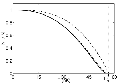
Figure 1: Condensate fraction versus temperature for $N=2\times 10^{6}$ atoms. The solid line corresponds to the method described in steps 1-4 in Section II. The Thomas-Fermi approximation is used to calculate the dashed line, as described in Ref. Williams2000 ; Minguzzi97a . The dot-dashed line is for an ideal Bose gas in the thermodynamic limit.

IV.2 Collective mode frequencies

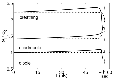
Figure 2: Condensate mode frequencies versus temperature for $N=2\times 10^{6}$ atoms. The dashed lines are the $T=0$ modes but for a changing number of condensate atoms $N_{c}(T)$. The solid line is the real part of the eigenenergies $\varepsilon_{i}$ obtained by solving (26).

We plot the collective excitation frequencies $\omega_{i}$ in Fig. 2 for the breathing $\{n=1,l=0,m=0\}$, dipole $\{0,1,m\}$, and quadrupole $\{0,2,m\}$ modes. The solid line corresponds to the numerical solution of the full coupled Bogoliubov equations in (26). For comparison, the dashed lines are obtained from the solution of (34) setting $2g\tilde{n}_{0}=0$ and using the value of $N_{c}(T)$ (as given by the dashed line in Fig. 1). In the Thomas-Fermi Stringari limit, the frequencies are given by the $T=0$ results, at all temperatures.

As $T$ approaches $T_{\rm{BEC}}$, $N_{c}(T)$ becomes very small and the solutions given by the dashed lines go over to the harmonic oscillator eigenstates—the breathing and quadrupole modes become degenerate at $\omega_{i}/\omega_{0}=2$. As $T$ decreases, the number of atoms in the condensate increases, so that the dashed line approaches the $T=0$ Stringari frequencies. The dipole mode frequency differs from the value $\omega_{i}=\omega_{0}$ expected for the Kohn mode since the thermal cloud is treated statically (see also Ref. Hutchinson97 ).

The deviation of the full solution (given by the solid lines) from the dashed lines is due entirely to the mean field of the static thermal cloud $2g\tilde{n}_{0}$. The upward shift in the frequencies (as illustrated in Fig. 2 for $N=2\times 10^{6}$) increases with $N$. Early studies Hutchinson97 ; Dodd98 ; Dodd98b of collective modes in the static Popov approximation considered much smaller systems, $N\sim 10^{3}$. In more recent work Bergeman2000 , the mode frequencies were computed for a much larger system of $N=2\times 10^{5}$ atoms. Although the thermodynamic quantities are very insensitive to the level of approximation used to treat the spectrum of the non-condensate atoms Giorgini97 ; Holzmann99 , the lowest-lying collective mode frequencies are clearly more sensitive. While we feel it is useful to show what our simple model gives for the frequency shifts, the shifts found in Refs.Hutchinson97 and Dodd98 , based on calculating $\tilde{n}_{0}({\bf r})$ more self-consistently, are much smaller than our model predicts. A good estimate clearly requires a more realistic theory Giorgini2000 ; Bergeman2000 , as discussed at the end of Section II.

IV.3 Damping due to inter-component collisions

In Fig. 3, we plot the damping rates $\gamma_{i}$ for $N=2\times 10^{6}$ atoms. In the main graph the damping of the breathing mode is shown, where the solid line comes from a full calculation based on (26) and the dashed line is calculated using the simplified expression in (49) derived in the Thomas-Fermi limit Williams2000 . As a reference point, we have indicated the temperature at which the condensate population $N_{c}(T)$ reaches $10^{4}$ atoms, where the ratio in (1) is $r_{\rm{HO}}/R_{\rm{TF}}=0.33$. The largest deviation, as expected, occurs close to $T_{\rm{BEC}}$ where the Thomas-Fermi approximation (1) used in deriving (49) starts to break down. The damping becomes very large as $N_{c}$ goes to zero close to the condensation temperature. This increase arises from the kinetic quantum pressure of the collective oscillation, i.e. the first term in (23).

In the inset of Fig. 3 we graph the damping rates for all three modes considered in Fig. 2. The similarity emphasizes the fact that the damping is fairly insensitive to the detailed form of the condensate normal modes, which suggests that the inter-component damping shown in Fig. 3 will not be significantly modified by a more accurate description of the static thermal cloud, in contrast to the frequency shifts.

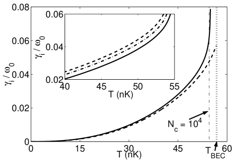
Figure 3: Damping rates versus temperature for $N=2\times 10^{6}$ atoms. In the main plot, the solid line corresponds to the full calculation of $\gamma_{i}=-{\rm{Im}}\varepsilon_{i}$ for the breathing mode as obtained by solving (26). The simplified TF expression (49) is given by the dashed line. In the inset, the full calculation of $\gamma_{i}$ is shown for the breathing (solid), dipole (dot-dashed), and quadrupole (dashed) modes.

Clearly as we approach $T_{\rm{BEC}}$, the condensate is becoming small while the thermal cloud is becoming more dominant. In this transition region, the nature of the excitations in a trapped Bose gas is quite complex. Since the condensate is disappearing, so are the collective modes and a theory based on (2) becomes inadequate.

V Discussion and Outlook

In summary, we have derived damped collective mode equations (25) for a condensate interacting with a static thermal cloud starting from the generalized GP equation derived in Ref. Zaremba99 . This mechanism is due to the lack of collisional detailed balance between the two components when the condensate is disturbed from equilibrium. In a previous article Williams2000 , we evaluated this damping in the large $N_{c}$ Thomas-Fermi limit and neglected the mean field of the non-condensate $2g\tilde{n}_{0}$. In Section IV we presented results of an explicit calculation of (25) and verified that the simplified TF expression (49) agrees quantitatively with the damping obtained from the full calculation, except very near $T_{\rm{BEC}}$ where $N_{c}(T)$ is becoming small.

Starting from the finite $T$ generalized GP equation (7), we formulated our calculation in terms of coupled Bogoliubov equations (25), in which the inter-component collision damping arises explicitly. We have used this opportunity to discuss some of the formal properties of these equations when damping is present. Such equations may be of interest in other problems when dealing with damping from the thermal cloud.

The effect of damping in the time-dependent Gross-Pitaevskii equation has been discussed in several different contexts Pitaevskii59 ; Hutchinson99 ; Choi98 . Many years ago, Pitaevskii Pitaevskii59 developed a phenomenological model for superfluid helium to describe the evolution of the superfluid toward equilibrium in the two-fluid hydrodynamic regime. This model has points of contact with the work in Ref. Zaremba99 . In Ref. Choi98 , a similar scheme was used to discuss damping of condensate modes in the collisionless region. In Ref. Hutchinson99 , damping terms were introduced into the GP equation to account for output coupling of condensate atoms from the trap as well as the exchange of atoms between the condensate and thermal cloud. Finally, in quite a different context, damped collective modes were calculated in Ref. Horak2000 for a condensate in an optical cavity.

Taking into account the dynamic mean field coupling between components, the collective modes of the system become a hybridization of condensate oscillations and non-condensate oscillations, so that one gets essentially a pair of in-phase and out-of-phase oscillations for each collective mode. For a given mode symmetry, the out-of-phase mode consists mostly of condensate oscillations with the collective motion of the non-condensate being less significant Zaremba99 . Our model calculations (and those of Ref. Williams2000 ) should be quite good for the intercomponent $C_{12}$ damping of such out-of-phase modes. In the other extreme, the in-phase Kohn mode Zaremba99 involves both the condensate and non-condensate moving together in local equilibrium, in which case $R({\bf r},t)=0$.

The dynamic coupling between the condensate and thermal cloud gives rise to damping of the condensate oscillations (known as Beliaev and Landau damping), which are quite distinct mechanisms from that considered in the present paper. Beliaev and Landau damping arise from dynamic mean-field effects, rather than collision terms such as $C_{12}$ or $C_{22}$ (for further discussion and references, see Refs. Giorgini2000 ; Williams2000 ). In a complete theory the condensate collective mode damping would be given by $\gamma_{\rm{tot}}=\gamma_{L}+\gamma_{B}+\gamma_{C}$, that is, Landau, Beliaev, and collisional (due to $C_{12}$) damping, respectively. Our model gives a good estimate of the $C_{12}$ damping $\gamma_{C}$. In our earlier work Williams2000 where we used the TFA, we compared the $C_{12}$ damping directly with Landau damping and found that $\gamma_{C}/\gamma_{L}\sim 0.3$ to $0.5$ for typical trap parameters.

We thank Sandy Fetter, Tetsuro Nikuni, Reinhold Walser, and Milena Imamović-Tomasović for useful discussions. This work was supported by NSERC.

Appendix A Collision integrals

The two collision terms on the right-hand side of (4) are given by Zaremba99

$$C_{22}[f] = {2g^{2}\over(2\pi)^{5}\hbar^{7}}\int\!\!d{\bf p}_{2}\int\!\!d{\bf p}_{3}\int\!\!d{\bf p}_{4}$$

$$\times \delta({\bf p}+{\bf p}_{2}-{\bf p}_{3}-{\bf p}_{4})\delta(\tilde{\varepsilon}_{p}+\tilde{\varepsilon}_{p_{2}}-\tilde{\varepsilon}_{p_{3}}-\tilde{\varepsilon}_{p_{4}})$$

$$\times \left[(1+f)(1+f_{2})f_{3}f_{4}-ff_{2}(1+f_{3})(1+f_{4})\right],$$

which is the usual Uehling-Uhlenbeck form of the Boltzmann collision integral describing collisions between thermal atoms, and

$$C_{12}[f,\Phi] = {2g^{2}n_{c}\over(2\pi)^{2}\hbar^{4}}\!\int\!\!d{\bf p}_{1}\!\int\!\!d{\bf p}_{2}\!\int\!\!d{\bf p}_{3}$$ (57)

$$\times \delta(m{\bf v}_{c}+{\bf p}_{1}-{\bf p}_{2}-{\bf p}_{3})\delta(\varepsilon_{c}+\tilde{\varepsilon}_{p_{1}}-\tilde{\varepsilon}_{p_{2}}-\tilde{\varepsilon}_{p_{3}})$$

$$\times [\delta({\bf p}-{\bf p}_{1})-\delta({\bf p}-{\bf p}_{2})-\delta({\bf p}-{\bf p}_{3})]$$

$$\times [(1+f_{1})f_{2}f_{3}-f_{1}(1+f_{2})(1+f_{3})],$$ (58)

describing the collisional exchange of particles between the condensate and non-condensate.

Appendix B Proof of Eq. 46

We give a formal proof that there is no first-order correction to the condensate frequencies from $\hat{\Gamma}$ in (25). From (43) and (44) we can write

$${\rm{Re}}\varepsilon_{1j}={1\over 2}{\int d{\bf r}w_{0j}^{\dagger}(\hat{M}^{\prime}+\hat{M}^{\prime\dagger})w_{0j}\over{\int d{\bf r}w_{0j}^{\dagger}\sigma_{3}w_{0j}}}.$$ (59)

From the explicit form of $\hat{M}^{\prime}$ given in (28), we obtain $(\hat{M}^{\prime}+\hat{M}^{\prime\dagger})=2i\sigma_{2}\hat{\Gamma}$, where

$$\begin{array}[]{ccc}\sigma_{2}&=&\left(\begin{array}[]{cc}0&-1\\ 1&0\end{array}\right).\end{array}$$ (60)

Then (59) becomes

$${\rm{Re}}\varepsilon_{1j}={i\int d{\bf r}w_{0j}^{\dagger}\sigma_{2}\hat{\Gamma}w_{0j}\over{\int d{\bf r}w_{0j}^{\dagger}\sigma_{3}w_{0j}}}.$$ (61)

We next define $w^{\prime}=\hat{\Gamma}w_{0j}$, which we expand in the basis of the undamped eigenmodes

$$w^{\prime}=\sum_{i}c_{i}w_{0i}.$$ (62)

Substituting this into (61) gives

$${\rm{Re}}\varepsilon_{1j}=i\sum_{i}c_{i}{\int d{\bf r}w_{0j}^{\dagger}\sigma_{2}w_{0i}\over{\int d{\bf r}w_{0j}^{\dagger}\sigma_{3}w_{0j}}}.$$ (63)

We make use of the general result Fetter72

$$\int d{\bf r}w_{0j}^{\dagger}({\bf r})\sigma_{2}w_{0i}({\bf r}) = \int d{\bf r}[v_{j}^{*}({\bf r})u_{i}({\bf r})-u_{j}^{*}({\bf r})v_{i}({\bf r})]$$ (64)

$$= 0,$$

which holds for all $i$ and $j$. Using this in (63) gives the final result (46).

References

- (1) E. Zaremba, T. Nikuni, and A. Griffin, Journ. Low Temp. Phys. 116, 277 (1999); see also T. Nikuni, E. Zaremba, and A. Griffin, Phys. Rev. Lett. 83, 10 (1999).
- (2) D. A. W. Hutchinson, E. Zaremba, and A. Griffin, Phys. Rev. Lett. 78, 1842 (1997).
- (3) R. J. Dodd, M. Edwards, C. W. Clark, and K. Burnett, Phys. Rev. A 57, R32 (1998).
- (4) R. J. Dodd, K. Burnett, M. Edwards, and C. W. Clark, Acta Physica Polonica A 93, 45 (1998).
- (5) J. E. Williams and A. Griffin, cond-mat/0003481 .
- (6) S. Stringari, Phys. Rev. Lett. 77, 2360 (1996).
- (7) F. Dalfovo, S. Giorgini, L. P. Pitaevskii, and S. Stringari, Rev. Mod. Phys. 71, 463 (1999).
- (8) H. T. C. Stoof, Journ. Low Temp. Phys. 114, 11 (1999).
- (9) R. Walser, J. Williams, J. Cooper, and M. Holland, Phys. Rev. A 59, 3878 (1999).
- (10) S. Giorgini, L. P. Pitaevskii, and S. Stringari, J. Low Temp. Phys. 109, 309 (1997).
- (11) J. E. Williams, Ph.D. thesis, University of Colorado at Boulder (1999), p. 149.
- (12) S. Giorgini, Phys. Rev. A 61, 063615 (2000).
- (13) T. Bergeman, D. L. Feder, N. L. Balazs, and B. I. Schneider, Phys. Rev. A 61, 063605 (2000), and references therein.
- (14) C. W. Gardiner and P. Zoller, Phys. Rev. A 61, 033601 (2000), and references therein.
- (15) L. P. Pitaevskii, Sov. Phys. JETP 35, 282 (1959).
- (16) D. A. W. Hutchinson, Phys. Rev. Lett. 82, 6 (1999).
- (17) S. Choi, S. A. Morgan, and K. Burnett, Phys. Rev. A 57, 4057 (1998).
- (18) A. L. Fetter, Ann. Phys. 70, 67 (1972).
- (19) J. P. Blaizot and G. Ripka, Quantum Theory of Finite Systems (The MIT Press, Cambridge, Mass., 1986).
- (20) A. Griffin, Phys. Rev. B 53, 9341 (1996).
- (21) A. L. Fetter and D. Rokhsar, Phys. Rev. A 57, 1191 (1998).
- (22) W. C. Wu and A. Griffin, Phys. Rev. A 54, 4204 (1996).
- (23) A. Minguzzi, S. Conti, and M. P. Tosi, J. Phys.: Cond. Matter 9, L33 (1997).
- (24) M. Holzmann, W. Krauth, and M. Naraschewski, Phys. Rev. A 59, 2956 (1999).
- (25) P. Horak and H. Ritsch, cond-mat/0002247 .
- (26) C. K. Law, H. Pu, N. P. Bigelow, and J. H. Eberly, Phys. Rev. Lett. 79, 3105 (1997).
- (27) J. J. Garcia-Ripoll and V. M. Perez-Garcia, Phys. Rev. Lett. 84, 4264 (2000).
- (28) D. L. Feder, M. S. Pindzola, L. A. Collins, B. I. Schneider, and C. W. Clark, cond-mat/0004449 .