Reversible Boolean Networks II: Phase Transitions, Oscillations, and Local Structures

Abstract

We continue our consideration of a class of models describing the reversible dynamics of $N$ Boolean variables, each with $K$ inputs. We investigate in detail the behavior of the Hamming distance as well as of the distribution of orbit lengths as $N$ and $K$ are varied. We present numerical evidence for a phase transition in the behavior of the Hamming distance at a critical value $K_{c}\approx 1.65$ and also an analytic theory that yields the exact bounds on $1.5\leq K_{c}\leq 2.$

We also discuss the large oscillations that we observe in the Hamming distance for $K<K_{c}$ as a function of time as well as in the distribution of cycle lengths as a function of cycle length for moderate $K$ both greater than and less than $K_{c}$. We propose that local structures, or subsets of spins whose dynamics are not fully coupled to the other spins in the system, play a crucial role in generating these oscillations. The simplest of these structures are linear chains, called linkages, and rings, called circuits. We discuss the properties of the linkages in some detail, and sketch the properties of circuits. We argue that the observed oscillation phenomena can be largely understood in terms of these local structures.

1 Introduction

Kauffman nets [1] have been used to model the complex behavior of dynamical systems ranging from gene regulatory systems [2, 3, 4], spin glasses [5, 6], evolution [7], social sciences [8, 9, 10, 11], to the stock market [12]. A Kauffman net consists of $N$ boolean variables or spins, each of which is either “+1” or “-1” at each time $t=0,1,2,\ldots$. We define $\sigma_{i}^{t}$ to be the value of the $i^{th}$ spin at time $t$. The system evolves through a sequence of states $\Sigma^{0},\Sigma^{1},\ldots,$ where

$$\Sigma^{t}=(\sigma^{t}_{1},\sigma^{t}_{2},\ldots,\sigma^{t}_{N})~{}.$$ (1)

There are $2^{N}$ different possible $\Sigma_{t}$’s.

The Kauffman net evolves according to

$$\sigma^{t}_{i}=F_{i}(\Sigma^{t-1})~{},$$ (2)

where $F_{i}$ is a boolean function with $K$ boolean arguments picked from among the $N$ possible arguments in ${\Sigma^{t-1}}$ and one boolean return. The $F_{i}$ for $i=1,2,\ldots,N$ are fixed during the evolution. The combination of them is called a realization. There are $(2^{(2^{K})})^{N}\binom{K}{N}^{N}$ different realizations for a net of $N$ elements with $K$ inputs [2].

After specifying a realization, one picks a starting state for the system; the network then evolves following equation (2).

Reference [13] (which we shall call paper I) introduces a time-reversible [14, 15, 16] boolean network model, [17] with dynamics governed by the equation

$$\sigma^{t+1}_{i}=F_{i}(\Sigma^{t})\sigma^{t-1}_{i}~{}.$$ (3)

Each time-reversible network realization has a corresponding dissipative realization with same functions and connections. In the reversible model substates $\Sigma^{t-1}$ and ${\Sigma^{t}}$ are both required to calculate $\Sigma^{t+1}$ [18], so the state of the system is $({\Sigma^{t-1}},{\Sigma^{t}})$, and the state space has $2^{2N}$ points.

Paper I studies how the distribution of cycle lengths generated by the time-reversible model scales with $N$ for different values of $K$. This paper investigates the cycle length distribution in more detail and also investigates the behavior of the Hamming distance [5, 19, 20] in this model. In the next section, we present both numerical evidence and analytic arguments that the behavior of the Hamming distance changes qualitatively and a phase transition occurs in the model at a critical value $K_{c}\simeq 1.65$. In section 3 we investigate how the realization average of the average number of cycles depends on the cycle length. For small $K$, cycle lengths divisible by integer powers of two and by three are much more likely than lengths that are products of larger prime numbers. Oscillations are also observed in the behavior of the Hamming distance as a function of time when $K$ is small. We explain these observations in terms of “local structures,” groups of spins whose dynamics do not depend on the state of any other spin in the system. In section  4, we discuss the two most important structures, linkages and circuits. We calculate Hamming distances and the cycle-length distribution for linkages. Our calculations for these structures are then connected back to the numerical observations, both for $K=1$ and for higher $K$.

2 Hamming distance in reversible Boolean nets.

In this paper we define the Hamming distance $D(t)$ to be the number of spins in two substates that are different at time $t$.

Consider two different time developments of a given realization of a system that are identical at $t=0$ and that have a single spin different at $t=1$. We obtain two series of configurations, called two paths of the system, and calculate $D(t)$, the Hamming distance between the two paths as a function of time $t$. In this subsection we consider the behavior of $\left\langle D(t)\right\rangle$, the Hamming distance averaged over different initial configurations and realizations, as a function of time $t$, for different values of the parameters $K$ and $N$ in our time-reversible model. We will find that when $K$ is small, at long times the maximum value of the Hamming distance saturates at a value that is independent of $N$ as $N\rightarrow\infty$, while when $K$ is sufficiently large, the saturation value is proportional to $N$ as $N\rightarrow\infty$. These two behaviors are separated by a phase transition at $K_{c}$, a critical value of $K$.

It is useful to define the normalized Hamming distance $\left\langle d(t)\right\rangle=\left\langle D(t)\right\rangle/N$, the average over realizations of the fraction of variables having different values in the two paths at time $t$. Below the phase transition, one finds that as $N\to\infty$ $\left\langle d(t)\right\rangle$ tends to zero for all $t$. while above $K_{c}$ the maximum of $\left\langle d(t)\right\rangle$ has a non-zero limit.

2.1 Hamming distance for $K=0$ and $K=N$

When $K=0$, if one starts with two copies of the system that are identical at time $t=0$ and have exactly one spin different at time $t=1$, the Hamming distance oscillates between $0$ and $1$ at all future times. When $K=N$, flipping a single spin changes an input of every spin, so that all spins have probability $1/2$ of being the same in the two paths at time $t=2$. Thus, when $K=N$, for all times $t\geq 2$, $\left\langle D(t)\right\rangle=N/2$, and $\left\langle d(t)\right\rangle=1/2$. Thus we see that the Hamming distance at long times $\left\langle D_{\infty}\right\rangle\equiv\lim_{t\rightarrow\infty}D(t)$, is independent of system size when $K=0$ and is proportional to the system size $N$ when $K$ is very large.

2.2 Hamming distance for intermediate $K$

To investigate intermediate $K$, we simulated reversible networks of 100, 1,000, 10,000 and 100,000 boolean variables for different $K$ values. For each case, 100 realizations were generated, and for each realization, one pair of paths with $D(0)=0$ and $D(1)=1$ was examined. Numerical results for $N=100,000$ are presented in figure 1. For all $K$’s, the Hamming distance first increases, then reaches a plateau, and finally oscillates about that plateau. For small $K$, large oscillations in $\left\langle D(t)\right\rangle$ are observed. In particular, when $K$ is small, $\left\langle D(t)\right\rangle$ is especially small when the time $t$ is a multiple of $2^{m}$ for integer $m$ (e.g., at $t=64$, $128$, and $256$). For larger values of $K$ these oscillations become much less pronounced.

Figure 1: Plot of $\left\langle D(t)\right\rangle$, the average over realizations of the Hamming distance as a function of time $t$, for systems with $N=100,000$ and different values of $K$. The starting initial conditions for each realization were chosen so that $D(0)=0$, $D(1)=1$. For visual clarity, this figure is split into two parts with different vertical scales. The left subfigure includes only $K$-values below or close to the critical value $K_{c}\simeq 1.65$, while the right subfigure includes $K$-values significantly above $K_{c}$.

This figure shows that $\left\langle D\right\rangle_{\max}$, the maximum value of the Hamming distance, exhibits a sharp jump as a function of $K$ at $K_{c}\approx 1.65$. This jump arises because, for $K>K_{c}$, $\left\langle D\right\rangle_{\max}$ is proportional to $N$ for large $N$, while for $K<K_{c}$, $\left\langle D\right\rangle_{\max}$ is independent of $N$ as $N\rightarrow\infty$. This behavior is shown in figure 2, which plots the maximum level of the normalized Hamming distance $\left\langle d\right\rangle_{\max}\equiv\left\langle D\right\rangle_{\max}/N$ as a function of $K$ for different $N$. Thus, $d_{\max}$ appears to act as an order parameter for a phase transition at $K_{c}\approx 1.65$.

Figure 2: Average of the peak of the normalized Hamming distance $\left\langle d\right\rangle_{\max}\equiv\left\langle D\right\rangle_{\max}/N$ as a function of $K$ for four decades of $N$ values. For each set of $N$ and $K$, we generated 100 pairs of paths with initial separations $D(0)=0$ and $D(1)=1$. Each of them is derived from a different realization and initial condition. For each pair of paths we calculate $D_{\max}$, the peak value of the Hamming distance, and then average this over realizations. The inset shows the behavior near criticality. We use these data to estimate that the critical value $K_{c}$ is about 1.65.

The phase transition that we observe at $K_{c}\simeq 1.65$ is of a percolative nature [21, 22, 23, 24]. When $K>K_{c}$, if one changes a few spins in the system, then information about the change spreads to more and more spins and eventually covers a nonzero fraction of all the spins in the system. When $K<K_{c}$, information remains localized within a few spins which tend to oscillate with periods which are powers of small prime integers. This phase transition is then connected with the percolation of information within the system.

The percolative nature of the phase transition in the reversible model has similarities to that observed in the dissipative Kauffman model [5, 25, 26], but there are differences. Specifically, consider two paths that are the time histories of a system realization that is started with two initial conditions that are almost the same, but having a small number of spin-values differing or ‘deviating’ from one another. The original Kauffman model is dissipative, so a spin whose values are deviating at early stages of the history may stop deviating as time goes on. However, a reversible system must undergo cyclic behavior. If a spin deviates at one time, it will do so at an infinite number of later times. In a reversible system, deviation is a permanent condition.

So we must ask how often a deviating spin triggers the deviation of others. Let $G$ be the average number of additional spins whose deviations are directly caused by a lone deviation in the system. The value of $G$ determines whether a few deviations will cause a chain reaction which will spread to the entire system. If $G>1$, the chain reaction will occur and the Hamming distance will eventually saturate at a value proportional to $N$. In the opposite case, $G<1$, a single deviation triggers less than one additional deviation on average, and the effect saturates long before the entire system is affected.

function	number of inputs	number	output for the input values
example	that affect output	in class	($+1$,$+1$)	($+1$,$-1$)	($-1$,$+1$)	($-1$,$-1$)
+1	$0$	$2$	$+1$	$+1$	$+1$	$+1$
$\sigma_{1}$	$1$	4	$+1$	$+1$	$-1$	$-1$
$\sigma_{1}\sigma_{2}$	2	2	$+1$	$-1$	$-1$	$+1$
$\sigma_{1}~{}~{}\text{or}~{}~{}\sigma_{2}$	$q$	8	$+1$	$+1$	$+1$	$-1$

Table 1: The different classes of functions, $F(\sigma_{1},\sigma_{2})$, for $K=2$. The classes are defined by the symmetry operations of spin flip and interchange of the two spins.

2.3 Bounds on the critical value $K_{c}$.

Though we have not calculated exactly the branching ratio $G$ for this chain reaction, we can prove that $1.5<K_{c}<2$. We first prove that $1<K_{c}\leq 2$, and then refine the argument to show that $1.5<K_{c}<2$.

We define systems with fractional $K$ to be composed of elements that have probability $[K]+1-K$ of having $[K]$ inputs and probability $K-[K]$ of having $[K]+1$ inputs, where $[x]$ is the largest integer less than or equal to $x$. (This then defines $K$ as the average number of inputs, since $([K]+1-K)+(K-[K])=1$ and $[K]([K]+1-K)+([K]+1)(K-[K])=K$). The growth rate $G_{K}$ is the average

$$G_{K}=([K]+1-K)G_{[K]}+(K-[K])G_{[K]+1}~{}.$$ (4)

Thus we need only calculate $G_{K}$ for integer $K$.

2.3.1 $K_{c}>1$.

We can see immediately that deviations will not percolate if $K$ is less than or equal to one. When $K=0$, every spin is independent of its inputs, so $G_{K=0}$=0. When $K=1$, there are four different possibilities for $F_{i}(\sigma)$, namely $1$, $-1$, $\sigma$, and $-\sigma$. In our model all functions occur with equal probability, so a deviation in the spin $\sigma$ triggers a deviation in the spin $\sigma_{i}$ to which it is an input with probability $1/2$. Thus the growth factor for $K=1$ is

$$G_{K=1}=0.5~{}.$$ (5)

The growth factor for $K$ between $0$ and $1$ is just $KG_{K=1}$, so for $K$ less than or equal to one the system must be below its percolation threshold.

2.3.2 $K_{c}<2$.

For any $K$, changing any one of the $K$ arguments of a function $F_{i}({\Sigma})$ has a $50\%$ chance of flipping its output value. Therefore, a deviation of a single spin will, at the very next step, cause an average of $K/2$ deviations. Later steps may cause further deviations, but considering only this initial step certainly bounds the growth factor:

$$G_{K}\geq K/2~{}.$$ (6)

Thus, when $K>2$ the growth factor $G_{K>2}>1$, so that the deviation will spread to a nonzero fraction of the entire system.

At first sight, it appears that $K=2$ is the marginal, or critical case. That is wrong. Information will also percolate through the entire system when $K=2$. In the previous paragraph, we considered the further deviations induced in the very next step after the deviation of a given spin. These effects were enough to ensure that at least $K=2$ is marginal. However, a deviation can have a delayed further effect, producing additional deviations beyond the one we have already calculated. These additional deviations then permit information to percolate through the entire system for $K=2$.

To see this result, we need only establish one case with a further, delayed, deviation. Notice Table 1. Consider a situation in which spin number $3$ is determined by the “or” function shown on the last line in the table. Assume that input spin $1$ has just deviated and input spin $2$ has the value $+1$ on both paths. Now spin $3$ does not deviate at this step. However, if at a later stage spin $2$ takes on the value $-1$, that will induce a delayed deviation of spin $3$. Since situations like these occur with non-zero probability, and increase the value of $G_{K=2}$ beyond the value shown in equation 6, the case $K=2$ is above the percolation threshold.

2.3.3 $K_{c}>1.5$.

Since we know $1<K_{c}\leq 2$, we need only consider values of $K$ between $1$ and $2$. We have already calculated $G_{K=1}$ and a lower bound to $G_{K=2}$; now we wish to consider $G_{K=2}$ in more detail.

Let us estimate the average number of additional deviations produced by one deviated spin. The growth rate $G_{K=2}$ is $2N$ times the probability that a spin $\sigma$ is induced to deviate when one of its two inputs has deviated, which is in turn the sum of products of the likelihood of a function choice times the probability that the function gives different outputs with one deviated input. Of the sixteen two-input functions $F(\sigma_{1},\sigma_{2})$, two functions ($\pm 1$) depend on zero inputs, four functions ($\pm\sigma_{1}$, $\pm\sigma_{2}$) depend on one input (they change output if one input is changed but not the other one), and two functions ($\pm\sigma_{1}\sigma_{2}$) depend on two inputs (they change if either input is changed). The remaining eight functions are like the “or” function; they depend upon one argument only for a particular value of the other argument. (See Table 1.) Therefore,

$$G_{K=2}=\frac{2\times 0+4\times 1+2\times 2+8\times q}{16}~{},$$

where $q$ is the unknown effective number of inputs of the functions like “or”. We overestimate $q$ by saying that these functions all behave exactly as if they had two inputs. This estimate then gives us

$$G_{K=2}\leq\frac{3}{2}~{}.$$ (7)

Putting together our results from equations 5, 4 and 7, we find that

$$G\leq(2-K)0.5+(K-1)1.5=-0.5+K~{}.$$ (8)

This overestimate gives us a marginal growth rate at $K=1.5$, which yields a lower bound to the critical value $K_{c}\geq 1.5$. Our best numerical evidence is computed from the data shown in figure 2 and gives $K_{c}=1.65\pm 0.10$. This result is, of course, in agreement with the exact bounds.

3 Oscillations in orbit period distributions

In this section we present our numerical results for cycle length distributions, and give a qualitative explanation of what we are seeing. When $K$ is small but larger than $K_{c}$, the number of cycles does not depend smoothly on length. Instead, cycles whose lengths are divisible by small integer powers of two and by three predominate. As $K$ is increased, the cycle length distribution becomes smoother. We relate this trend to the evolution in the connectivity of the network as $K$ is increased. When $K$ is small, we can have small clusters of spins that are only weakly coupled to the other spins in the system. These local structures are shown to have a characteristic effect of yielding cycle lengths divisible by small factors such as two and three. As $K$ increases, all the spins tend to be in a single large cluster with complex interactions, and local structures become much less likely. This leads to a much smoother cycle length distribution.

3.1 Simulation results for cycle length distributions

Figure 3 shows the distribution of cycle lengths for intermediate $K$ values and $N=10$.

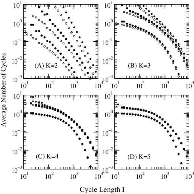
Figure 3: Log-log plots of numbers of cycles per realization, averaged over realizations, as a function of cycle length $l$ for $N=10$ and for $K=2$, $3$, $4$, and $5$. For each $K$, all cycles are enumerated from each of 25600 realizations. Note the different branches arising from oscillations in these functions. The different point styles distinguish the different divisors of the $l$-values. They are: $l=0\mbox{ mod }4$ (circles), $l=2\mbox{ mod }4$ (squares) and $l=1\mbox{ mod }2$ (diamonds). Filled symbols have $l=0\mbox{ mod }3$, while open symbols denote $l$ not divisible by three.

The distribution oscillates strongly when $K$ is small. As $K$ is increased, the oscillations diminish and the distribution eventually converges to the random hopping behavior discussed in Paper I [13]. A complex oscillation pattern in the distribution is evident, particularly for the cases $K=2$ and $K=3$. Several different branches are observed, which reflect periods which are or are not divisible by small powers of two and of three. The oscillations at moderate $K$ in the reversible model are significantly more pronounced than those observed in dissipative Kauffman models [27]. The amplitude of the oscillation diminishes as $K$ increases, and as $K$ approaches $N$, the distribution approaches the two-branch structure (due to an even-odd oscillation) calculated in the $K=N$ case in Paper I.

To see the oscillatory structure in more detail, we show in Fig. 4 an enlarged plot which shows the number of cycles for the region extending from $l=360$ to $l=408$. The most likely cycles fall into three main branches, which in decreasing order of probability satisfy $l=0\mbox{ mod }4$, $l=2\mbox{ mod }4$, and $l=1\mbox{ mod }2$. Each main branch is further split, with cycle-lengths that are multiples of three being more likely. Thus, the cycle lengths that are divisible by $24$ occur with the highest likelihood.

This oscillation is not a small effect. Figure 4 demonstrates that cycle lengths divisible by $24$ are more than two orders of magnitude more common than any odd cycle length in this range of $l$. Thus we see a marked tendency for orbit periods to contain factors of $2^{n}$ for small integer $n$ and of $3$.

Figure 4: Enlarged plot on a semilog scale of the realization average of the number of cycles of length $l$ versus $l$ for $N=10$ and for $K=2$. The oscillation structure is highlighted by showing only the region extending from $l=360$ to $l=408$. The main structure of the figure consists of three branches, which in decreasing order of probability satisfy: $l=0\mbox{ mod }4$ (circles), $l=2\mbox{ mod }4$ (squares) and $l=1\mbox{ mod }2$ (diamonds). Filled symbols are used for lengths evenly divisible by three and open symbols for those that are not. The plotting symbols are the same as in Fig. 3.

3.2 Characterizing the oscillations in the cycle length distribution

We now look for a quantitative measure of the amount of oscillation in cycle length, so that we can see how it changes as a function of $K$. More specifically, we wish to ask whether we can understand how the oscillations go away for large $K$.

For small $K$, the even cycles predominate. It is very likely indeed, that among the many independent localized stuctures in oscillation at least one will give a period two oscillation, which will then be observed in the overall period of the system. To show this, we plot in Figure 5 the ratio of the number of even cycles to the number of odd ones for two different system sizes, $N=10$ and $N=7$.

Figure 5: The ratio of the number of even cycles to that of odd ones plotted against $K$ for $N=7$ and $N=10$. For each $K$ and system size, all cycles are enumerated in each of $25,600$ realizations. For small $K$ values, the ratio increases rapidly as the system gets larger, while for large $K$, the ratio stays at a level above unity, which depends much more weakly on system size.

For large $K$, the global behavior forces the number of even cycles to be greater than the number of odd ones, but the effect depends very weakly on $N$. For smaller values of $K$ the ratio becomes much larger, and has substantial $N$-dependence.

To parametrize the oscillation structures for different $K$ values, we first separate the domain of possible cycle lengths into segments of length $P$. Based on the argument about the appearance of factors of small powers of $2$ and $3$ in the system’s periods, and also the observation in Fig 4, we choose $P$ to be 24. We also require the $i$th segment to start at $24i$ and thus the 24 elements of the segment are $24i+r,\quad r=0,1,\ldots,23$. Paper I discusses how correlated fluctuations in the number of mirrors could produce an even-odd oscillation in the number of cycles. In this paper, the even-odd oscillations (exhibited in figure 4 of Paper I) are just a distraction. To eliminate the even-odd effect due to the correlated fluctuations in the number of mirrors, we define $q_{i}(r)$ to be the proportion of cycles of period $24i+r$ among all the even cycles in the segment when $r$ is even, and among all the odd ones when $r$ is odd. We then average $q_{i}(r)$ over segments of which the number of both even cycles and odd cycles are observed more than 100 times in our simulation (complete enumeration of 25,600 realizations), and thereby obtain the functions $Q(r)$.

The functions $Q(r)$ are plotted separately for even and odd values of $r$ in figure 6. For $K=2$ we can see very strong oscillations as a function of $r$ in both plots. As expected, factors of three and of four are favored (this plotting method does not show the oscillations with period two). As $K$ is increased, the $r$-dependence becomes much weaker.

Figure 6: $Q(r)$ as a function of $r$. Top: even cycles. Bottom: odd cycles. High $Q$ values mean high likelihood of observing a cycle length with certain residues. Numerical data were obtained by complete enumeration of 25,600 realizations for each $K$.

To characterize the strength of the oscillation for a given $K$ using a single parameter, we order $r=0,1,2,\cdots,P-1$ in the increasing order with respect to $Q(r)$ and index them as $r_{1},r_{2},...,r_{P}$. The Gini coefficient [28], a measure of the inequality between the $P$ values of $Q(r)$, is defined as

$$G=1-\frac{2\sum^{P-1}_{i=1}\sum^{i}_{j=1}Q(r_{j})}{(P-1)\sum^{P}_{j=1}Q(r_{j})}.$$ (9)

When all the $Q(r)$ are equal, $G$ takes on its minimum value, $G=0$; when only $Q(r_{P})$ is nonzero, so that the distribution of $Q(r)$ is extremely inequitable, then $G=1$.

The Gini coefficients as a function of $K$ with $N=10$ and $P=24$ are shown in figure 7. Notice that there are separate curves for even and odd values of $r$. We see that the Gini coefficient is large for small $K$ and decreases rapidly as $K$ gets larger, showing values indistinguishable from zero for $K$ above $5$.

Figure 7: Our Gini coefficients measure the size of oscillations in the number of cycles as a function of length. They are obtained by complete enumeration of 25,600 realizations for each $K$ and plotted here, with even and odd cycles separated. When $K=1$, the only odd cycles observed are of length $3$ and thus $G=1$ for the odd cycles.

3.3 Local structures

In this section, we discuss why cycle lengths are so likely to be evenly divisible by small powers of two and by three. When $K>K_{c}$, the influence of a single spin flip percolates and reaches a finite fraction of the entire spins in the lattice. We can then imagine that a nonzero fraction of all the spins in the system fall into a main connected cluster, one with many complex linkages among the different spins in the cluster. We depict this in Figure 8, in which the ‘C’ denotes the connected cluster. It is further indicated by the surrounding curve.

3.3.1 Isolated structures

But $K$ is not infinite. There will be spins in the system which are only weakly coupled in to the rest. For example, there will be spins which are simply uncoupled to any others. One such spin is indicated by the ‘$I_{0}$’ in the figure. This spin has a function $F_{i}(\Sigma)$ which is simply $\pm 1$, independent of all the spins. Thus, this coupling has an effective $K$-value of zero. It is possible that this isolated spin does not affect any other spins in the system. It can also happen that the isolated spin can affect one or several spins in the cluster. We show this with the situation labeled as ‘$I_{1}$’. The effect of the two situations is rather similar.

There are other examples of weakly coupled spins. But the effect of the isolated spin can be calculated in full detail, and will serve to illustrate the qualitative nature of localized-structure-effects.

First of all notice that for large $N$ there will be many such isolated spins. For a given value of $K$ the probability that a spin is assigned the function $-1$ or $+1$ is $2^{(1-2^{K})}$, so that the average number of such spins will be

$$p=2^{(1-2^{K})}N~{}.$$

This number must be large for sufficiently large $N$. A spin with input function $-1$ is in a period-4 cycle, while a spin with input function $+1$ is in a cycle of period 1 for half its possible initial conditions and in a cycle of period 2 for the other half. Thus, for large $N$ there will on average be many isolated spins in cycles of length two or four. It follows that it will be overwhelmingly likely that the cycle length of the entire system will be divisible by two.

Our $N$’s are not very large. But $N=10$ is large enough so that isolated spins are likely, and they play a substantial role in making our cycle-lengths mostly divisible by several factors of two. As figure 5 demonstrates, when $K$ is small, the ratio of even to odd cycles increases rapidly as $N$ is increased, consistent with the idea that local structures have a substantial effect at small $K$.

Factors of three are only slightly harder to obtain. Imagine, for example, a spin coupled only to itself via

$$F_{i}({\Sigma})=\pm\sigma_{i}~{}.$$

One initial condition for such a spin results in a cycle length of one, while the other three result in a cycle length of three. These and other structures can then give us our observed factors of three.

Other isolated structures can be formed that have a substantial influence on system properties. For example, one can have a structure like the linkage ‘$L_{0}$’ shown in Fig. 8. A linkage is a sequence of spins linked together by coupling of the form $\pm\sigma$. The arrow indicates that the value of the spin on at the tail changes the values of the spin at the head. A linkage like ‘$L_{0}$’ has no effect on the cluster. One can also have a linkage like ‘$L_{1}$’ which directly influences the cluster. We shall discuss the effect of linkages in more detail in the next chapter. For now we merely point out that these, and other, more complex structures have a simple effect upon the overall periods of the system. Each small isolated structure has its own short period. The motion for the entire system must be a multiple of the periods for each of the isolated structures. Since the small structures all tend to have periods two and three and four, it is no wonder that these factors appear very often in the observed periods of Fig. 3.

Figure 8: This figure shows the simplest kinds of clusters. The arrows show the flow of information. The cluster inside the circle labeled ‘C’ is connected. That means it contains many spins intimately linked by complex interactions. The clusters labeled ‘$I_{0}$’, ‘$I_{1}$’ and ‘$I_{2}$’ are single spins, isolated from the influence of any others. As we have depicted them, the ‘$I_{0}$’ conveys no information to the connected cluster while ‘$I_{1}$’ brings information from the isolated cluster to the connected cluster. We also depict the linkages ‘$L_{0}$’ and ‘$L_{1}$’, slightly more complex structures which also undergo their own independent motion. The $D$’s indicate dangling structures.

3.3.2 Dangling structures

It is also possible to have isolated structures which are influenced by the connected cluster but do not influence it themselves. For example, consider a spin, $\sigma_{i}$, whose input function $F_{i}({\Sigma})$ depends only on spins that are not causally related to $\sigma_{i}$. Then the extra spin ‘dangling on’ the cluster produces a simple effect upon the periods of the entire system. To deal with this situation, we prove a theorem.

Theorem 1.

Consider two sequences $F^{t}$ and $\sigma^{t}$. We assume that both of them are sequences of $+1$’s and $-1$’s, that $F^{t}$ is periodic with period $T_{F}$, and that the $\sigma$’s depend upon the $F$’s according to

$$\sigma^{t+1}=F^{t}\cdot\sigma^{t-1}.$$ (10)

Then $\sigma$ is periodic with period $T_{\sigma}$, where $T_{\sigma}$ can only be $T_{F}$, $2T_{F}$, or $4T_{F}$.

We prove this by showing that (A) $T_{\sigma}$ divides $4T_{F}$ evenly, and (B) $T_{F}$ divides $T_{\sigma}$ evenly. To prove (A), note that

$$\sigma^{t+2T_{F}}=\Pi(t)~{}\sigma^{t}~{},$$ (11)

where

$$\Pi(t)=F^{t+2T_{F}-1}F^{t+2T_{F}-3}\ldots F^{t+3}F^{t+1}~{}.$$ (12)

When $T_{F}$ is odd, $\Pi(t)$ is a product over a full period of the $F$’s. Therefore, it is independent of time. If it is +1, the sequence of $\sigma$’s repeats after $2T_{F}$. If it is -1, then $\sigma^{t}$ repeats after $4T_{F}$. If $T_{F}$ is even, then

$$\Pi(t)=\left[\Pi_{m=1}^{T_{F}/2}F^{t+T_{F}-2m+1}\right]^{2}=1~{}.$$

Therefore, when $T_{F}$ is even, $\sigma^{t+2T_{F}}=\sigma^{t}$. Thus, for both even and odd $T_{F}$, $\sigma$ is periodic with a period $T_{\sigma}$ that divides $4T_{F}$ evenly.

Now we prove (B), that $T_{F}$ divides $T_{\sigma}$ evenly. For any $t$, we have

$$\sigma^{T_{\sigma}+t} = \Pi^{\prime}(t)~{}\sigma^{t}\text{\quad with}$$

$$\Pi^{\prime}(t) = F^{T_{\sigma}+t-1}\cdots F^{t+3}F^{t+1}~{}.$$

The periodicity of $\sigma$ implies that $\Pi^{\prime}(t)=1$ for all $t$. Note that, for all $t$,

$$\Pi^{\prime}(t+2)=F^{T_{\sigma}+t+1}~{}F^{t+1}~{}\Pi^{\prime}(t)~{}.$$

Thus, $F^{T_{\sigma}+t}=F^{t}$ for all $t$, and $T_{F}$ must divide $T_{\sigma}$ evenly.

Q.E.D.

Theorem 1 enables us to see additional mechanisms for the multiplication of cycle lengths by factors of two and four. Look at the structures dangling from the end of a connected cluster as also shown in Fig. 8. A dangling cluster consisting of a single spin can multiply the periods produced by the connected cluster by a factor of one, two, or four. The two-spin dangle can, at most, produce a lengthening by a factor of eight. Thus, these dangles produce additional mechanisms for the appearance of factors of two in the period of the entire system.

4 Some local structures

In the preceding two sections we saw that small $K$ reversible Boolean nets exhibit large oscillations, both in the behavior of the Hamming distance as a function of time and the orbit period distribution as a function of period $l$. We explained the latter as an effect of small localized structures. In this section, we discuss the localized structures in more detail. Our purpose is both to explain the oscillations exhibited above, as well as to explore some of the structures’ statistical properties.

4.1 The structures and their coupling

Two kinds of elements, depicted in figure 9, serve as a basis for a description of the behavior at $K=1$. These same elements, called linkages and circuits, may also be expected to dominate the behavior at small $K$. Others have discussed the effect of structures like these for the dissipative Kauffman model[26, 29, 30, 31]. The behavior is, of course, different in the reversible case.

4.1.1 The structures

A linkage is $L$ spins, $\sigma_{j},~{}j=1,\ldots,L$, coupled together in a linear array. The first spin has an input function, $F_{1}$, that is either $+1$ or $-1$. Information is transferred from one spin to the next, for all $j$ bigger than one, with a coupling function

$$F_{j}(\Sigma)=\pm\sigma_{j-1}\qquad\mbox{for }\qquad j=2,3,\ldots,L~{}.$$ (13)

A circuit of length $L$ is like a linkage except that the last spin is coupled to the first with

$$F_{1}(\Sigma)=\pm\sigma_{L}.$$ (14)

These basic structures may also be tied together, as for example, in the tree and the tadpole shown in figure 10. In this section, we shall analyze the basic structures. We shall, however, not explore the effects of the multiplicity of structures which can be present at one time, nor of the different ways these structures can be coupled.

Figure 9: Two kinds of basic structures. Each circle represents a spin; the spin at the end of an arrow depends on the spin from which the arrow starts.

Figure 10: Possible ways in which the basic structures may be tied together. Both the tree and the tadpole are possible structures at K=1. However, if the arrows were reversed, these structures would only become possible at higher $K$.

4.1.2 Local structures at $K=1$.

For $K=1$, since two of the four Boolean functions of one variable do not depend on the input, half of all spins have dynamics that do not depend on the state of any other spin. Therefore, typical local structures in networks with $K=1$ tend to contain only a few spins.

For a given $K$, the numbers of linkages and circuits depend only on the placement of the couplings and on the function choices, and do not depend on whether the dynamical equation is dissipative or reversible. Flyvbjerg and Kjaer [30] have calculated the number of circuits of length $L$ exactly in the context of the dissipative Kauffman model. However, they did not calculate the number of linkages, doubtless because linkages of all lengths have trivial dynamics in the dissipative Kauffman model.

The number of spins in linkages is of order $N$, while the number of spins in circuits is of order unity. This scaling follows readily via the following argument. When $K=1$ each spin has one input chosen from $N$ possibilities, and the spin depends on the input only if its function is $\pm\sigma$, which occurs with probability $1/2$. The probability that a spin depends on any other spin is of order one, while the probability that it depends upon itself is of order $1/N$. Consequently, there are of order $N$ spins linked to other spins, but only of order one spin linked to itself. An extension of this argument implies that there are of order $N$ linkages, but only of order one circuit in the entire system. Tree-like structures can be formed from linkages alone, and tadpoles from combinations of linkages and circuits. The former have a behavior which is qualitatively similar to a single linkage, the latter have properties which are closer to that of circuits.

4.2 Theorems for the analysis of linkages and circuits.

There are three theorems which greatly facilitate our work with linkages and circuits.

We have already stated one of these as our theorem 1 in Sec. 3. This theorem tells us how the period of a base structure is affected by a spin dangling on the end. The period of the base is multiplied by one or two if the base period is even and one, two, or four if it is odd. By direct calculation, one sees that a linkage of length one will have a period of one or two or four. Hence, all linkages have periods that are integer powers of two.

The other two theorems apply more specifically to linkages and circuits. They are:

Theorem 2 (Equivalent Structure Theorem).

For a linkage or a circuit, switching the function assignment $F_{j}(\sigma)$ from $\sigma$ to $-\sigma$ does not affect the dynamics of the structure in the sense that we can always find a one-to-one map from the state-space of the local structure to itself, relating a cycle before switching the function assignment to a cycle with the same cycle length after the switch.

Proof: For each $F_{j}(\sigma)$ which has the value $-\sigma$, change the variable $\sigma_{j-1}$ into $-\sigma_{j-1}$. Q.E.D.

Note: This change leaves all Hamming distances and cycle lengths unchanged. Hence, for the examination of these quantities we need only consider the case in which the linkage functions are $F_{j}(\Sigma)=\sigma_{j-1}$ and not the cases in which $F_{j}(\Sigma)=-\sigma_{j-1}$.

Theorem 3 is a superposition principle that applies to systems with $K=1$.

Theorem 3 (Superposition Principle).

Consider a network with $K=1$. The equations of motion are of the form

$$\sigma_{j}^{t+1}=F_{j}(\Sigma^{t})\sigma_{j}^{t-1}~{},$$ (15)

Let

$$f_{j} = 1\text{~{}~{}if~{}~{}}F_{j}(\Sigma^{t})=+1\text{~{}or~{}}\sigma_{i}^{t}\text{\quad for some~{}}i(j)~{}$$

$$f_{j} = -1\text{~{}~{}if~{}~{}}F_{j}(\Sigma^{t})=-1\text{~{}or~{}}-\sigma_{i}^{t}\text{\quad for some~{}}i(j)~{}.$$ (16)

Let $\sigma_{j}^{t}$ and $\mu_{j}^{t}$ both be solutions to the equations of motion for the same realization of the $K=1$ couplings. Then

$$\rho_{j}^{t}=f_{j}~{}\sigma_{j}^{t}\mu_{j}^{t}$$ (17)

is also a solution.

Proof: This multiplication rule can be immediately verified on each bond in equation 15. Therefore it must be true globally.

Note that the change of variables from $\sigma$ to $(\ln f~{}\sigma)/(i\pi)$ converts this multiplicative superposition into the kind of additive superposition principle which arises for all linear equations.

4.3 Hamming distance for linkages and circuits.

One can make considerable progress in the Hamming distance problem for long linkages and circuits. The Equivalent Structure Theorem implies that for each $L$ we need to study only one circuit problem and two linkage problems. The latter differ by their first coupling, which can take on the two values $F_{1}=\pm 1$.

First we show that the Hamming distance can be obtained by solving a single linkage or a circuit problem. Consider a linkage or circuit with a solution $\Sigma^{t}=\{\sigma_{j}^{t}\}$, and let $\mathcal{M}^{t}=\{\mu_{j}^{t}\}$ be another solution with initial conditions that are identical to those for $\Sigma^{t}$ at $t=0$ and have, at $t=1$, a single spin different, the spin with index $J$. Then defining

$$\rho_{j}^{t}=\sigma_{j}^{t}\mu_{j}^{t}~{},$$ (18)

all the values of $\rho_{j}^{0}$ and $\rho_{j}^{1}$ are unity except for $\rho_{J}^{1}=-1$. The variable $\rho_{j}^{t}$ is minus one whenever the two paths differ, so the Hamming distance between $\mathcal{M}$ and $\Sigma$ at time $t$ is

$$D(t)=\sum_{j=1}^{L}\frac{1}{2}(1-\rho_{j}^{t})~{}.$$ (19)

The subsequent history of $\rho$ is calculated starting from the initial data and the equations of motion

$$\rho_{j}^{t+1}=\rho_{j-1}^{t}\rho_{j}^{t-1}\text{\quad for \quad}i=2,3,\dots,L~{}.$$ (20)

For the linkage, all the $\rho_{j}^{t}$ are one if $j<J$ and $(-1)^{t}$ if $j=J$. The picture just stops short at $i=L$; nothing is meaningful to the right of this value of $i$. For the circuit, we apply the periodic boundary conditions $\rho_{j+L}^{t}=\rho_{j}^{t}$.

Figure 11: Cascading Effect of a Single Spin Flip. Here, $\rho_{j}^{t}$ is plotted for a situation in which the flip occurs in a very large linkage or circuit. The grey squares denote $\rho=1$; the black, $\rho=-1$.

The result for a very large linkage or circuit is shown in Figure 11. This figure shows the familiar Sierpinski gasket [32, 33], rotated ninety degrees from the conventional representation. In fact, equation 20 is equivalent to rule $90$ in Wolfram’s cellular automaton scheme, which is known to generate a Sierpinski gasket [34].

Figure 12 shows a plot of Hamming distance $D(t)$ versus iteration number $t$ for the gasket. The distance is unity at times $2^{n}$ and its average in the binary decade $[2^{n},2^{n+1}]$ is $\left(\frac{3}{2}\right)^{n-1}$. Thus, this average increases as $t^{(\log_{2}3-1)}\approx t^{0.59}$ [35]. The maximum value of $D(t)$ in the range $[2^{n-1},2^{n}]$ is the Fibonacci number $F_{n}$, where $F_{1}=1$, $F_{2}=2$, and $F_{j}=F_{j-1}+F_{j-2}$, which scales as $t^{\log_{2}\left(\frac{1+\sqrt{5}}{2}\right)}\approx t^{0.69}$. Both the average of $D(t)$ and the maximum value of $D(t)$ in each binary decade can be obtained analytically by exploiting the fractality and symmetry properties of the Sierpinski gasket.

To calculate the Hamming distance in a linkage of finite length $L$, started by flipping a spin $J$ sites into the linkage, note that no information travels to sites $\sigma_{i}$ with $i<J$, and that the dynamics are cut off at the last site $i=L$. If the distance from $J$ to the right hand boundary is between $2^{n}$ and $2^{n+1}$, the motion repeats with a period $2^{n+2}$. We shall see below how this information may be converted into statements about the distribution of periods for the linkage.

The Hamming distance behavior for the circuits can be understood by seeing the circuit picture as one in which the gasket picture is folded onto itself an infinite number of times, with the folding distance being, $L$, the size of the circuit. Because two superposed black dots cancel and make a gray one, the folding can produce complex patterns. Nonetheless, we know that the Hamming distance is unity at times which are of the form $2^{n}$, for integer $n$, since at these times there is but one black dot. Furthermore, the typical or average Hamming distance must grow no more rapidly than $t^{0.59}$, since this growth is bounded above by the number of black dots in the non-overlapping gasket. We shall come back to this fold-over picture in order to assess periods of circuit motion.

Figure 12: Numerically calculated Hamming distance versus time for a linkage with Sierpinski gasket dynamics (solid line). The average of the Hamming distance in each binary decade grows as $t^{\left(\ln_{2}3\right)}\approx t^{0.59}$ (dotted line), while the maximum value of the Hamming distance in each binary decade grows as $t^{\log_{2}\frac{1+\sqrt{5}}{2}}\approx t^{0.69}$ (dashed line).

		number of cycles with period
L	$F_{1}$	$l=$1	$l=$2	$l=$4	$l=$8	$l=$16
1	1	2	1
2	1	2	1	3
3	1	2	1	3	6
4	1	2	1	3	30
5	1	2	1	3	30	48
6	1	2	1	3	30	240
7	1	2	1	3	30	1008
8	1	2	1	3	30	4080

Table 2: Numbers of orbits of different periods for linkages of lengths $L$ from $1$ to $8$ with $F_{1}=+1$.

$L$	Cycle Length $l$’s (Multiplicities)
1	1(1) 3(1)
2	1(1) 3(1) 6(2)
3	1(1) 3(1) 5(3) 15(3)
4	1(1) 3(1) 6(2) 12(20)
5	1(1) 3(1) 17(15) 51(15)
6	1(1) 3(1) 5(3) 6(2) 10(24) 15(3) 30(126)
7	1(1) 3(1) 7(9) 9(28) 21(9) 63(252)
8	1(1) 3(1) 6(2) 12(20) 24(2720)

Table 3: Complete enumeration of all possible orbits for circuits of lengths $L\leq 8$. The numbers in the body of the table are the possible cycle lengths and, in parentheses, the number of different cycles of that length.

4.4 Cycle length distributions for linkages.

Table 2 shows the distribution of cycle-lengths for the first few linkages. As expected, the linkages all have periods which are powers of two. We now calculate the distribution of cycle-lengths.

Figure 13: Primitive sequences ${{}^{(+-)}\mathcal{S}_{L}^{t}}$, ${{}^{(-+)}\mathcal{S}_{L}^{t}}$, and ${{}^{(++)}\mathcal{S}_{L}^{t}}$ for a linkage of length $L=20$.

First we show that the orbit period of a linkage is determined entirely by the root spin, defined to be the spin $\sigma_{J}$ with the smallest value of $J$ that has an initial condition other than $(+1,+1)$. It is useful to define the $(-+)$ primitive sequence ${{}^{(-+)}\mathcal{S}_{L}^{t}}$ for a linkage of length $L$ to be the values $\{\sigma_{i}^{t}\}$ for $i=1,....L$, $t=2,3,....$ that one gets starting a linkage of length $L$ with $F_{1}=1$ from the initial condition with all $\sigma_{i}^{0}=\sigma_{i}^{1}=1$ for all $i$ except for $\sigma_{1}^{0}=-1$. The infinite primitive sequence ${}^{(-+)}\mathcal{S}^{t}$ is the $L\rightarrow\infty$ limit of the ${{}^{(-+)}\mathcal{S}_{L}^{t}}$. The $(+-)$ primitive sequence is obtained by starting a linkage with $F_{1}=1$ with the initial conditions $\sigma_{i}^{0}$ and $\sigma_{i}^{1}=1$ except for $\sigma_{1}^{1}=-1$. For all $t>1$, the $(+-)$ primitive sequence is obtained from the $(-+)$ primitive sequence by changing the origin of time by one. The primitive sequence ${}^{(--)}\mathcal{S}^{t}$ can be obtained by superposing ${}^{(+-)}\mathcal{S}^{t}$ and ${}^{(-+)}\mathcal{S}^{t}$. The primitive sequences ${{}^{(-+)}\mathcal{S}_{L}^{t}}$, ${{}^{(-+)}\mathcal{S}_{L}^{t}}$ and ${{}^{(++)}\mathcal{S}_{L}^{t}}$ for a linkage of length $L=20$ are shown in figure 13. We use $\mathcal{S}^{t}$ to denote any one of these three primitive sequences.

As demonstrated in fig. 13, the $l^{th}$ spin ($l>1)$ in the $(-+)$ primitive sequence cycles with the period

$$p(l)=2^{[\log_{2}(l-1)]+2}~{},$$ (21)

where $[x]$ denotes the greatest integer less than or equal to x. Obviously the period of the $l^{th}$ spin in the $(+-)$ primitive sequence is also $p(l)$, and it is straightforward to verify that in the $(--)$ primitive sequence the $l^{th}$ spin cycles with the period $p(l)$ if $l>1$.

Now we show that changing the initial conditions of spins other than the root spin does not change the period $p(l)$. We do this by noting that the time development from any initial condition can be written as the sum of primitive sequences with different spatial origins. The form of $p(l)$ guarantees that any superposed structure has a period that is either equal to $p(l)$ or else divides $p(l)$ evenly. Since the time development of the $j^{th}$ spin can be written as a superposition $\sigma_{j}^{t}=A^{t}B^{t}$, where $A^{t+p(l)}=A^{t}$ and $B^{t+p(l)}=B^{t}$, clearly $T_{\sigma}$, the period of the $\sigma^{t}$, must either be equal to $p(l)$ or else divide it evenly.

However, we still need to show that $T_{\sigma}$ is not smaller than $p(l)$ (that this is not trivial can be seen by noting that superposing the two period-four sequences $(++--++--\ldots)$ and $(--++--++\ldots)$ yields a period-one sequence). First note that the period cannot decrease if $T_{B}$, the period of the $B^{t}$, is less than $T_{A}$, the period of the $A^{t}$. This follows because if $T_{B}<T_{A}$, then $B^{t+T_{A}/2}=B^{t}$, and $\sigma_{j}^{t+T_{A}/2}=A^{t+T_{A}/2}B^{t+T_{A}/2}=A^{t+T_{A}/2}B^{t}\neq A^{t}B^{t}$. Therefore, we need only consider the case in which the periods $T_{A}$ and $T_{B}$ are equal.

We use the Sierpinski gasket form of the primitive sequences to show that superposing sequences $A$ and $B$ does not decrease the period when $l>2$. The spins in a primitive sequence which have equal periods have time evolutions that map out triangular shapes in the $i-t$ plane. For example, in the $(+-)$ primitive sequence the values $\sigma_{i}^{t}$ in which $i=2^{n}+j$ and $t=3\cdot 2^{n}-j$ with $0<j\leq 2^{n}$ for any integer $n$ have $\sigma_{i}^{t}=-1$. Superposing a sequence with a larger value of $i$ in the range $[2^{n}+1,2^{2n}]$ cannot eliminate the $-1$ for the smallest value of $i$ in this range. Since $\sigma_{i}^{t}=1$ for all $t$ with $3\cdot 2^{n}+2\leq t\leq 5\cdot 2^{n}$ when $i$ obeys $2^{n}<i\leq 2^{2n}$, combining any of these sequences cannot reduce the period. A similar argument applies to the $(-+)$ primitive sequence using the lower edge of triangles in the gasket.

Thus we have shown that if a linkage has $F_{1}=1$ and the root spin has an initial condition other than $(+1,+1)$, the cycle length of the $l^{th}$ spin with $l>2$ is $p(l)=2^{[\log_{2}(l-1)+2]}$. Since the spin $\sigma_{2}^{t}$ in the ${(--)}$ primitive sequence has the time evolution $(+1,+1,-1,-1,\ldots)$, which is the same time development of the root spin $\sigma_{1}^{t}$ in a linkage with $F_{1}=-1$, it follows immediately that the cycle length of the $l^{th}$ spin in a linkage with $F_{1}=-1$ is

$$P(l)=2^{[\log_{2}(l)]+2}~{}.$$ (22)

Now we are in a position to find the distribution of orbit lengths for different linkages. Let $N_{F_{1}=-1}(L,l)$ and $N_{F_{1}=1}(L,l)$ be the number of orbits of length $l$ in a linkage of length $L$ with input functions $-1$ and $+1$, respectively. Calculating $N_{F_{1}=-1}(L,l)$ is simple. We know that all the orbits in this linkage have length $P(L)$, and that there are $2^{2L}$ points in the phase space altogether, so the orbit length distribution is

$$N_{F_{1}=-1}(L,l)=\delta_{l,P(L)}\frac{2^{2L}}{P(L)}~{}.$$ (23)

To obtain the distribution of cycle lengths for a linkage of length $L$ with $F_{1}=1$, we must consider initial conditions in which $\sigma_{1}^{0}=\sigma_{1}^{1}=+1$, where the behavior is identical to that of a shorter linkage. The three other initial conditions for $\sigma_{1}$ yield the orbit period $p(L)$, so $N_{F_{1}=1}(L,l)$ satisfies the recursion relation

$$N_{F_{1}=1}(L,l)=3\frac{(2^{2L-2})}{p(L)}\delta_{l,p(L)}+N_{F_{1}=1}(L-1,l)~{}.$$ (24)

The solution to this recursion relation has $N_{F_{1}=1}(1,l)=2\delta_{l,1}+\delta_{l,2}$, $N_{F_{1}=1}(2,l)=2\delta_{l,1}+\delta_{l,2}+3\delta_{l,4}$, and, for $L>2$,

$$N_{F_{1}=1}(L,l)=\frac{4^{(2^{[\log_{2}(L-1)]}-1)}}{2^{[\log_{2}(L-1)]}}\left(4^{L-2^{[\log_{2}(L-1)]}}-1\right)\delta_{l,p(L)}$$

$$+2\delta_{l,1}+\delta_{l,2}+\sum_{n=0}^{[\log_{2}(L-1)]-1}\frac{4^{2^{n}-1}}{2^{n}}(4^{2^{n}}-1)\delta_{l,2^{n+2}}~{}.$$ (25)

This result agrees with our simulational data shown in Table 2.

We can connect these results to the way the typical cycle length scales with system size $N$ for $K=1$. Since the realization average of the number of circuits per realization does not change with $N$, we expect the linkages to dominate the scaling, with the circuits only giving a constant multiplicative factor in the typical cycle length. For $K=1$, the probability of finding a linkage of length $L$ decreases exponentially as $L$ increases. Therefore, $L_{max}(N)$, the longest linkage in a system of $N$ spins, obeys

$$L_{max}(N)\propto\log(N)~{}.$$ (26)

We just argued that the typical cycle length of a linkage of length $L$ is

$$P(L)\propto 2^{[\log_{2}{L}]}~{}.$$ (27)

Eqs. (26) and (27) together imply that the typical length of the cycles for $K=1$ should increase logarithmically with $N$. Our simulation results, shown in figure 14, are consistent with this scaling.

Figure 14: Average cycle length $\left\langle P\right\rangle$ plotted against the size of the system $N$ for the reversible model with $K=1$. The average is over 100 randomly chosen realizations, with 100 cycles randomly generated for each realization. The solid line is a fit to the numerical data assuming a logarithmic dependence: $\left\langle P\right\rangle=(5.2\pm 0.1)\mbox{ln}N+(0.0\pm 0.7)$.

4.5 Dynamics of circuits

Table 3 gives the distribution of cycle lengths for circuits for the lowest values of $L$.

It is hard to find the general form of distribution of cycle lengths for this situation. In the special case in which $L$ is of the form $2^{n}$, one can indeed see what will happen. For example, consider the structure shown in figure 11 if $n=4$. Recall that the circuit structure makes the picture wrap around at $j=16,32,\cdots$. After $32$ steps, a structure arises between $j=32$ and $j=48$ which can cancel out the similar structure sitting between $j=0$ and $j=16$. Then, after 48 steps, another structure beyond $j=48$ unfolds itself and repeats the structure seen for small times. Hence the circuit has a closed cycle. The resulting picture is shown in Figure 15(B). Something very similar happens after 63 steps for $L$=7, but we have not fully unraveled the form of the resulting behavior for general $L$.

Figure 15: Dynamical development of deviations in a linkage (A) and in a circuit (B).

The result shown in Table 3 partially answers a question which arose in our discussion of oscillations in the number of cycles for $K=2$. In that case, we found that the preponderance of cycles had periods which were divisible by three. The problem is that neither linkages nor the trees put together from linkages have cycle lengths that are divisible by three. Large connected clusters might be expected to have a smoothly varying distribution of cycle lengths and hence only one third of these would be divisible by three. But small circuits can partially save the day. The table shows that the factor of three indeed arises quite often in these periods. We are pleased to see this, but not totally satisfied. There are only a few circuits (typically one) in a system with $N=10$ and $K=2$. Somewhere there must be an additional source of factors of three.

5 Discussion

In this paper we have studied the behavior of the Hamming distance and of the cycle length distribution in Boolean nets with time-reversible dynamics. We obtain strong evidence for the presence of a phase transition at a critical value $K_{c}\simeq 1.65$ and present analytic bounds on $K_{c}$. We observe large oscillations in the behavior of the Hamming distance as a function of time and of the cycle length distribution as a function of cycle length when $K$ is relatively small. We propose that local structures, or small groups of spins with dynamics that do not depend on any other spins in the systems, play a crucial role in giving rise to these fluctuations. By analyzing local structures, significant analytic insight can be obtained regarding both the oscillatory behavior of the average number of cycle lengths averaged over realizations as well as the minima in the Hamming distance that occur at times that are multiples of $2^{n}$ for integer $n$.

Although we feel that we have a qualitative understanding of the phenomena exhibited by this model, some unexplored issues remain. It would be desirable to develop a more quantitative understanding of when period-three cycles are favored. Obtaining sharper bounds on the critical value $K_{c}$ would also be desirable.

We thank Raissa D’Souza for useful conversations. SNC and LPK gratefully acknowledge financial support from the National Science Foundation. SNC thanks the Aspen Center for Physics for hospitality during the preparation of this manuscript.

References

- [1] S. A. Kauffman, J. Theor. Biol. 22, 437, 1969.
- [2] S. A. Kauffman, The origins of order: self-organization and selection in evolution, Oxford University Press, Oxford, 1993.
- [3] S. A. Kauffman, “Emergent properties in random complex automata”, Physica 10D:(1-2) 145-156, 1984.
- [4] S. A. Kauffman, At home in the universe: The search for laws of self-organization and complexity, Oxford University Press, Oxford, 1995.
- [5] B. Derrida and G. Weisbuch, “Evolution of overlaps between configuration in random networks”, J. Phys-Paris 47: (8)1297-1303 Aug., 1986.
- [6] B. Derrida, “Dynamics of automata, spin glasses and neural networks”, notes for school at Nota, Sicily, 1987; “Valleys and overlaps in kauffman’s model”, Phil. Mag. 56, 917-923, 1987.
- [7] M. D. Stern, “Emergence of homeostasis and ‘noise imprinting’ in an evolution model” P Natl. Acad. SCI. USA 96: (19) 10746-10751 Sep. 14 1999.
- [8] D. Wiegel and C. Murray, “The paradox of stability and change in relationships: What does chaos theory offer for the study of romantic relationships?”, J. Soc. Pers. Relat. 17:(3) 425-449, Jun 2000.
- [9] J. W. Garson, “Chaotic emergence and the language of thought”, Philos. Psychol.11: (3) 303-315, Sep 1998
- [10] T. Horagn and J. Tienson, “A nonclassical framework for cognitive science”, Synthese 101: (3) 305-345, Dec. 1994.
- [11] E. L. Khalil, “Nonlinear thermodynamics and social-science modeling-fad cycles, cultural-development and identification slips”, Am. J. Econ. Sociol. 54: (4) 423-438, Oct. 1995.
- [12] D. Chowdhury and D. Stauffer, “A Generalized spin model of financial markets”, Eur. Phys. J. B8:(3) 477-482 Apr. 1999
- [13] Susan N. Coppersmith, Leo P. Kadanoff, and Zhitong Zhang “Reversible boolean networks I: cycles and response,” submitted to Physica C, preprint cond-mat/0004422.
- [14] C. H. Bennett, “Logic reversibility of computation”, IBM Journal of Research and Development, 17:525-532, 1973.
- [15] M. L. Minsky, Intl. J. Theo. Phys., 21, 537, 1982.
- [16] N. H. Margolus, Charpter 18 of Feyman and Computation, A. J. G. Hey, ed., Perseus Books, 1999.
- [17] Another model involving reversible dynamics with behavior different from ours was introduced in R. M. D’Souza, Ph.D. thesis, Chapter 8, Massachussetts Institute of Technology, 1999. Related works include R. M. D’Souza and N. H. Margolus, “Thermodynamically reversible generalization of diffusion limited aggregation”, Phys. Rev. E 60:(1) 264-274 July 1999.
- [18] T. Toffoli and N.H. Margolus, “Invertible cellular automata: a review,” Physica D 45, 229-253, 1990.
- [19] R. W. Hamming, Coding and information theory, Prentice-Hall, New Jersey, 1986.
- [20] H. Waelbroeck, F. Zertuche, “Discrete chaos”, J. Phys. A-Math. Gen. 32:(1) 175-189, Jan. 8, 1999.
- [21] D. Stauffer and A. Aharony, Introduction to Percolation Theory, Taylor and Francis, London, ed. 2, 1992.
- [22] S. K. Ma “Modern Theory of Critical Phenomena”, Benjamin, Reading Pa., 1976.
- [23] M. Sahimi, Applications of Percolation Theory, Taylor and Francis, London, 1994.
- [24] A. Bunde, S. Havlin, ed., Fractals and Disordered Systems, Springer, Berlin, 1996.
- [25] B. Derrida and D. Stauffer, “Phase transition in two-dimensional Kauffman cellular automata”, Eur. Phys. Lett. 2(10), 739-745, 1986.
- [26] U. Bastolla, G. Parisi, “Relevant elements, magnetization and dynamical properties in Kauffman networks: A numerical study”, Physica D115, 203-218, 1998.
- [27] A. Bhattacharjya, S. D. Liang, “Power-law distributions in some random Boolean networks”, Phys. Rev. Lett. 77: (8) 1644-1647 Aug. 19, 1996
- [28] J. Creedy, “The dynamics of inequality and poverty: comparing income distributions”, Edward Elgar, London, 1998.
- [29] H. Flyvbjerg, “An order parameter for networks of automata”, J. Phys. A21, L955-L960, 1988.
- [30] H.Flyvbjerg and N.J.Kjaer, “Exact solution of Kauffman’s model with connectivity one,” J. Phys. A21, 1695-1718, 1988.
- [31] R. Albert and A. L. Barabasi, “Dynamics of complex systems: Scaling laws for the period of Boolean networks,” Phys. Rev. Lett. 84, 5660, 2000.
- [32] B. Mandelbrot, Fractals: form, chance, and dimension, W.H. Freeman, San Francisco, 1977.
- [33] B. Mandelbrot, The fractal geometry of nature, W.H. Freeman, New York, 1988.
- [34] S. Wolfram, “Statistical mechanics of cellular automata,” Rev. Mod. Phys. 55:601-644, 1983.
- [35] S. Wolfram, “Statistical mechanics of cellular automata”, Reviews of Modern Physics, 55, 601-644, July, 1983.
- [36] S. Wolfram, O. Martin, and A. M. Odlyzko, “Algebraic properties of cellular automata”, Comm. in Math. Phys., 93, 219-258, Mar., 1984.