Low energy phonon spectrum and its parameterization in pure KTaO₃ below 80 K

Abstract

High resolution data on low energy phonon branches (acoustic and soft optic) along the three principal symmetry axes in pure KTaO₃ were obtained by cold neutron inelastic scattering between 10 and 80 K. Additional off-principal axis measurements were performed to characterize the dispersion anisotropy (away from the $<$100$>$ and $<$110$>$ axes). The parameters of the phenomenological model proposed by Vaks Vaks73 are refined in order to successfully describe the experimental low temperature ($10<T<100$ K) dispersion curves, over an appreciable reciprocal space volume around the zone center ($|\vec{q}|<0.25$ rlu). The refined model, which involves only 4 temperature-independent adjustable parameters, is intended to serve as a basis for quantitative computations of multiphonon processes.

1 Introduction

The last decade has seen a renewal of interest in the paraelectric perovskite crystals Kurtz63 ; Muller79 potassium tantalate, KTaO₃, and strontium titanate, SrTiO₃. Both exhibit a large dielectric constant increase on cooling connected with the softening of a transverse optic zone-center mode (TO-mode). The softening of the TO-mode frequency $\Omega_{sm}$ is however incomplete owing to zero-point fluctuations and both crystals remain paraelectric down to the lowest temperatures ($T$). These materials, alternatively called incipient ferroelectrics or quantum paraelectrics, exhibit a wide range of anomalous thermal properties associated with the low frequency TO-mode and its mixing at finite wavevector with the transverse acoustic (TA) degrees of freedom Axe70 ; Hehlen98 . Of particular interest is the observation of an extra Brillouin scattering doublet with a sound-like dispersion relation, originally attributed to second sound Hehlen95.2 ; Hehlen95 ; Courtens96 . This new excitation appears on top of the broad quasi-elastic central peak first reported by Lyons and Fleury Lyons76 . Understanding these low-$T$ features requires a complete and accurate knowledge of the low-frequency phonon dispersions not only along the principal axes but also in non-symmetry directions.

The case of SrTiO₃ is more complicated than that of KTaO₃, because SrTiO₃ undergoes the well-know cubic-to-tetragonal antiferrodistortive structural transition at $T_{a}\sim 105$ K Unoki67 ; Thomas68 ; Yamada69 ; Feder70 , below which the unit cell is doubled. Owing to this, the crystal in the distorted phase ($T<T_{a}$) can form two types of domains: three tetragonal domains with the $c$-axis parallel to either one of the three $<$100$>$ cubic directions and, in each case, two antiphase sub-domains corresponding to opposite rotational amplitudes for the oxygen octahedra. While the tetragonal domains can be aligned by application of uniaxial pressure Hehlen98 ; Hehlen95.2 , the antiphase domain structure is more difficult to control and there is growing evidence that it may give rise to anomalous spectral features Arzel99 .

In addition to these experimental difficulties, the modelisation of the phonon spectra in tetragonal SrTiO₃ is intrinsically more complex due to the presence of the three structural soft modes originating from the cubic-phase R₂₅ zone-corner mode. For all these reasons, it appeared preferable to first investigate in detail the ferroelectric TO-mode and acoustic mode dispersions in KTaO₃ where the quantum paraelectric state is not perturbed by the presence of other low-lying optic branches.

Information on the low frequency excitations in KTaO₃, is available from scattering experiments such as, Raman Fleury67 , hyper-Raman Inoue85 ; Vogt90 , Brillouin Hehlen95 ; Courtens96 ; Lyons76 , and neutron scattering Axe70 ; Shirane67 ; Harada70 ; Comes72 ; Perry89 , and from infrared spectroscopy Grenier89 ; Jandl91 . Indirect information is also available from dielectric Rytz80 and thermal Salce94 measurements. Neutron-scattering studies have revealed a strong anisotropy in the TA-mode dispersion, suggesting an anisotropic TA-TO interaction mechanism Axe70 ; Comes72 . Perry et al. Perry89 measured the complete set of phonon dispersions along the three principal directions at several temperatures between 4 $K$ and 1200 $K$. The data were analyzed using a self-consistent anharmonic shell-model taking account of the anisotropic non-linear polarizability of the oxygen O^2- ion Perry89 ; Migoni76 ; Bilz87 .

In the present paper we are actually interested in a simpler phenomenological approach limited to the low energy branches near the center of the Brillouin zone (BZ). For this purpose an expansion of the phonon eigenfrequencies ($\omega$) in powers of the wavevector ($\vec{q}$) can be used, and such a theory has already been developed by Vaks Vaks68 ; Vaks73 . We shall show that the model parameters estimated by Vaks Vaks73 do not describe the low-energy low-$T$ phonon dispersion curves in KTaO₃ with the degree of accuracy needed for computational purposes. In order to reliably evaluate the expansion parameters in the model, more extensive and more accurate data are in fact necessary. Although high resolution data from cold neutron measurements are available for Li and Nb doped KTaO₃ Hennion94 ; Hennion96 ; Fontana93 ; Foussadier96 , no such data exist for the pure crystal. For this reason additional neutron scattering measurements were undertaken as described in Section 2 below. The results of these measurements are presented in Section 3, while Section 4 describes their parameterization with the Vaks model. The quantitative low-$T$ multiphonon computations based on the Vaks-model parameterization will be published separately Farhi00 ; Farhi98 .

2 Experimental conditions and data analysis

2.1 Sample

The Ultra High Purity (UHP) crystal used for this experiment was grown by one of us at the Oak Ridge National Laboratory using the ”modified spontaneous nucleation” method in a slowly cooled flux Thomson82 . This technique yields single crystals with blue semiconducting parts surrounded by colorless UHP-material. The sample used here is a 2.5 $\times$ 1 $\times$ 0.2 cm³ polished colorless plate, with faces normal to the $<$100$>$ principal axes. The effective mosaic of the plate, originally below 5’, increased to about 20’ in the course of the experiments, possibly owing to repeated thermal cycling. The crystal was mounted in a ⁴He cryostat, with its vertical axis along a [001] or [0$\overline{1}$1] direction. It should be remarked that the thickness of 0.2 cm is near optimal for cold neutron work due to the large absorption cross-section of Ta ($\sigma_{a}$(natural Ta) $\simeq 40$ $bn$ at 6 meV).

2.2 Scattering technique

The experiments were performed on the cold neutron three axis spectrometer IN14 at the Institut Laue Langevin, Grenoble, France. The instrument is equipped with a pyrolitic graphite (002) flat monochromator, and the scattered neutron wavevector $k_{f}$ was held fixed at either 1.785 Å^-1 or 2 Å^-1. Collimation was achieved with 40’ and 60’ Soller’s, before and after the sample, respectively. As analyzer, a horizontally focusing silicon (111) crystal was used in order to suppress the second order neutrons ($2k_{f}$). The horizontal analyzer curvature broadens the elastic $\vec{q}$-resolution, but does produce a significant intensity gain, with only slight effects on phonon line-widths. The instrumental ($\vec{q},\omega$) elastic resolution ellipsoid was mapped out using the KTaO₃ (200) Bragg reflection. It is well represented by a 4-dimensional gaussian distribution with widths (hwhm) $\Delta q_{x}=$ 0.017 rlu, $\Delta q_{y}=$ 0.013 rlu, $\Delta q_{z}=$ 0.05 rlu, and $\Delta E=$ 0.17 meV, where the indices $x$, $y$ and $z$ refer to longitudinal [100], transverse in-plane [010] and vertical [001] axes respectively. The reciprocal lattice units (rlu’s) are defined as $\xi=qa/2\pi$, where $a=3.983$ Å  is the lattice parameter of KTaO₃.

Excitations were measured on the Stokes side (neutron energy loss) over a typical energy range from 0 up to a maximum of 8 meV. The phonon branches along the 3 principal directions were scanned up to $\xi=$ 0.5 rlu with special attention given to the vicinity of the BZ center, $|\xi|<0.2$ rlu. A total of approximately 150 high resolution inelastic scans was obtained at 10, 24, 39, 60 and 80 K, amounting to an equivalent of 4 weeks measurement time.

2.3 4D-Monte Carlo adjustment

The inelastic neutron scattering data treatment was performed using the usual procedure in the case of anisotropic dispersion surfaces Hennion94 ; Hennion96 . First, the gaussian 4-dimensional $(\vec{q},\omega)$ modelization of the resolution ellipsoid was performed using the Popovici method Popovici75 implemented in Rescal Rescal . The model ellipsoid was then convoluted with a locally anisotropic quadratic expansion of the dispersion surface using a Monte Carlo algorithm around a reference point $({\vec{\xi_{0}}},\omega_{0})$. The expansion is taken as

$$\omega^{2}(\vec{\xi}-\vec{\xi_{0}})=(\omega_{0}+c_{//}\xi_{//})^{2}+(c_{\perp,1}\xi_{\perp,1})^{2}+(c_{\perp,2}\xi_{\perp,2})^{2}\;,$$ (1)

where $\xi_{//}$ is the projection of the reduced wavevector shift, $\vec{\xi}-\vec{\xi_{0}}$, along a direction set by the symmetry of the dispersion surface at the reference point $\vec{\xi_{0}}$, while $\xi_{\perp,1}$ and $\xi_{\perp,2}$ are the components of the shift normal to this direction. The $c$’s are appropriate coefficients defining the local curvatures of the dispersion surface, whose numerical values are obtained iteratively. Expression (1) is of course modified appropriately if the reference point is at $\vec{\xi_{0}}=0$, in which case $\omega_{0}$ is a local minimum for the TO-mode. Phonon line-shapes are taken as damped harmonic oscillators Dorner97 with eigenfrequency $\omega_{j}$ and damping coefficient $\Gamma_{j}$,

$$S_{j}(\vec{q},\omega)=\frac{1}{\pi}\frac{[1+n(\omega)]\omega\Gamma_{j}(\vec{q})}{(\omega^{2}-\omega_{j}^{2}(\vec{q}))^{2}+(\Gamma_{j}(\vec{q})\omega)^{2}}\;.$$ (2)

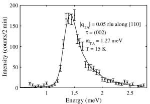
Figure 1: $\omega$-scan : TA phonon in the [110] direction ($|\vec{q}|=$ 0.05 rlu), polarized along [001]; KTaO₃, $T=$ 15 K. The fit is performed using a ’4D’ Monte Carlo convolution technique.

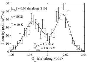
Figure 2: $q_{\perp}$-scan across a TA ’valley’ around $|\vec{q}|=$ 0.04 rlu in the [110] direction; KTaO₃, $T=10$ K. The fit is performed using a ’4D’ Monte Carlo convolution technique.

The actual fit is obtained using a least square convergence criterion implemented in a Marquardt-Levenberg gradient algorithm MFit . A typical energy scan along a principal axis is illustrated in Fig. 1. A typical off-axis wavevector scan, perpendicular to a principal direction, is shown in Fig. 2. As already remarked in Comes72 ; Perry89 , the asymmetrical line profile seen in Fig. 1, is fully accounted for by the finite wavevector resolution combined with the steep and anisotropic dispersion of the TA-mode.

3 Experimental results

3.1 Zone-center soft TO-mode

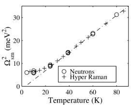
Figure 3: KTaO₃: soft TO-mode squared frequency at the zone center compared to previous hyper-Raman measurements Vogt96 . The mean energy uncertainty for the neutron data is $\Delta E\sim$ 0.1 meV.

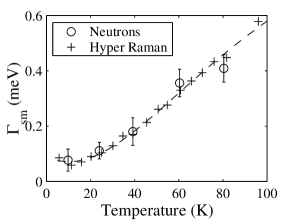
Figure 4: KTaO₃: Damping coefficient (half width) of soft zone center TO-mode compared to previous hyper-Raman measurements Vogt96 . The mean uncertainty for the neutron data is $\Delta\Gamma\sim$ 0.1 meV.

The frequency $\Omega_{sm}$ and damping $\Gamma_{sm}$ of the soft $F_{1u}$ ($\Gamma_{15}$) TO-mode at the BZ-center were obtained as a function of temperature. As shown in Fig. 3, the squared TO-frequency follows a standard Curie-Weiss law above $\sim$ 30 K, and saturates at a finite value $\Omega_{sm}^{2}\sim$ 6 meV² below 10 K. This is in perfect agreement with previous hyper-Raman determinations Inoue85 ; Vogt90 ; Vogt96 . For the mode-damping coefficient (Fig. 4), the present neutron-scattering measurements also agree perfectly with recent hyper-Raman data on a sample of similar quality Vogt96 .

3.2 Low energy phonon-dispersion curves

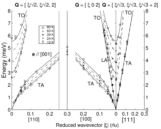
Figure 5: Dispersion curves of KTaO₃ low energy phonons between 10 and 80 K along the high symmetry axes. The mean energy uncertainty is 0.1 meV. The LA mode is measured at $\vec{Q}=[$0, 0, 2+$\xi]$. The lines correspond to calculations using the Vaks parameterization presented in this work.

Fig. 5 shows the phonon-dispersion branches measured in the high symmetry directions. These data complement the previous results from Refs. Axe70 ; Comes72 ; Perry89 . The transverse acoustic phonons measured at $\vec{Q}=[\xi,0,2]$ and $[\xi/\sqrt{2},\xi/\sqrt{2},2]$, are polarized along the [001] axis. They both correspond to the elastic constant $C_{44}$ at small $\xi$ and hence have the same dispersion over the central region of the BZ. The coupling between the TA and TO-modes lowers the acoustic phonon frequency as the TO-mode softens on decreasing $T$ Axe70 ; Perry89 . This feature affects all TA branches polarized along $<$100$>$ directions. Hence it is not seen on the TA-branch propagating in the [111] direction, nor on the TA-branch propagating along [110] and polarized along [1$\overline{1}$0] (not shown in Fig. 5).

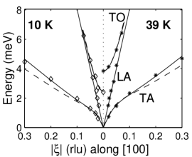
Figure 6: KTaO₃: Dispersion curves measured at 10 and 39 K in the [100] direction; the original Vaks parameterization Vaks73 is shown as dashed lines. The modified Vaks model (this work) is shown as solid lines.

The slopes of the TA-dispersion curves in the vicinity of the BZ-center are in good agreement with the elastic constants that are known from neutron and Brillouin scattering Hehlen95 ; Perry89 ; Farhi98 . In contrast to the case of the TO-mode, no measurable damping could be extracted from the TA and LA-mode experimental line-shapes. This sets an upper limit for $\Gamma_{TA}$ and $\Gamma_{LA}$ at about 0.05 meV. Finally, as seen in Fig. 6, the original Vaks model parameters Vaks73 do not describe satisfactorily low-$T$ TA-modes along high symmetry axes for $|\vec{q}|\gtrsim$ 0.1 rlu ($\omega\gtrsim$ 2 meV).

3.3 Anisotropy of the spectrum

In order to characterize the phonon-spectrum anisotropy, some off-principal axis scans were performed. Starting from a reciprocal space position on a high symmetry axis, $\vec{q}$-scans perpendicular to this axis have been performed. A typical $\vec{q}$-scan at constant $\omega$ is shown in Fig. 2. Some $\omega$-scans at constant off-axis $\vec{q}$ were also performed. Comès and Shirane first studied this anisotropy at 20 K and 300 K by mapping the LA, TA and TO-mode dispersions in the vicinity of the [100] axis. They found that the TA and TO-mode dispersions form valleys that become deeper as $T$ decreases, while the LA-mode exhibits a weak anisotropy. They ascribed the characteristic diffuse streaks observed by X-ray scattering Comes68 to the strong anisotropy of the TA-mode dispersion.

Our off-axis scans confirm this behaviour for the TA and TO-branches around the [100] and [110] directions (Figs. 7 and 8). The energy accuracy of $\sim$ 0.1 meV which is achieved on-axis deteriorates slightly as one moves away from the high symmetry direction. It is clear from Fig. 7 that the Vaks model using the original KTaO₃ parameter set Vaks73 is not satisfactory for an accurate parameterization of the dispersion surfaces away from the principal axes, even at $\vec{q}$ values as low as 0.05 rlu.

4 Parameterization of the phonon spectrum

Two alternate approaches have been used to describe the phonon spectrum of KTaO₃. First, the phenomenological description due to Vaks Vaks68 ; Vaks73 consists in expanding the lattice Hamiltonian in powers of $\vec{q}$, taking only into account the low lying phonon branches, and the interactions among them, as allowed by symmetry. The expansion, limited to the 5 lowest-energy excitations (two TA, one LA, and two TO-modes), is actually equivalent to a Ginzburg-Landau free energy expansion with respect to dielectric polarization and elastic deformations. Similar ideas have been discussed by Axe et al. Axe70 in order to account for the strong $T$-dependent depression in the TA-mode dispersion owing to the repulsion with the softening TO-mode. In the Ginzburg-Landau formalism, this effect is described as a symmetry-allowed interaction between the shear strain and the gradient of the electric polarization.

A more ambitious approach was developed by Migoni et al. Migoni76 . This is a microscopic model which aims at describing the complete phonon spectrum across the entire BZ, and which accounts for the softening of the TO-mode through the non-linear polarizability of the O^2- ion. Perry et al. Perry89 used this model to describe the phonon branches of KTaO₃ along the high symmetry directions. Their extensive neutron measurements allowed to determine the full set of 15 model parameters. However, the resolution of the experiments, and thus the accuracy of the resulting model, are not better than $\sim$0.5 meV.

At low temperatures, the thermodynamic and phonon-kinetic properties of KTaO₃ are controlled by the 5 lowest modes included in the Vaks model Vaks68 ; Vaks73 . Since our aim is not to explain the origin of the soft mode, but rather to use the phonon spectrum to account for the low temperature anomalies observed in the quantum paraelectric state, the Vaks parameterization is a very convenient one. It includes 8 adjustable parameters, but 4 of these are well determined from light-scattering data. As the physical basis of the model is only detailed in Ref. Vaks73 , we summarize it below, specializing to the cubic case which is of interest here. We shall then refine the parameter determination in order to obtain a reliable description of low-lying dispersion surfaces.

4.1 Effective Hamiltonian

One considers first the $harmonic$ part of the lattice Hamiltonian $\cal H$ of a cubic perovskite crystal. Let $\vec{u}_{i}(\vec{q})$ be the spatial Fourier transform of the displacement from equilibrium for the $i$th atom in the unit cell. The mass of this atom is denoted $m_{i}$ and its effective charge, $e_{i}$. One finds Vaks73 ; Born54 ; Kwok66

$${\cal H} = \frac{1}{2}\sum_{i,\vec{q}}m_{i}|\vec{\dot{u_{i}}}(\vec{q})|^{2}$$ (3)

$$+ \frac{1}{2}\sum_{i_{1},i_{2},\vec{q}}\vec{u}_{i_{1}}(\vec{q})\hat{\Phi}_{i_{1},i_{2}}(\vec{q})\vec{u}_{i_{2}}(-\vec{q})$$

$$- \sum_{i,\vec{q}}e_{i}\vec{u_{i}}(\vec{q})\vec{E}(-\vec{q})+\frac{\epsilon_{\infty}}{2}\sum_{\vec{q}}|E(\vec{q})|^{2},$$

where $\epsilon_{\infty}$ is the high frequency dielectric permittivity of the crystal. The tensor $\hat{\Phi}$ accounts for the ”short-range” part of the potential energy, i.e. for the contribution of the short-range forces plus the analytical (in $\vec{q}$, at $\vec{q}\rightarrow 0$) part of the dipole-dipole interaction. The non-analytical part is taken into account by introducing the Fourier transform of the macroscopic electric field $\vec{E}(\vec{q})$, which is given by Poisson’s equation,

$$\vec{q}\cdot\left[\epsilon_{\infty}\vec{E}(\vec{q})+\vec{P}(\vec{q})\right]=0\;.$$ (4)

The Fourier transform of the macroscopic electric polarization is defined by

$$\vec{P}(\vec{q})=\frac{1}{v_{c}}\sum_{i}e_{i}\vec{u_{i}}(\vec{q})\;,$$ (5)

where $v_{c}=a^{3}$ is the unit-cell volume.

Using a routine procedure, Eqs. (3), (4), and (5) give an effective Hamiltonian that can be diagonalized in terms of normal phonon coordinates. However, following Vaks Vaks68 ; Vaks73 the most convenient form of the Hamiltonian for the present purpose is obtained using a linear transformation of the displacements $\vec{u}_{i}(\vec{q})$ which diagonalizes only the short-range part of $\cal H$ in the limit $\vec{q}\rightarrow 0$. One selects a particular $\vec{u}$ to describe the acoustic modes by

$$\vec{u}_{1}(\vec{q})=\frac{1}{\sqrt{m_{1}}}\vec{u}(\vec{q})\;.$$ (6)

One defines then the optical displacements $\vec{x}_{b}(\vec{q})$ by

$$u_{i,\alpha}(\vec{q})-u_{1,\alpha}(\vec{q})=\frac{1}{\sqrt{m_{i}}}\sum_{\beta,b=1}^{4}L_{i\alpha,b\beta}x_{b,\beta}(\vec{q})\;,$$ (7)

where $\alpha$ and $\beta$ are cartesian indices. In writing (7), one takes into account that the short-range part of the lattice Hamiltonian of a cubic perovskite at small $q$ contains 4 sets of 3-fold-degenerate optic modes that correspond to the same vector irreducible representation. The subscript $b$ indexes these sets. With the new variables, Eqs. (3), (4), and (5) give:

$${\cal H} = \frac{1}{2}\sum_{\vec{q}}[\vec{\dot{u}}(-\vec{q})\vec{\dot{u}}(\vec{q})+\vec{u}(-\vec{q})\hat{A}(\vec{q})\vec{u}(\vec{q})$$ (8)

$$+ \sum_{b}\{\vec{\dot{x}}_{b}(-\vec{q})\vec{\dot{x}}_{b}(\vec{q})+\lambda_{b}\vec{x}_{b}(-\vec{q})\vec{x}_{b}(\vec{q})$$

$$+ 2\vec{u}(-\vec{q})\hat{V}_{b}(\vec{q})\vec{x}_{b}(\vec{q})\}$$

$$+ \sum_{b,b^{\prime}}\vec{x}_{b}(-\vec{q})\{\hat{S}_{b,b^{\prime}}(\vec{q})+\hat{\Phi}_{b,b^{\prime}}^{E}(\vec{q})\}\vec{x}_{b^{\prime}}(\vec{q})]\;,$$

where $\lambda_{b}$ are the restoring short-range force constants of the optic modes. The tensors $\hat{A}$, $\hat{V}_{b}$, and $\hat{S}_{b,b^{\prime}}$ correspond to the contributions of the short-range interactions. These analytically go to zero as $q^{2}$ for $\vec{q}\rightarrow 0$. The tensor $\hat{\Phi}_{b,b^{\prime}}^{E}$ is non-analytic at $\vec{q}\rightarrow 0$. It represents the contribution from the long-range part of the dipole-dipole interaction,

$$(\Phi_{b,b^{\prime}}^{E})_{\alpha\beta}=\sum_{\alpha^{\prime},\beta^{\prime}}\left(\frac{z_{b,\alpha\alpha^{\prime}}z_{b^{\prime},\beta\beta^{\prime}}}{\epsilon_{\infty}a^{3}}\right)n_{\alpha^{\prime}}n_{\beta^{\prime}},$$ (9)

where $\vec{n}=\vec{q}/|\vec{q}|$, and $z_{b,\alpha\alpha^{\prime}}=\sum_{i}e_{i}L_{i\alpha,b\alpha^{\prime}}/\sqrt{m_{i}}$ is the effective charge tensor for the $b$-set of optic modes in the limit $\vec{q}\rightarrow 0$, which in view of the cubic symmetry is $\propto\delta_{\alpha\alpha^{\prime}}$ Vaks73 .

One is only interested in the low frequency part of the spectrum. Following Vaks Vaks68 ; Vaks73 , one first diagonalizes the optical part of (8) in the limit $\vec{q}\rightarrow 0$, keeping only the terms containing the restoring short-range force constants of the optic modes , $\lambda_{b}$, and the non-analytical term $\hat{\Phi}_{b,b^{\prime}}^{E}$. One finds that the latter lifts the degeneracy of the optical modes, splitting each set into a pair of degenerate TO-modes, whose frequency squared is equal to $\lambda_{b}$, and a longitudinal (LO) mode. One pair of TO-modes in the set $b$ corresponds to the soft mode, which has a frequency $\Omega_{sm}$ much lower than all other optic modes. It is associated to the hardest LO mode Zhong94 , labelled LO₄ in the Perry et al. denomination Perry89 . We denote the corresponding $\lambda_{b}$ by $\lambda$ and the corresponding optical displacement vector $\vec{x}_{b}$ by $\vec{x}$. The anharmonic interactions, not included in 3, are taken into account with a standard quasi-harmonic approximation. The frequency of the soft mode becomes then temperature dependent through the $T$-dependence of $\lambda=\Omega^{2}_{sm}$. In futher considerations, only the subset consisting of the two soft TO-modes and of the 3 acoustic modes is kept. One neglects the other optical modes as well as their interactions with this subset. As shown by Vaks Vaks68 ; Vaks73 , the accuracy of this approximation for the description of a phonon of frequency $\omega$ is controlled by the small parameter ${\omega^{2}}/{\Omega^{2}_{op}}$, where $\Omega_{op}$ is a typical hard optical mode frequency such as the hard LO₄ mode. Hence for the part of the spectrum that we are interested in ($\omega\simeq\Omega_{sm}$), it results from the Lyddane-Sachs-Teller relation that this parameter is of order $\epsilon_{\infty}/\epsilon_{o}$, where $\epsilon_{o}$ is the static dielectric permittivity of the crystal.

Technically, the separation of the Hamiltonian containing only the 5 modes of interest is done to within the aforementioned accuracy by considering the problem in a rotated reference frame $\vec{X^{\prime}}\equiv(X^{\prime}_{1},X^{\prime}_{2},X^{\prime}_{3})$, rather than in the usual cubic frame $\vec{X}\equiv(X_{1},X_{2},X_{3})$. The axis $X^{\prime}_{3}$ is taken parallel to $\vec{q}$. Specifically, the rotated frame can be defined by the relation $\vec{X}^{\prime}=\hat{M}\vec{X}$, where the matrix $\hat{M}$ is given as a function of the direction of $\vec{q}$ ($\vec{n}=\vec{q}/q$) by

$$M(\vec{n})=\left(\begin{array}[]{ccc}0&n_{\perp}&n_{1}\\ -n_{3}/n_{\perp}&-n_{1}n_{2}/n_{\perp}&n_{2}\\ n_{2}/n_{\perp}&-n_{1}n_{3}/n_{\perp}&n_{3}\end{array}\right),$$ (13)

where $\vec{n}$ is written in the cubic reference frame $\vec{X}$, and $n_{\perp}^{2}=1-n_{1}^{2}$.

One sees that in the rotated frame the components of the acoustic and optical bare mode displacements (as defined in (6) and (7)), associated with the 5 modes of interest are just $x_{1},x_{2},u_{1},u_{2}$, and $u_{3}$, while $x_{3}$ is essentially the displacement of the LO₄ mode which has been eliminated. Finally, the 5-mode Hamiltonian can be written Vaks68 ; Vaks73 :

$${\cal H}^{(5)} = \frac{1}{2}\sum_{\vec{q}}[\dot{\vec{u}}_{-q}\dot{\vec{u}}_{q}+\vec{u}_{-q}{\hat{A}}(\vec{q})\vec{u}_{q}+\dot{\vec{x}}_{-q}\dot{\vec{x}}_{q}$$

$$+ \lambda\vec{x}_{-q}\vec{x}_{q}+\vec{x}_{-q}{\hat{S}}(\vec{q})\vec{x}_{q}$$

$$+ 2\vec{u}_{-q}\hat{V}(\vec{q})\vec{x}_{q}]\;.$$

The components of the tensors $\hat{A}$, $\hat{S}$ and $\hat{V}$ that give non-vanishing contributions in the subspace ($x_{1},x_{2},u_{1},u_{2},u_{3}$) in the small-$q$ limit are

$$\hat{A} = q^{2}(A_{l}g^{l}+A_{t}g^{t}+A_{a}g^{a}),$$

$$\hat{S} = q^{2}(S_{t}g^{t}+S_{a}g^{a}),$$ (15)

$$\hat{V} = q^{2}(V_{t}g^{t}+V_{a}g^{a}),$$

with

$$g^{l}_{\alpha\beta} = n_{\alpha}n_{\beta},$$

$$g^{t}_{\alpha\beta} = \delta_{\alpha\beta}-n_{\alpha}n_{\beta},$$ (16)

$$g^{a}_{\alpha\beta} = \gamma_{\alpha\beta\gamma\delta}n_{\gamma}n_{\delta}.$$

The tensor $\gamma_{\alpha\beta\gamma\delta}$ is defined, in the cubic frame, by $\gamma_{\alpha\beta\gamma\delta}=1$ if $\alpha=\beta=\gamma=\delta$, and $\gamma_{\alpha\beta\gamma\delta}=0$ otherwise. In that frame, $\hat{A}$, $\hat{S}$, and $\hat{V}$ stand for acoustic, optic, and acoustic-optic coupling tensors respectively, split into transverse $g^{t}$, longitudinal $g^{l}$, and anisotropic $g^{a}$ parts, as seen in (4.1). The coefficients $S_{l}$ and $V_{l}$ do not appear in (4.1) since $\vec{x}$ is taken as purely transverse.

Since the kinetic energy terms are already diagonal, the phonon-dispersion curves for the 5 branches are given by the square roots of the eigenvalues of the following matrix:

$${\cal H}^{(5)}(\vec{q}) = {\cal H}_{is}(|\vec{q}|,\lambda,S_{t},A_{t},V_{t},A_{l})$$ (17)

$$+ {\cal H}_{anis}(\vec{q},S_{a},A_{a},V_{a})\;.$$

The isotropic matrix, ${\cal H}_{is}$, is

$$\left(\begin{array}[]{ccccc}\lambda+S_{t}q^{2}&0&V_{t}q^{2}&0&0\\ 0&\lambda+S_{t}q^{2}&0&V_{t}q^{2}&0\\ V_{t}q^{2}&0&A_{t}q^{2}&0&0\\ 0&V_{t}q^{2}&0&A_{t}q^{2}&0\\ 0&0&0&0&A_{l}q^{2}\end{array}\right),$$ (23)

and the anisotropic one, ${\cal H}_{anis}$, is

$$q^{2}\left(\begin{array}[]{ccccc}S_{a}h_{11}&S_{a}h_{12}&V_{a}h_{11}&V_{a}h_{12}&V_{a}h_{13}\\ S_{a}h_{12}&S_{a}h_{22}&V_{a}h_{12}&V_{a}h_{22}&V_{a}h_{23}\\ V_{a}h_{11}&V_{a}h_{12}&A_{a}h_{11}&A_{a}h_{12}&A_{a}h_{13}\\ V_{a}h_{12}&V_{a}h_{22}&A_{a}h_{12}&A_{a}h_{22}&A_{a}h_{23}\\ V_{a}h_{13}&V_{a}h_{23}&A_{a}h_{13}&A_{a}h_{23}&A_{a}h_{33}\end{array}\right),$$ (29)

in which

$$\begin{array}[]{lll}h_{11}&=&\frac{2n_{2}^{2}n_{3}^{2}}{n_{\perp}^{2}}\;,\\ h_{12}&=&\frac{n_{1}n_{2}n_{3}}{n_{\perp}^{2}}(n_{3}^{2}-n_{2}^{2})\;,\\ h_{22}&=&2n_{1}^{2}(n_{\perp}^{2}-\frac{n_{2}^{2}n_{3}^{2}}{n_{\perp}^{2}})\;,\\ \end{array}\begin{array}[]{lll}h_{13}&=&\frac{n_{2}n_{3}}{n_{\perp}}(n_{2}^{2}-n_{3}^{2})\;,\\ h_{23}&=&\frac{n_{1}}{n_{\perp}}(n_{1}^{2}n_{\perp}^{2}-n_{2}^{4}-n_{3}^{4})\;,\\ h_{33}&=&n_{1}^{4}+n_{2}^{4}+n_{3}^{4}\;.\end{array}$$

The eigenvalues $\omega_{i}(\vec{q})$ of ${\cal H}^{(5)}(\vec{q})$ are the squared phonon frequencies, and the diagonalization matrix $L_{i,j}(\vec{q})$ reflects the mode mixing. Thus, the renormalized acoustic $\vec{u}$ and optical $\vec{x}$ displacements in the canonical cubic axis system are obtained through a linear combination of bare mode displacements:

$$\vec{x}_{j,\vec{q}}=\sum_{j^{\prime}_{opt}=1,2}\vec{M}_{j^{\prime}}L_{j,\vec{q}}^{(j^{\prime})}\mbox{ and }\vec{u}_{j,\vec{q}}=\sum_{j^{\prime}_{ac}=3,4,5}\vec{M}_{j^{\prime}-2}L_{j,\vec{q}}^{(j^{\prime})},$$ (32)

where $\vec{M}_{j}$ indicates the column $j$ in matrix $M$.

In the matrix ${\cal H}_{is}$, the parameters $S_{t}$, $A_{t}$, and $A_{l}$ appear as squared dispersion-curve slopes whereas $V_{t}$ is a TA-TO coupling parameter, and $S_{a}$, $A_{a}$, and $V_{a}$ contribute to the off-principal axis squared slopes.

4.2 Adjustment of the phonon-dispersion surfaces

We now use the above model to parameterize the measured phonon spectra. Since the parameter set given by Vaks for KTaO₃ (see Table 1 and Figures 6 and 7) leads to typical deviations of 0.5 meV or more with respect to our inelastic neutron scattering measurements, it is necessary to recompute the parameter values. The model contains 8 parameters: $S_{t}$, $A_{t}$, $V_{t}$, $S_{a}$, $A_{a}$, $V_{a}$, $A_{l}$, and $\lambda=\Omega_{sm}^{2}$, where only the latter is appreciably $T$-dependent. Three parameters can be expressed in terms of the elastic constants $C_{ij}$ and the density $\rho=6.967$ g/cm³ of the crystal Vaks68 ; Vaks73 :

$$A_{l} = (C_{12}+2C_{44})/{\rho}\;,$$

$$A_{t} = C_{44}/{\rho}\;,$$ (33)

$$A_{a} = (C_{11}-C_{12}-2C_{44})/{\rho}\;.$$

The values of the elastic constants are known from Brillouin-scattering experiments Hehlen95 ; Farhi98 : $C_{11}=4.344\pm 0.049$, $C_{12}=1.027\pm 0.038$, and $C_{44}=0.990\pm 0.020$ in 10¹¹ N/m². The $T$-dependent values of $\lambda$ are available from the hyper-Raman measurements Inoue85 ; Vogt90 ; Vogt96 . The values used presently are given in Table 2. Thus, there remain only 4 adjustable parameters at our disposal, namely $S_{t}$, $V_{t}$, $S_{a}$, and $V_{a}$. We adjusted our data on the 5 lowest frequency modes for the $<$100$>$, $<$110$>$, and $<$111$>$ directions to the square roots of the eigenvalues of the matrix (17). The fit was performed with a Marquadt-Levenberg algorithm and a least square criterion, for the temperatures, 10, 24, 39, 60, and 80 K, keeping the parameters temperature independent. The overall correlation coefficient when using 151 neutron and Brillouin measurements is $r^{2}=0.995$, and the determined model parameters are given in Table 1. This table also contains the sets of parameters determined by previous workers Axe70 ; Vaks68 ; Vaks73 . Appreciable differences in some of these can be seen. The obtained parameterization of the spectrum has been tested by comparing the phonon frequencies measured off principal directions with those calculated from the parameters, as shown in Figs.7 and 8. One sees that the model gives also a reasonable description for the off-axis dispersion.

The model provides a global description of the low-frequency spectrum of KTaO₃ as illustrated in Fig. 9 and 10. A remarkable feature of the phonon spectrum is the strong anisotropy of the TO and TA modes. We conclude that the Vaks model provides a very reasonable parameterization of the five lowest phonon modes of KTaO₃ ($\omega<8$ meV) in the central part of the Brillouin zone ($|\vec{q}|<0.25$ rlu) and in the low temperature region ($10<T<100$ K). The achieved accuracy is $\sim 0.1$ meV in the vicinity of the high symmetry axes, and remains better than $\sim$ 0.2-0.3 meV away from these i.e. of the order of the experimental uncertainties.

5 Conclusion

We presented the results of cold neutron high resolution inelastic scattering measurements of KTaO₃ at low temperatures, for the lowest phonon-dispersion branches and for wave vectors $|\vec{q}|<0.25$ rlu. A Monte-Carlo convolution technique based on a modelisation of the 4-dimensional resolution ellipsoid was used in order to extract phonon frequencies and dampings from the experimental spectra. The present results improve significantly on previous phonon studies in KTaO₃ at low-$T$ Axe70 ; Shirane67 ; Harada70 ; Comes72 ; Perry89 . In particular, the accuracy on the phonon frequencies if of the order of 0.1 meV along symmetry directions and it appears to remain better than 0.3 meV in non-symmetry directions. The phenomenological model by Vaks Vaks68 ; Vaks73 , which contains 8 parameters (4 of them being determined from light-scattering experiments) was used for the parameterization of the low-energy phonon spectrum. By adjusting 4 temperature-independent parameters an accurate description of the spectrum was achieved over the temperature range from 10 to 100 K.

The relatively simple description of the temperature-dependent spectrum of KTaO₃ which is thus obtained provides a convenient basis for quantitative calculations of all the properties that are controlled by the low frequency phonons. In particular it becomes possible to calculate thermodynamic and transport properties at low temperatures, such as phonon-density-fluctuation processes and second sound, in the low-$T$ quantum paraelectric regime. Such calculations will be the object of a forthcoming publication.

The authors thank Alain Brochier for his efficient technical support during the IN14 experiments at ILL.

$(meV/rlu)^{2}$	$S_{t}$	$A_{t}$	$V_{t}$	$S_{a}$	$A_{a}$	$V_{a}$	$A_{l}$
Ref. Balagurov70 ; Vaks73	4860	1836	2808	10800	2160	-5724	4320
Ref. Axe70	4670	1830	2800
This work	4828	1553	2451	8956	2265	-3087	4552
(uncertainty)	(20)	(10)	(30)	(400)	(40)	(290)	(30)

Table 1: Low temperature Vaks parameters of KTaO₃, determined from a global fit of neutron and Brillouin data. See Sec. 4.1 for the meaning of the parameters.

$T$ (K)	80	60	39	24	10
$\lambda$ (meV)2	30.8	23.1	14.9	9.2	6.2
(uncertainty)	(0.5)	(0.8)	(0.5)	(0.4)	(0.3)

Table 2: Square of the soft mode frequency, $\lambda$, used in our refined Vaks parameterization.

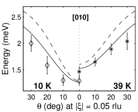
Figure 7: Measured dispersion curves in KTaO₃ at 10 and 39 K near the [010] direction in the (001) scattering plane: $\vec{Q}$ = [(2+$\xi\sin\theta$), ($\xi\cos\theta$), 0]; The dashed and solid lines refer to the original Vaks73 and modified (this work) Vaks parameters.

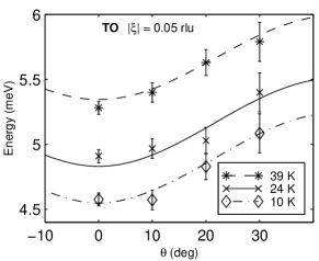
Figure 8: Anisotropy of the TO phonon branch near the [010] symmetry axis in KTaO₃: $\vec{Q}$ = [(2+$\xi\sin\theta$), ($\xi\cos\theta$), 0]. The lines are calculated with the modified Vaks parameters.

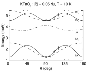
Figure 9: KTaO₃: The low frequency phonon spectrum at $T=$ 10 K, for $\vec{q}$ = [($\xi\sin\theta$), ($\xi\cos\theta/\sqrt{2}$), ($\xi\cos\theta/\sqrt{2}$)] with $|\vec{\xi}|=$ 0.05 rlu, as computed by our Vaks-type parameterization. The directions [110], [111] and [001] correspond to the angles 0^∘ or 180^∘, 35.3^∘ or 144.8^∘, and 90^∘, respectively. The experimental data points are shown as open circle.

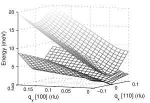
Figure 10: Highly anisotropic coupled acoustic and optical phonon surfaces at $T=$ 10 K in KTaO₃ showing a deep valley around the [100] direction; calculated from the modified Vaks parameters.

References

- (1) K. Kurtz, Trans. Am. Cryst. Assoc. 2, (1975) 63.
- (2) K.A. Müller and H. Burkard, Phys. Rev. B 19, (1979) 3593.
- (3) J.D. Axe, J. Harada, and G. Shirane, Phys. Rev. B 1, (1970) 1227.
- (4) B. Hehlen, L. Arzel, A.K. Tagantsev, E. Courtens, Y. Inaba, A. Yamanaka, and K. Inoue, Phys. Rev. B 57, (1998) R13989.
- (5) B. Hehlen, A-L. Pérou, E. Courtens, and R. Vacher, Phys. Rev. Lett. 75, (1995) 2416.
- (6) B. Hehlen, Doctoral thesis, Université de Montpellier II (1995).
- (7) E. Courtens, B. Hehlen, G. Coddens, B. Hennion, Physica B : Cond. Matt. 219, (1996) 577.
- (8) K.B. Lyons and P.A. Fleury, Phys. Rev. Lett. 37, (1976) 161.
- (9) H. Unoki and T. Sakudo, J. Phys. Soc. Jap.23, (1967) 546.
- (10) H. Thomas and K.A. Müller, Phys. Rev. Lett.21, (1968) 1256.
- (11) G. Shirane and Y. Yamada, Phys. Rev. 177, (1969) 858.
- (12) J. Feder and E. Pytte, Phys. Rev. B 1, (1970) 4803, and refs. therein.
- (13) L. Arzel, B. Hehlen, R. Currat, B. Hennion, M. Saint-Paul, and E. Courtens, Ferroelectrics, to be published in the Proceedings of EMF-9, Prague (1999).
- (14) P.A. Fleury and J.M. Worlock, Phys. Rev. Lett. 18, (1967) 665.
- (15) K. Inoue, Jap. J. App. Phys. 24, (1985) 107.
- (16) H. Vogt, Phys. Rev. B 41, (1990) 1184.
- (17) G. Shirane, R. Nathans, and V.J. Minkiewicz, Phys. Rev. 157, (1967) 396.
- (18) J. Harada, J.D. Axe, and G. Shirane, Acta. Cryst. A26, (1970) 608.
- (19) R. Comès and G. Shirane, Phys. Rev. B 5, (1972) 1886.
- (20) C.H. Perry, R. Currat, H. Buhay, R.M. Migoni, W.G. Stirling, and J.D. Axe, Phys. Rev. B 39, (1989) 8666.
- (21) P. Grenier, G. Bernier, S. Jandl, B. Salce, and L.A. Boatner, J. Phys. : Cond. Matt. 1, (1989) 2515.
- (22) S. Jandl, M. Banville, P. Dufour, S. Coulombe, and L.A. Boatner, Phys. Rev. B 43, (1991) 7555.
- (23) D. Rytz, U.T. Höchli, and H. Bilz, Phys. Rev. B 22, (1980) 359.
- (24) B. Salce, J.L. Gravil, and L.A. Boatner, J. Phys. : Cond. Matt. 6, (1994) 4077.
- (25) R. Migoni, H. Bilz, and D. Bäuerle, Phys. Rev. Lett. 25, (1976) 1155.
- (26) H. Bilz, G. Benedek, and A. Bussmann-Holder, Phys. Rev. B 35, (1987) 4840.
- (27) V.G. Vaks, Zh. Eksp. Teor. Fiz. 54, (1968) 910 [Sov. Phys. JETP 27, (1968) 486].
- (28) V.G. Vaks, Vvedenie v Mikroskopicheskuyu Teoriyu Segnetoelectrikov [Introduction to the Microscopic Theory of Ferroelectrics], Nauka, Moscow (1973).
- (29) J. Toulouse and B. Hennion, Phys. Rev. B 49, (1994) 1503.
- (30) K.S. Klein, G.E. Kugel, and B. Hennion, J. Phys.: Condens. Matter 8 (1996) 1109.
- (31) M.D. Fontana, G.E. Kugel, L. Foussadier, W. Kress, and D. Rytz, Europhys. Lett. 23, (1993) 427.
- (32) L. Foussadier, M.D. Fontana, and W. Kress, J. Phys.: Condens. Matter 8, (1996) 1135.
- (33) E. Farhi, A.K. Tagantsev, B. Hehlen, R. Currat, L.A. Boatner, and E.Courtens, Ferroelectrics, EMF9 Proceedings, to be published (1999). See also E. Farhi et al., Physica B, ECNS99 Proceedings, to be published (1999).
- (34) E. Farhi, Doctoral thesis, Université Montpellier II (1998). http://www.ill.fr/tas/Farhi.html
- (35) J.R. Thomson, L.A. Boatner, and J.O. Thomson, J. Low Temp. Physics, 47, (1982) 5.
- (36) M. Popovici, Acta Cryst. A31, (1975) 507.
- (37) D.A. Tennant and D. McMorrow, Rescal v5.1, a Matlab(R) tool for 3-axis neutron-scattering-resolution calculation (1996). http://www.ill.fr/tas/matlab/doc/matprgs.html
- (38) B. Fåk and B. Dorner, Physica B 234, (1997) 1107.
- (39) D.A. Tennant, D. McMorrow, M.Zinkin and E. Farhi, MFit v4.2, a Matlab(R) tool for curve analysis and fitting (1998).
- (40) H. Vogt, Ferroelectrics 184, (1996) 31.
- (41) R. Comès et al, Sol. State Comm. 6, (1968) 715.
- (42) M. Born and K. Huang, Dynamical theory of crystal lattices, Oxford University Press (1954).
- (43) P.C. Kwok and P.B. Miller, Phys. Rev. B 151, (1966) 387.
- (44) W. Zhong, R.D. King-Smith, and D. Vanderbilt, Phys. Rev. Lett. 72, 3618 (1994).
- (45) B.Y. Balagurov, V.G. Vaks and B.I. Shklovshii, Fiz. Tverd. Tela 12, (1970) 89 [Sov. Phys. Solid State 12, (1970) 70].