Dynamic Scaling in Diluted Systems Phase Transitions: Deactivation trough Thermal Dilution

Abstract

Activated scaling is confirmed to hold in transverse field induced phase transitions of randomly diluted Ising systems. Quantum Monte Carlo calculations have been made not just at the percolation threshold but well bellow and above it including the Griffiths-McCoy phase. A novel deactivation phenomena in the Griffiths-McCoy phase is observed using a thermal (in contrast to random) dilution of the system

The presence of quenched disorder in quantum phase transitions at zero temperature is a topic of current interest. Two of the most important special properties of the disordered quantum phase transitions are the appearance of activated dynamic scaling and the existence of Griffiths-McCoy singularities [1, 2] even away from the critical point.

Activated dynamic scaling was first analytically proved to hold in the disordered one dimensional Ising model in a transverse field [3] and there are many other results for this model in the literature [4, 5, 6, 7, 8]. The disordered Ising model in a transverse field considered as a quantum spin glass provides a reasonable description of the system $LiHo_{x}Y_{1-x}F_{4}$ [9] and also, considering the existence of long-range correlated disorder in it, may be an appropriate model to describe non-Fermi liquid behavior in certain $f$-electron systems [10, 11, 12]. Activated dynamic scaling implies the existence of an infinite dynamic critical exponent $(z=\infty$). It means that instead of the typical power law relationship between the characteristic time scale and the characteristic length scale, $\xi_{\tau}\sim\xi^{z},$ a new exponential relation appears $\xi_{\tau}\sim exp(const\times\xi^{\psi})$ with $\psi=1/2$ for the one-dimensional Ising model [3]. There are nearly no analytical results for higher dimensions. The activated dynamic scaling seems to disappear for two-dimensional [13] and three dimensional Ising glass systems [14], but it has been proved to hold in the disordered two-dimensional Ising model in a transverse field by means of Quantum Monte Carlo simulations [15, 16] and renormalization group analysis [17]. The only analytical prediction of activated scaling in dimensions higher than one has been made for the dilution probability transition at the percolation threshold $(p_{c})$ of a diluted Ising system in a transverse field [18], where percolation critical exponents have been found.

The phase boundary of this model at $T=0$ was studied a long time ago [19, 20, 21] and is expected to have a multi-critical point and a straight vertical phase boundary separating the ferromagnetic phase from the quantum Griffiths phase at the percolation threshold. The existence of this boundary and the activated scaling predicted by Senthil et al. has been recently checked by means of Quantum Monte Carlo simulations, comparing the dilution probability transitions at constant transverse fields for $p$ values bellow an above the one corresponding to the multicritical point[22].

However, there is no study of the existence of activated scaling for transitions tuned by the transverse field in diluted Ising systems. These systems present a great advantage: fixing the probability of occupied places $(p)$ and varying de transverse field $(\Gamma)$ at $T=0,$ it is possible to follow the evolution of the activated scaling at zero temperature in the ferromagnetic phase $(p>p_{c})$ at the phase boundary $(p=p_{c})$ and in the Griffiths phase $(p<p_{c})$. In this paper we will use the diluted Ising model in a transverse field to directly determine the existence and evolution of activated scaling in the three different zones of the phase diagram. We will show how the activated scaling exists not just at the percolation threshold but well above it and how it reaches a maximum near the phase boundary $(p=p_{c}$) keeping mostly constant all the way through the Griffiths zone. We start from the two-dimensional $(d=2)$ diluted Ising model in a transverse field with Hamiltonian given by

$${\cal H}=-\sum\limits_{\left\langle i,j\right\rangle}\varepsilon_{i}\varepsilon_{j}\sigma_{i}^{z}\sigma_{j}^{z}-\Gamma\sum\limits_{i}\varepsilon_{i}\sigma_{i}^{x}$$ (1)

where $\varepsilon_{i}\in\left\{0,1\right\}$ are quenched random variables producing the dilution. $\varepsilon_{i}=1$ with probability $p$ and $\varepsilon_{i}=0$ with probability $1-p$. In order to perform the Monte Carlo calculations we use the Suzuki-Trotter decomposition [23] and we map the phase transition at $T=0$ of the two-dimensional quantum system in a three dimensional classical system with action

$${\cal S}=-K_{hor}\sum\limits_{\tau,\left\langle i,j\right\rangle}\varepsilon_{i}\varepsilon_{j}s_{i}(\tau)s_{j}(\tau)-K_{ver}\sum\limits_{\tau,i}\varepsilon_{i}s_{i}(\tau)s_{i}(\tau+1)$$ (2)

with $K_{hor}=\Delta\tau$, $K_{ver}=-(1/2)ln\left[tanh(\Delta\tau\Gamma)\right]$ and $\Delta\tau\rightarrow 0$. This limit may be taken into account exactly considering a continuous time algorithm [16], however making use of the universality between the model with $\Delta\tau\rightarrow 0$ and the model with $\Delta\tau\neq 0$, we may simulate the usual discrete Ising model, but with anisotropic interactions. In order to avoid problems arising from de critical slowing down at the critical point we use the Wolff single cluster algorithm [24]. It is important to notice that once an spin is diluted, the whole imaginary time axis (Trotter axis) is also diluted, which means that the random disorder in a quantum system is equivalent to the long range correlated disorder in classical systems [25] giving rise to a different universality class. In order to obtain the $T=0$ phase boundary we fix the occupied site probability $(p)$ and we consider different values of the transverse field $(\Gamma)$ at intervals of $\Delta\Gamma=0.02$. We really do not fix the probability but the concentration, it means that we do not use a grand canonical distribution of the vacancies but a canonical distribution, however both kinds of constrains are supposed to belong to the same universality class [26].

The critical magnetic field for each probability $\Gamma(p)$ is determined by a method previously used for Ising spin glasses [13, 14]. First it is necessary to compute the Binder Cumulant average from a certain number of realizations of the disorder (in our case we consider $500$ different realizations), this is done for a fixed value of ($\Gamma,p)$ and for a fixed value of the size (we consider the values $L=8,12,16,24$). Then we study the evolution of such a cumulant for different sizes of the Trotter axis (we consider up to $L_{\tau}=600$). Due to the dynamic scaling form of the Binder Cumulant it has a peak as a function of $L_{\tau}$. At the critical point ($\Gamma_{c}(p))$ the peak height is independent of $L$ and the values of $L_{\tau}$ at the maximum, $(L_{\tau})_{m}$, vary as $L^{z}$ for conventional dynamic scaling and like $(L_{\tau})_{m}\sim exp(const\times L^{\psi})$ for activated scaling. Of course, all the non-universal quantities, as for example the critical values of the transverse field, will depend on the model and in particular on $\Delta\tau$. In the present work we choose $\Delta\tau=1/5$.

The results for the phase boundary at $T=0$ are shown in Fig.1 together with the phase boundary obtained for the classical system by means of conventional scaling. The points where the existence of activated scaling is going to be checked are $p=1$ (pure case), $p=0.8,0.7$ ($p>p_{c}$), $p=0.6\simeq p_{c}\simeq 0.59$ [27] and $p=0.55,0.5$ ($p<p_{c}$) (Griffiths phase). The results for $(L_{\tau})_{m}$ vs. $L$ are presented in Fig.2. Note how the scaling is not activated for the pure case $(p=1)$ where the dynamical exponent is found to be $z\approx 1$, but it starts to activate as the dilution is increased. To ensure that for diluted cases the scaling is activated Fig.3 presents a plot of $ln(L_{\tau})_{m}$ vs. $L$. The straight line behavior for the values $p\neq 1$ clearly indicates that the scaling is activated. The evolution of the values $\psi(p)$ is presented in the inset. Note how it grows monotonically until $p\simeq p_{c}$ and then it keeps approximately constant inside the Griffiths zone.

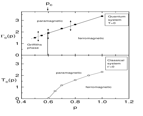
FIG. 1.: Phase diagram calculated for the classical model, $T_{c}$ vs. $p$ (white points) and for the quantum model at $T=0$, $\Gamma_{c}$ vs. $p$ (black points). Solid lines are a guide for the eye. Dotted line indicates the phase boundary in the Griffiths region ($p<p_{c}$). The three arrows indicate the transitions to study, above the percolation thershold, at the percolation thershold, and inside the Griffiths zone.

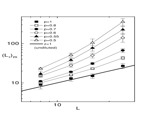
FIG. 2.: $(L_{\tau})_{m}$ vs. $L$ for different values of the spin concentration. Thin straight lines are just a guide for the eye. Thick line represents the behavior expected for the pure system ($z=1$).

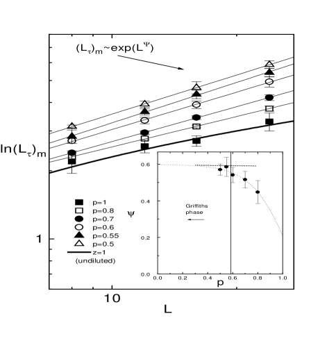
FIG. 3.: $ln(L_{\tau})_{m}$ vs. $L$ for different values of the spin concentration. Thin lines are the linear fittings and the thick line is the behavior expected for the pure system ($z=1$). Inset shows the behavior of the exponent $\psi(p)$. Dotted line is a sigmoidal fitting.

So, basically, the results presented indicate that the scaling is activated not just near the percolation threshold but well above it, and that it keeps nearly constant when the transition considered is inside of the Griffiths-McCoy quantum zone, at least for the values of $p$ considered, which are near $p_{c}$ (it may be also a maximum). Note that we are using, up to now, a purely random procedure to produce the diluted samples.

The existence of the Griffiths-McCoy zone is due to rare regions which are locally in the wrong phase. Basically there are some strongly coupled regions or clusters in the ferromagnetic phase even for spin concentrations smaller than the percolation threshold of the system. This zones are found studying the tail of local susceptibilities [7, 28, 29, 30, 31, 32, 33]. The quantum transitions allow the existence of these clusters in the wrong phase but they are very difficult to detect in classical systems. As we have shown the phase transitions (tuned by the transverse field) due to these rare regions also present activated scaling.

However there might be a possible way to deactivate the scaling in the Griffiths zone. Using the Suzuki-Trotter formalism the existence of the wrong phase comes from clusters which are infinite in the imaginary time direction, but they still are finite in the perpendicular slices. That is the reason why is possible to ”feel” the effect of the dilution by the existence of an activated scaling. However, if the dilution is not introduced randomly, but incorporating an infinite correlation length between spins and vacancies some of the clusters formed in the slices may be considered to have infinite size. The wrong phase arising in these clusters is equivalent to the pure system ordered phase and is not affected by disorder. In this case the system in the Griffiths zone is expected to show deactivated scaling. Of course, this will happen just if the phase transition is due to the existence of strongly coupled regions (i.e. if the system is in the Griffiths phase $(p<p_{c})$), but if the magnetic response is due to whole system (i.e. $p>p_{c}$) the introduction of long range correlated disorder will affect changing the universality class of the system (as in thermal classic transitions [25]) and enhancing the activation of the scaling [12].

A way to produce this kind of dilution is using the thermal dilution instead of a random dilution [34]. With this kind of dilution the system belongs to the universality class of long-range correlated disordered systems with an exponent $a=2-\eta$ [35], being $\eta$ equal to $0.25$ for the classical ($d=2)$ Ising model (the way to produce thermal dilution is described in [34]). Basically the procedure is as follows, the pure system is first thermalized to criticality and then one kind of spins are turned into vacancies. The samples produced by thermal dilution at criticality will have an spin concentration near $p=0.5$, so we can compare them only with samples diluted randomly with probability $p=0.5$. Both kinds of dilution will be at the Griffiths phase since in both cases $p_{c}(a)>0.5$ [36].

The analysis performed has been exactly the same as before but now going up to $L=40$. By the Binder Cumulant we have been able to determine the critical transverse magnetic field ($\Gamma_{c}(thermal)\simeq 3.13$) and the relation between $(L_{\tau})_{m}$ and $L$. Fig.4 compares de behavior of the thermal dilution with the behavior of the random dilution with $p=0.5$. The thick line represents the pure behavior (excepting proportional factors). Clearly the scaling has been deactivated, as expected, and $z\simeq 1$ as corresponds to the behavior of the pure system. This phenomenon could never happen with a system away from the quantum Griffiths zone.

In conclusion, Quantum Monte Carlo calculations in diluted Ising models in a transverse field at $T=0$ show that dynamic scaling holds above the percolation threshold $(p>p_{c})$, at the percolation threshold $(p=p_{c})$ and inside the quantum Griffiths-McCoy phase $(p<p_{c})$. The evolution of the activated scaling has been characterized, showing how it grows monotonously towards the value corresponding to the percolation threshold and how it appears to remain nearly constant in the Griffiths zone for values of $p$ near $p_{c}$. A new way to deactivate the scaling in the Griffiths zone by thermal dilution has been proposed. The expected deactivation works due to the fact that phase transitions come from strongly coupled regions, and not from the whole sample. The deactivation has been clearly confirmed by means of Quantum Monte Carlo simulations.

We thank P. A. Serena for generous access to his computing facilities. Financial support from DGCyT through grant PB96-0037 is gratefully acknowledged.

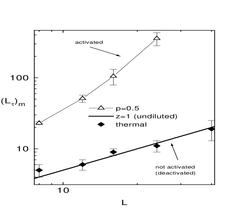
FIG. 4.: $(L_{\tau})_{m}$ vs. $L$ for a randomly diluted system with spin concentration $p=0.5$ and a thermally diluted system. The thin line is a guide for the eye, and the thick line represents the behavior expected for the pure case ($z=1$) excepting proportional factors. Note how the scaling has been deactivated for the thermal case.

REFERENCES

- [1] R. B. Griffiths, Phys. Rev. Lett. 23, 17 (1969).
- [2] B. M. McCoy, Phys. Rev. Lett. 23, 383 (1969); Phys. Rev. 188, 1014 (1969).
- [3] D. S. Fisher, Phys. Rev. Lett. 69, 534 (1992); Phys. Rev. B 51, 6411 (1995).
- [4] R. Shankar and G. Murthy, Phys. Rev. B 36, 536 (1987).
- [5] B. M. McCoy and T. T. Wu, Phys. Rev. 176, 631 (1968); 188, 982 (1969).
- [6] R. H. McKenzie, Phys. Rev. Lett. 77, 4804 (1996).
- [7] F. Iglói and H. Rieger, Phys. Rev. B 57, 11404 (1998).
- [8] A. P. Young, Phys. Rev. B 56, 11691 (1997).
- [9] W. Wu, B. Bitko, T. F. Rosenbaum and G. Aeppli, Phys. Rev. Lett. 71, 1919 (1993).
- [10] A. H. Castro Neto, G. Castilla and B. A. Jones, Phys. Rev. Lett. 81, 3531 (1998).
- [11] M. C. de Andrade, R. Chan, R. P. Dickey, N. R. Dilley, E. J. Freeman, D. A. Gajewski and M. B. Maple, Phys. Rev. Lett. 81, 5620 (1998).
- [12] H. Rieger and F. Iglói, Phys. Rev. Lett. 83, 3741 (1999).
- [13] H. Rieger and A. P. Young, Phys. Rev. Lett. 72, 4141 (1994).
- [14] M. Guo, R. N. Bhatt and D. A. Huse, Phys. Rev. Lett. 72, 4137 (1994).
- [15] C. Pich, A. P. Young, H. Rieger and N. Kawashima, Phys. Rev. Lett. 81, 5916 (1998).
- [16] H. Rieger and N. Kawashima, Eur. Phys. J. B 9, 233 (1999).
- [17] O. Motrunich, S. -C. Mau, D. A. Huse and D. S. Fisher, Phys. Rev. B 61, 1160 (2000).
- [18] T. Senthil and S. Sachdev, Phys. Rev. Lett. 77, 5292 (1996).
- [19] A. B. Harris, J. Phys. C 7, 3082 (1974).
- [20] R. B. Stinchcombe, J. Phys. C 14, L263 (1981).
- [21] S. Bhattacharya and P. Ray, Phys. Lett. 101A, 346 (1984).
- [22] T. Ikegami, S. Miyashita and H. Rieger, J. Phys. Soc. Jpn. 67, 2761 (1998).
- [23] M. Suzuki, Prog. Theor. Phys. 56, 1454 (1976); M. Suzuki in Quantum Monte Carlo Methods, Ed. M. Suzuki, Springer-Verlag, Heidelberg, p.1 (1987).
- [24] U. Wolff, Phys. Rev. Lett. 62, 361 (1989).
- [25] A. Weinrib and B. I. Halperin, Phys. Rev. B 27, 413 (1983).
- [26] A. Aharony, A. B. Harris ans S. Wiseman, Phys. Rev. Lett. 81, 252 (1998).
- [27] R. M. Ziff, Phys. Rev. Lett. 69, 2670 (1992).
- [28] A. P. Young and H. Rieger, Phys. Rev. B 53, 8486 (1996).
- [29] F. Iglói and H. Rieger, Phys. Rev. Lett. 78, 2473 (1997).
- [30] H. Rieger and F. Iglói, Europhys. Lett. 39, 135 (1997).
- [31] M. J. Thill and D. A. Huse, Physica (Amsterdam) 214A, 321 (1995).
- [32] H. Rieger and A. P. Young, Phys. Rev. B 54, 3328 (1996).
- [33] M. Guo, R. N. Bhatt and D. A. Huse, Phys. Rev. B 54, 3336 (1996).
- [34] M. I. Marqués and J. A. Gonzalo, Phys. Rev. E 60, 2394 (1999).
- [35] M. I. Marqués, J. A. Gonzalo and J. Íñiguez, Phys. Rev. E 62, 191 (2000).
- [36] S. Prakash, S. Havlin, H. Schwartz and H. E. Stanley, Phys. Rev. A 46, R1724 (1992).