Dual Nature of the Electronic Structure of the Stripe Phase

Abstract

High resolution angle$-$resolved photoemission measurements have been carried out on (La_1.4-xNd_0.6Sr_x)CuO₄, a model system with static stripes, and (La_1.85Sr_0.15)CuO₄, a high temperature superconductor (T_c=40K) with dynamic stripes. In addition to the straight segments near ($\pi$, 0) and (0, $\pi$) antinodal regions, we have identified the existence of nodal spectral weight and its associated Fermi surface in the electronic structure of both systems. The ARPES spectra in the nodal region show well$-$defined Fermi cut-off, indicating a metallic character of this charge$-$ordered state. This observation of nodal spectral weight, together with the straight segments near antinodal regions, reveals dual nature of the electronic structure of stripes due to the competition of order and disorder.

The existence and origin of self$-$organized charge stripe and its implication to high temperature superconductivity are at the heart of a great debate in physics[1]. Static stripe formation in cuprates was first observed in (La_2-x-yNd_ySr_x)CuO₄ (Nd$-$LSCO) system from neutron scattering[2], with complimentary evidence from other techniques[3, 4, 5, 6]. Similar signatures identified in (La_2-xSr_x)CuO₄ (LSCO)[7, 8, 9, 10] and other high temperature superconductors[11, 12] point to the possible existence of stripes in these systems, albeit of dynamic nature. A key issue about this new electronic state of matter concerns whether the stripe phase is intrinsically metallic or insulating, given its spin and charge ordered nature, and more significantly, whether it is responsible for high temperature superconductivity[13, 14]. Understanding the electronic structure of the stripe phase is a prerequisite for addressing these issues and angle$-$resolved photoemission spectroscopy (ARPES) proves to be a powerful tool to provide these essential information[15]. In this paper, we report detailed ARPES results on the electronic structure of (La_1.4-xNd_0.6Sr_x)CuO₄ with static stripes and a related superconductor La_1.85Sr_0.15CuO₄ (T_c=40K) with dynamic stripes. With high resolution ARPES spectra densely collected under various measurement geometries, we have identified the existence of nodal spectral weight and its associated Fermi surface in the electronic structure of both stripe systems, indicating a metallic nature of this charge$-$ordered state. The observation of nodal spectral weight, combined with the straight segments near ($\pi$,0) and (0,$\pi$) antinodal regions[6], provides a complete view of the dual nature of the electronic structure of the stripe phase, revealing the competition of order and disorder in these systems.

The experiment was carried out at beamline 10.0.1.1 of the Advanced Light Source[6]. The angular mode of the Scienta analyzer (SES$-$200) allows us to measure an angle of $\sim$14 degrees in parallel (denoted as $\phi$$-$scan hereafter), corresponding to $\sim$1.1$\pi$ in the momentum space for the 55eV photon energy we used (the unit of momentum is defined as 1/a with a being the lattice constant). The momentum resolution is 0.02$\pi$ and the energy resolution is 16$\sim$20 meV. To check for possible polarization dependence and matrix element effect[16], and particularly to map different k$-$space regions of interest, we used various measurement geometries. (1). The sample was pre$-$oriented so that the $\phi$$-$scan is along the crystal axis a (Cu$-$O bonding direction) and the mapping is realized by rotating the sample to change the polar angle (denoted as $\theta$$-$scan hereafter) (Fig. 1). (2). The sample is oriented so that the $\phi$$-$scan spans the diagonal direction. But in this case, the mapping is realized by rotating the analyzer to change the polar angle while keeping the sample fixed (Fig. 2). In the first configuration, the electrical field vector $\overrightarrow{E}$ of the incident light is nearly normal to the sample surface, while for the second configuration, it is parallel to the sample surface. The k$-$space sampling is highly dense; the maps reported here are constructed from nearly 10,000 energy distribution curves (EDCs). The (La_1.4-xNd_0.6Sr_x)CuO₄ (x=0.10 and 0.15) and (La_2-xSr_x)CuO₄ (x=0.15, T_c=38K) single crystals were grown using the traveling floating zone method[5]. The sample was cleaved in situ in vacuum and measured at 15 K with a base pressure of 2$\sim$5$\times$10^-11 Torr.

Fig. 1 shows the spectral weight of the Nd$-$LSCO (x=0.10 and 0.15) samples. The data for the x=0.12 sample, taken under the same experimental condition, were previously reported[6]. The integration windows are set at 30 meV and 300 meV from the Fermi level, which approximately represent the Fermi level feature A(k, E_F) and the momentum distribution function n(k), respectively, modified by the photoionization matrix element[17]. The low energy spectral weight for both samples (Fig. 1(a) and (c)) is confined near the ($\pi$,0) and (0,$\pi$) regions. Upon increasing the energy integration window, the spectral weight extends to the center of the Brillouin zone ($\Gamma$ point) (Fig. 1(b) and (d)). In both cases, the spectral weight is confined within the boundaries defined by $\mid$k_x$\mid$=$\pi$/4 and $\mid$k_y$\mid$=$\pi$/4 (white dashed lines in Fig. 1). It is noted that, while the boundary of the spectral weight confinement for the x=0.10 sample is very straight, it shows a small wavy character for the x=0.15 sample (Fig. 1(d)), which is related to another intensity maximum clearly discernable near k_x=0.5$\pi$. Similar results have also been observed for the x=0.12 sample[6] and this wavy effect appears to get stronger with doping.

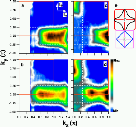
FIG. 1.: (color) Spectral weight of Nd$-$LSCO with different doping levels, x, integrated within different energy windows near the Fermi level. (a). x=0.10, 30meV; (b). x=0.10, 300meV; (c). x=0.15, 30meV; (d). x=0.15, 300meV. The boundary of the spectral weight can be approximated as $\mid$k_x$\mid$=$\pi$/4 and $\mid$k_y$\mid$=$\pi$/4 lines (dashed white lines). In the inset of Fig. 1(a) is the in$-$plane electrical field component. For comparison, the LDA calculated Fermi surface is included in (e) where the top part shows the Fermi surface at $k_{z}$=0 (black line) and the lower part the Fermi surface at $k_{z}=\pi/c$ (blue line)[18].

The data in Fig. 1 is difficult to reconcile with the band structure calculations where the LDA calculated Fermi surface runs more or less diagonally ([1,-1] direction) (see Fig. 1(e))[18]. We have done a matrix element simulation for this measurement geometry and found that the spectral weight near ($\pi$/2,$\pi$/2) nodal region is suppressed compared with the ($\pi$,0) and (0,$\pi$) antinodal regions. Nevertheless, it is still impossible to reproduce the observed spectral weight confinement with straight boundaries parallel to [1,0] or [0,1] direction, even by considering matrix element effects as well as the $k_{z}$ effect. On the other hand, a simple stripe picture seems to capture the main characteristics of the data in Fig. 1 if one considers the low energy signal as mainly being from metallic stripes[6, 19, 20, 21, 22]. The momentum distribution function n(k) (Fig. 1(b) and (d)) then suggests two sets of Fermi surfaces, defined by the $\mid$k_x$\mid$=$\pi$/4 and $\mid$k_y$\mid$=$\pi$/4 lines, which can be understood as a superposition of two one$-$dimensional (1D) Fermi surfaces originating from two perpendicularly orientated stripe domains. The $\pi$/4 boundary lines are related to the fact that the stripes are approximately quarter$-$filled in the charge stripes[2].

However, the above rigid stripe model also leaves many questions unanswered. A prominent one relates to the fast dispersion seen along (0,0) to ($\pi$,0) direction within the 200 meV of the Fermi level, which implies a charge motion perpendicular to vertical stripes[6]. The concomitant carrier motion along stripes and transverse to stripes points to the possible existence of a nodal state along the [1,1] diagonal direction which has zero superconducting gap in d$-$wave pairing symmetry. However, as seen from Fig. 1, as well as previous measurements for underdoped samples[23, 6], there is little spectral weight observed near the nodal region.

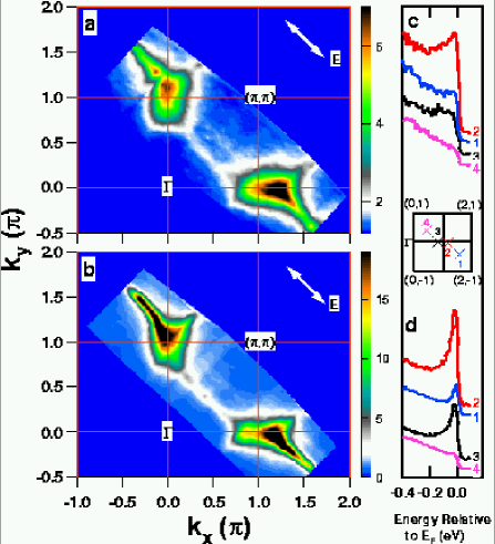
FIG. 2.: (color) Spectral weight of Nd$-$LSCO (x=0.15) (a) and LSCO (x=0.15) (b) integrated within 30 meV energy window near the Fermi level. Typical EDC spectra near the nodal and the ($\pi$, 0) regions, as indicated in the in$-$between inset, are shown in (c) and (d) for Nd$-$LSCO and LSCO, respectively. The in$-$plane electrical field is also indicated which was fixed during the measurement.

To gain more insight into the issue of nodal state, we focused our measurements on the nodal regions by covering along the diagonal direction (Fig. 2). We also extended the measurement to the second zone by considering possible different matrix element for different zones, as well as sharpening of spectral line in the second zone due to the negative dispersion velocity involved[24]. In order to enhance the signal from the nodal region, the in$-$plane electric field is maximized by fixing the $\overrightarrow{E}$ vector parallel to the sample surface; the measurement was fulfilled by rotating the analyzer, thus avoiding the complications of varying polarization. Our matrix element simulations show spectral weight enhancement in the nodal region for this measurement geometry. Fig. 2 shows the low energy excitations for both Nd$-$LSCO (x=0.15) and La_1.85Sr_0.15CuO₄ samples, measured under such a geometry. One sees the similar straight segments near (0,$\pi$) and ($\pi$,0) as seen in Fig. 1 even though the a-b plane of the samples were rotated 45 degrees with respect to each other. More importantly, it is possible to see the spectral weight near d$-$wave nodal region for both samples, although the signal in the first zone is weaker than that in the second zone. The EDC spectra near the nodal regions show a well$-$defined Fermi cut$-$off (Fig. 2(c) and (d)), indicating the metallic nature of these systems.

As seen from Fig. 1 and 2, there are two aspects involved in the electronic structure of the stripe phase. The first is the straight segment near the ($\pi$,0) and (0,$\pi$) antinodal regions. This feature is very robust as it is seen under different measurement geometries, which appears to be a measure of the ordered nature of stripes. The second feature is the nodal state seen in Fig. 2, which is sensitive to doping and measurement geometry. This feature is likely a measure of the deviation from ideal stripe case, which may be due to disorder or dynamic fluctuations. We note here that we have observed similar two features in Nd$-$LSCO with x=0.10 and in LSCO with doping level as low as x=0.07[25]. The nodal signal appears to get stronger with increasing Sr doping for both Nd$-$LSCO and LSCO, and for a given Sr doping level, it is stronger in Nd$-$free LSCO than in Nd$-$LSCO samples[25]. As seen from Fig. 2(a) and (b), near the ($\pi$,0) region in the second zone, the maximum intensity contour extends all the way from the nodal region and intersects with the ($\pi$,0)$-$(2$\pi$,0) line, suggesting an electron$-$like Fermi surface. Interestingly, this Fermi surface is reminiscent of that from the LDA calculation (Fig. 1(e))[18].

A complete description of the electronic structure of the stripe phase needs to take both of the above two aspects into account: the straight segment near the antinodal region and the spectral weight near the nodal region with its associated Fermi surface. Fig. 3 highlights these two features in the first Brillouin zone for the Nd$-$LSCO (x=0.15) and LSCO (x=0.15) samples, which are also schematically depicted in Fig. 3(c) (upper$-$left panel). While it seems to be straightforward to associate the straight segments with stripes because of their 1D nature[19], the detection of spectral weight near the nodal region in the static stripe phase poses a new challenge to our understanding of this charge ordered state because the nodal spectral weight is usually expected to be suppressed in a simple stripe picture[20, 21]. The experimental question regarding the origin is whether they originate from another distinct phase or they are intrinsic properties of the same stripe phase. In the case of phase separation, this would mean that, besides stripes, there is another non$-$stripe metallic phase with a much higher carrier concentration, as estimated from the Luttinger volume of the diamond$-$shaped Fermi surface (Fig. 3). As far as we know, there is little evidence of such a phase separation in Nd$-$LSCO and LSCO systems at the doping level discussed here[23], although it has been observed in a related La₂CuO_4+δ system[11].

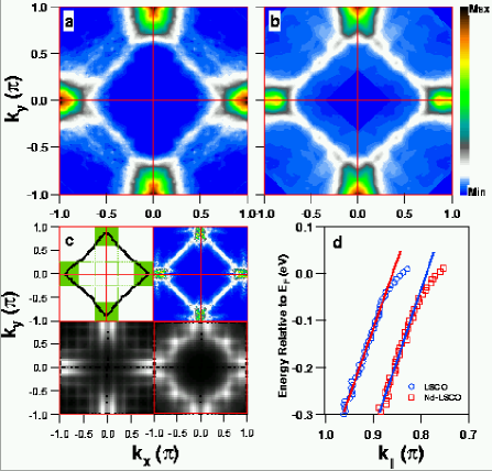
FIG. 3.: (color) Measured low energy (30meV integration) spectral weight of Nd$-$LSCO (x=0.15) (a) and LSCO (x=0.15)(b), as obtained by symmetrizing the first zone data of Fig. 2. The observed two features are schematically illustrated in (c) (upper$-$left panel): diamond$-$shaped nodal Fermi surface (black line) and 1D spectral confinements near ($\pi$,0) and (0,$\pi$) regions. The spectral weight patterns calculated from stripe fluctuation (upper-right panel)[19], from the site-centered stripe (lower$-$left panel) and bond$-$centered stripe (lower$-$right panel) [26] are also included in (c) for comparison. Fig. 3(d) shows the dispersion along the nodal direction (in the second zone) for the Nd$-$LSCO and LSCO samples; a slope breakdown in the dispersion can be seen for both cases at nearly -50meV. The dispersion for Nd$-$LSCO is horizontally offset for clarity, with the two solid lines as guide to the eye.

The detection of nodal spectral intensity in the stripe system provides a clear distinction of the stripe physics from the ordinary 1D charge motion in a rigid one$-$dimensional system. In the stripe context, the nodal Fermi surface may arise from disorder or fluctuation of stripes where the holes leak into the antiferromagnetic region[19, 22]. Here disorder also induces the effect that the antiferromagnetic region may not be fully gapped when it becomes very narrow. The measured spectral weight in Fig. 3 for Nd$-$LSCO and LSCO is similar to the one calculated based on such a disordered stripe picture (Fig. 3(c), upper$-$right panel)[19]. This also seems to be consistent with the trend that in LSCO the nodal spectral weight is more intense than that in Nd-LSCO because the stripes in the former are dynamic while they are static in the latter. Note that, in this picture, the nodal Fermi surface is actually a superposition of Fermi surface features from two perpendicular stripe domains; for an individual stripe domain, this Fermi surface feature can be discrete[19, 22].

An alternative scenario to understand the two features in the stripe context is a possible coexistence of site$-$ and bond$-$centered stripes[26]. Both types of stripes are compatible with neutron experiments[2], and are close in energy as indicated by various calculations[27]. As shown in Fig. 3(c), the calculated A(k,E_F) patterns for the site$-$centered (lower$-$left panel) and bond$-$centered stripes (lower$-$right panel)[26] bear a clear resemblance to the data in Fig. 1 and Fig. 2, respectively. It is therefore tempting to associate the 1D straight segment to site$-$centered stripes and the nodal Fermi surface feature to bond$-$centered stripes. Since these two types of stripes are different in their wave functions, it may also help explain why they show different behaviors under different measurement conditions. Moreover, the sudden slope change (or ”kink”) of the dispersion along the nodal direction for both Nd$-$LSCO and LSCO (Fig. 3(d)) is also consistent with this scenario[21, 26]. If this picture proves to be true, it would imply that, with increasing doping, bond$-$centered stripes are produced at the expense of site$-$centered stripes, and more bond$-$centered stripes may be generated as the stripes become more dynamic (Fig. 3). This seems to further suggest that the bond$-$centered stripes are more favorable for superconductivity than the site$-$centered stripes, a possibility remains to be investigated further. We note that the above scenarios can be closely related to each other. Stripe disorder or fluctuation may naturally give rise to hole$-$rich and hole$-$poor regions as in phase separation case, particularly with the possible existence of stripe dislocations in the system. In the case of stripe fluctuation, the randomness in the stripe separations may necessarily give rise to a mixture of site$-$centered and bond$-$centered stripes.

We thank J. Denlinger and J. Bozek for technical support, S. Kivelson, J. Tranquda, A. Balatsky, W. Hanke, M. Zacher and M. Salkola for helpful discussions. The experiment was performed at the Advanced Light Source of the Lawrence Berkeley National Laboratory, which is operated by the DOE’s Office of Basic Energy Science, Division of Material Science, with contract DE-AC03- 76SF00098. The division also provided support for the work at SSRL. The work at Stanford was supported by NSF grant through the Stanford MRSEC grant and NSF grant DMR-9705210.

REFERENCES

- [1] For a review, see V. J. Emery, S. A. Kivelson, and J. M. Tranquada, cond-mat/9907228; J. Zaanen, J. Phys. Chem. Solids 59, 1769(1998), and references therein.
- [2] J. M. Tranquada et al., Nature 375, 561 (1995); J. M. Tranquada et al., Phys. Rev. B 59, 14712 (1999).
- [3] M. v. Zimmermann et al., Europhys. Lett. 41, 629(1998).
- [4] A. W. Hunt et al., Phys. Rev. Lett. 82, 4300 (1999).
- [5] T. Noda, H. Eisaki and S. Uchida, Science 286 265(1999).
- [6] X. J. Zhou et al., Science 286, 268(1999).
- [7] S. W. Cheong et al., Phys. Rev. Lett. 67, 1791(1991).
- [8] T. E. Mason et al., Phys. Rev. Lett. 68 1414(1992).
- [9] A. Bianconi et al., Phys. Rev. Lett. 76, 3412 (1996).
- [10] K. Yamada et al., Phys. Rev. B 57, 6165(1998).
- [11] B. O. Wells et al., Science 277, 1067 (1997); Y. S. Lee et al., Phys. Rev. B 60, 3643-3654 (1999).
- [12] H. A. Mook et al., Nature 395, 580-582 (1998); Nature 401, 145-147 (1999).
- [13] V. J. Emery et al., Phys. Rev. B 56, 6120 (1997).
- [14] S. A. Kivelson et al., Nature 393, 550(1998).
- [15] Z.X. Shen and D. S. Dessau, Phys. Rep. 253, 1(1995).
- [16] A. Bansil and M. Lindroos, Phys. Rev. Lett. 83, 5154 (1999).
- [17] Th. Straub et al., Phys. Rev. B. 55, 13473 (1997).
- [18] J.-H. Xu et al., Physics Letters A 120, 489(1987); W. E. Pickett, Rev. Modern Phys. 61, 433 (1989).
- [19] M. I. Salkola, V. J. Emery and S. A. Kivelson, Phys. Rev. Lett. 77, 155(1996).
- [20] T. Tohyama et al., Phys. Rev. Lett. 82, 4910 (1999).
- [21] M. Fleck et al., Phys. Rev. Lett. 84, 4962 (2000).
- [22] R. S. Markiewicz, cond-mat/9911108.
- [23] A. Ino et al., J. Phys. Soc. Jpn. 68, 1496 (1999); cond-mat/9902048; cond-mat/0005370.
- [24] E. D. Hansen et al., Phys. Rev. Lett. 80, 1766 (1998).
- [25] T. Yoshida, X. J. Zhou et al., unpublished work.
- [26] M. G. Zacher et al., cond-mat/0005473.
- [27] S. R. White and D. J. Scalapino, Phys. Rev. Lett. 80, 1272(1998).