[

Fluctuations in finite critical and turbulent systems

Abstract

We show that hyperscaling and finite-size scaling imply that the probability distribution of the order parameter in finite size critical systems exhibit data collapse. We consider the examples of equilibrium critical systems, and a statistical model of ecology. We explain recent observations that the probability distribution of turbulent power fluctuations in closed flows is the same as that of the harmonic 2DXY model.

]

Critical systems with identical symmetries, dimension and exponents are defined to be members of the same universality class; but must they also share the same probability distribution for the fluctuating variables or order parameters? And if two systems do indeed exhibit the same probability distribution, are they necessarily in the same universality class, in the conventional meaning of the term?

Recently, light has been shed on these issues by studies of the probability distribution functions (PDFs) of fluctuating quantities in finite critical systems. Bramwell, Holdsworth and Pinton (BHP) [1] observed data collapse for the two-dimensional XY model (2DXY) in the spin-wave regime at low temperatures and in statistical models of nonequilibrium dynamics which exhibit self-organized criticality (SOC). Even more remarkably, they found that the power fluctuations in a closed turbulent flow exhibit exactly the same form of data collapse, with a scaling function that is indistinguishable from the aforementioned statistical critical models. Taken at face value, these observations lend support to the notion that finite Reynolds number ($Re$) turbulence is indeed a critical state, and that there is a kind of super-universality between systems with different dynamics and even dimensionality.

The purpose of this Letter is to show that finite-size systems that are in the critical regime should be expected to exhibit just this sort of data collapse. The system in question may be either an equilibrium system near its critical point, or a nonequilibrium system that attains a critical state through fine-tuning or other mechanism for achieving scale invariance. However, we are unaware of any reason a priori to expect that the probability distribution should be super-universal, and indeed we exhibit a counter example. Finally, we argue that the apparent agreement between magnetic systems and experiments on closed turbulent flows, while interesting and genuine, is not indicative of the intrinsic behavior of turbulence; we propose an explanation for the observations that appears to explain not only the data collapse but the Reynolds number dependence as well.

Probability Distribution Data Collapse:- Let us now review in more detail the findings of BHP. They examined the 2DXY model in the harmonic approximation for temperatures well below the Kosterlitz-Thouless transition $T_{KT}$. Although in an infinite system the magnetization $\vec{M}$ should be identically zero, for a finite system there are large fluctuations, and they measured the probability distribution function (PDF) for a range of system sizes and temperatures.

The scaled PDFs of the magnetization below $T_{KT}$ collapse onto each other for different system sizes and temperatures, provided one works in the harmonic approximation and the correlation length, $\xi$, is larger than the system size. The scaling necessary to achieve this data collapse is that the independent variable ($\eta\equiv|M|$) is replaced by $y\equiv\eta-\left<\eta\right>/\sigma$, where $\sigma$ is a measure of the width of the PDF, such as the width at half maximum. A similar data collapse was seen in a statistical model of ecology [2], where the scaled probability distribution of species abundance in a region was found to be independent of its area. Pinton et al. [3, 4] performed experiments on confined turbulent flows maintained at constant Reynolds number and looked at the PDF of power fluctuations. These too showed data collapse across different Reynolds numbers. Remarkably the PDFs for the turbulence data and the 2DXY model overlap within the precision of the data.

Subsequently a number of SOC systems, such as the Bak-Tang-Weisenfeld sand pile model [5], the Sneppen depinning model [6], the auto igniting forest fire model [7] and a model for granular media [8], have been studied and they too seem to show data collapse with a PDF very similar to that observed in the turbulence experiment [9]. The same holds true of the 2D Ising and 2D site percolation models as well. This seems to suggest that the scaling form is independent of system attributes such as symmetry (discrete or otherwise), state (equilibrium or otherwise) etc.

A similar phenomena was noted a long time ago by Nicolaides and Bruce [10], who were interested in the question of whether a universality class is defined by the values of the critical exponents, or whether the probability distributions were common to members of the same universality class. They found that the PDF of the two dimensional Ising, spin $1$, and $\phi^{4}$ models all had the same form in finite systems.

In fact, the issue of data collapse is linked with the existence of hyperscaling. Let us begin with a discussion of data collapse in equilibrium systems. In finite size magnetic systems, the PDF has a scaling form in the critical region [11], $P_{L}(M)=L^{\beta/\nu}\widetilde{f}({L/\xi},ML^{\beta/\nu})$, where $\widetilde{f}$ is a scaling function, $\beta$, $\nu$ are the critical exponents for the order parameter $M$ and the correlation length $\xi$ respectively, and $L$ denotes the linear dimension of the system, assumed to be in $d$ dimensions.

Near the critical point the correlation length becomes larger than the system size and making the unjustified assumption (a priori) that $\widetilde{f}$ is analytic in the first argument, we obtain $P_{L}(M)=L^{\beta/\nu}\widetilde{f}(ML^{\beta/\nu}).$ The sum rule for the static susceptibility $\chi_{T}$ implies that $k_{B}T\chi_{T}\sim L^{\alpha}[\left<M^{2}\right>-\left<M\right>^{2}]$. Notice that the quantity in the brackets is the variance of the probability distribution of the magnetization. The finite size scaling form for the susceptibility is $\chi_{T}=L^{\gamma/\nu}F({L/\xi})$ In the limit $\chi/L$ goes to infinity the scaling function $F$ tends towards a constant. Thus the measure of the width of the fluctuations, $\sigma$, scales as $\sigma^{2}\equiv\left<M^{2}\right>-\left<M\right>^{2}\sim L^{{\gamma/\nu}-d}$

BHP found that $\sigma P(M/\sigma)$ is a universal function, independent of system size. To test this, compute the function $\sigma P(M)=L^{{\gamma/2\nu}-d}L^{\beta/\nu}f(ML^{\beta/\nu})$,

$$\sigma P({M/\sigma})=L^{(\gamma+2\beta-d\nu)/2\nu}f({M/\sigma}L^{{\beta/\nu}+{\gamma/2\nu}-{d/2}})$$ (1)

Combining the hyperscaling relation, $2-\alpha=d\nu$ and Rushbrooke scaling, $\alpha+2\beta+\gamma=2$ gives $\gamma+2\beta=d\nu$. Given this identity it follows that all $L$ dependence in ($1$) disappears and we are left with a statement of data collapse:

$$\sigma P({M/\sigma})=f({M/\sigma})$$ (2)

Thus as long as finite-size scaling holds true near the critical point and hyperscaling is obeyed, the data, for different sizes, fall on top of each other for a given system. To our knowledge, this was first observed empirically by Nicolaides and Bruce [10].

There are interesting consequences for the moments of the PDF, $P$, illustrated here for the first two. The mean of the distribution is

$$\left<M\right>={\int MP(M)dM\over\int P(M)dM}\sim\sigma{\int zF(z)dz\over\int F(z)dz}$$ (3)

where $F$ is a scaling function

The integral is a pure number, so that the ratio of the mean and the variance is independent of $L$ ($\left<M\right>\sim\sigma$).

The moment relation is a direct result of hyperscaling, ${\left<M\right>}\sim{L^{\beta/\nu}},{\sigma}\sim{L^{{\gamma/2\nu}-{d/2}}}$

$${\left<M\right>\over\sigma}\sim{L^{-{2\beta+\gamma-d\nu/2\nu}}}$$ (4)

Hyperscaling then requires the $L$ dependence in the last line above to vanish. This relation between the mean and variance has been explicitly calculated for the $2$D XY in the spin wave approximation[9]. The moments of the order parameter satisfy, ${\mu_{n}}={g_{n}(g_{2}/2)^{-n/2}\sigma^{n}}$ and ${\mu_{n}}\sim{\mu_{1}^{n}\sim\sigma^{n}}$ implying

$$\sigma\sim{\mu_{1}\sim\left<M\right>}$$ (5)

Probability Distribution Data Collapse in an Ecology Model:- This scaling is fundamental to data collapse and holds even for systems not in thermal equilibrium. In particular it holds for the ecology model mentioned earlier. Harte et al. [2] proposed a model for the species abundance distribution observed in nature. It has been empirically observed that the number of species $S$ in a patch of area $A$ obeys a scaling law,$S\sim A^{z}$. Presumably this is an asymptotic in time form of a more general dynamical model, as the time evolution within this model is not specified. Nevertheless one can construct a recursion recursion relation for the PDF, $P_{i}(n)$, the probability for finding a species with $n$ individuals in a patch $i$. Patches $i$ are constructed by successive bifurcation of an initial biome. The key ingredient of the model is the assumption of self similarity, which forces the species-area law, but allows the probability distribution for the number of species resident in a biome to be calculated. If a species is found in area $A_{i}$, then there is a non-zero probability $a$, for finding it in one of the two halves (area $A_{i+1}=A_{i}/2$,) which is independent of $i$. The independence on scale $i$ of the probability $a$ gives rise (or more accurately, is equivalent) to the species-area rule, with $a=2^{-z}$. The resulting equation turns out to be

$$P_{i}(n)=xP_{i+1}(n)+(1-x)\sum_{k=1}^{n-1}P_{i+1}(n-k)P_{i+1}(k)$$ (6)

where $x=2(1-a)$. The variance of this PDF was computed by Banavar et al. [12]:

$$\sigma_{i}^{2}=\sum_{j=0}^{m-i-1}(2-x)^{j}(2-x)^{m-i-1}x(1-x)$$ (7)

where $m$ is defined as the maximum number of times the system can be subdivided before no species exist on the smallest patch ($P_{m}(1)=1$). When the system size is much bigger than the size of this smallest patch, the variance obeys a simple recursion relation, ${\sigma_{i}/\sigma_{i+1}}\sim 2-x$. The data collapse observed for this model is the statement ${\sigma_{i}P_{i}(n)}={\sigma_{i+1}P_{i+1}(n^{\prime})}$ and ${n/\sigma_{i}}={n^{\prime}/\sigma_{i+1}}$. It can be shown[13] that the PDF satisfies a finite-size scaling relation of the form $P_{i}(n)={1/n}f({n/N_{i}^{\phi}})$, where $\phi$ is a crossover scaling exponent, $N_{i}$ is the number of individuals of all species in biome patch $i$, and $N_{i+1}^{\phi}=2^{-\phi}N_{i}^{\phi}$; then the data collapse is equivalent to a relation between the exponents.

$${f({n\over N_{i}^{\phi}})}={f({n\over(2-x)N_{i}^{\phi}2^{-\phi}})}$$ (8)

leading to $2-x={2^{\phi}}$ which is equivalent to $\phi+z=1$.

This relation is nothing but the hyperscaling relation observed in the magnetic system. This can be seen by considering the asymptotic forms of the mean and variance of the PDF, ${<n>}\sim{N^{\phi}}$ and ${\sigma}\sim{(2-x)^{m}\sim 2^{m\phi}}\sim{N^{\phi}}$. This immediately gives us the moment scaling which was crucial to data collapse and hyperscaling, $\sigma\sim\left<n\right>$. It is remarkable that the ecology model shows this behaviour for its moments – an unforseen consequence of the assumption of self-similarity.

Power fluctuations in a turbulent flow:- Having established the connection between hyperscaling (moment relationships) and data collapse let us turn our attention to the case of confined turbulent flows. The experiment consists of a closed cylinder in which a turbulent fluid is driven at the top and bottom by counter-rotating plates with vanes, moving at the same mean angular frequency. The PDFs for power fluctuations $\Pi$ were measured [3, 4] for different Reynolds numbers ($Re$) and found to exhibit data collapse. However the ratio of the mean to the variance depended on $Re$: $\Pi_{rms}/\overline{\Pi}\sim Re^{-\alpha},\hskip 14.22636pt\alpha\sim 0.33$.

This observation shows that the Reynolds number, and hence the extent of the inertial range, is not the parameter that controls the nature of the fluctuations: it is not analogous to the finite size of the system, as has been suggested previously. If this suggestion were correct, hyperscaling would have required that the ratio of mean to variance be independent of Reynolds number.

Our analysis suggests that the relevant parameter, in the case of the confined flows, that controls the nature of the fluctuations is not the Reynolds number but the physical system size itself. In addition to the scaling analysis mentioned above, the reasons for this is two fold. First, the experiments were performed by changing either the fluid (i.e. viscosity) or the angular velocity (see Ref. 3 and 4 for details of the experiment) and not by changing the spatial dimensions of the flow. Second, it was also noted that an open flow did not exhibit any non-Gaussian fluctuations in the total power dissipated. In other words the fluctuations are not governed by the degrees of the turbulent flow (i.e. Reynolds number) but the degrees of freedom of coherent structures that form in these system which in turn depends on the system size, $L$.

We hypothesize that the flow is composed of a turbulent region around the top plate with a mean angular momentum, another oppositely directed turbulent region around the bottom plate, and an interfacial region between them – a shear pancake. Experiments were performed in both open and closed geometries, which differ by the absence or presence of a confining cylindrical wall. In the open geometry, the power fluctuations of each plate were non-Gaussian, and negatively skewed, while the total power (sum of the power measured at each plate) fluctuations were Gaussian. In the closed geometry all of these three quantities were non-Gaussian, with a scaled probability distribution apparently indistinguishable from that of the 2D XY model simulations.

In the open geometry, the shear pancake can shift its mean vertical position instantaneously as shear energy is dissipated horizontally, but in the closed geometry, this is not possible because of the walls. In the open geometry, as the shear pancake moves, the net turbulent energy in the upper half of the cell will increase/decrease while that in the lower half of the cell will decrease/increase: hence, we anticipate that the power fluctuations should be anti-correlated, in agreement with observations[14].

In the closed geometry, we can describe the shear pancake by its height $h(x,y)$ above the $x$, $y$ plane positioned parallel to and equidistant from the rotating plates. The shear pancake experiences random fluctuations from the turbulent flows, which drive it with an effective, Reynolds number dependent temperature $T(Re)$ and Boltzmann distribution $P_{h}(h)\propto\exp[-S(h)/T]$. The action $S(h)$ describes local height fluctuations of the shear pancake, and the power dissipation of the system should be expected to depend in some way on the friction between the two counter-rotating turbulent flows i.e. on the surface area of the shear pancake, and not its absolute mean height. Any local fluctuation increases the total surface area of the shear pancake and hence increases the power dissipation in both flows. Hence, in this case, we anticipate that the power fluctuations would be correlated, in agreement with observations[15]. Thus the action should be of the form

$$S(h)\propto\int dx\,dy\,\sqrt{1+(\nabla h)^{2}}\approx\int dx\,dy\,(\nabla h)^{2}$$ (9)

which is the Hamiltonian of the 2D XY model in the spin wave approximation, making the identification of $h$ with the phase $\theta$.

In order to complete the dictionary between the PDFs of the 2D XY model magnetization and the turbulent power, we note that the power dissipated is by hypothesis proportional to $S\{h\}$ and thus is linearly dependent on $(\nabla h)^{2}$. Similarly, the absolute value of the magnetization per spin $M$, measured in the 2DXY simulations (for $N$ spins $\vec{S}_{i}$) is given by $M\equiv\sqrt{\left(\sum_{i=1}^{N}\vec{S}_{i}\right)\cdot\left(\sum_{j=1}^{N}\vec{S}_{j}\right)}/N\approx 1-\frac{1}{4N}\sum_{ij}(\theta_{i}-\theta_{j})^{2},$ showing that the probability distribution of magnetization fluctuations is indeed the counterpart of the power fluctuations in the turbulent flow. It follows from our assumptions above that the probability distributions should be identical. Note that we are definitely predicting that the power probability distribution should be that of the 2DXY model in the harmonic approximation only. Indeed, we have simulated the 2DXY model for temperatures near the Kosterlitz-Thouless transition, and find significant deviations from the probability distribution for the turbulent power and the 2DXY model in the harmonic approximation as shown in figure 1 (and has also been noticed by Palme et al. [16]).

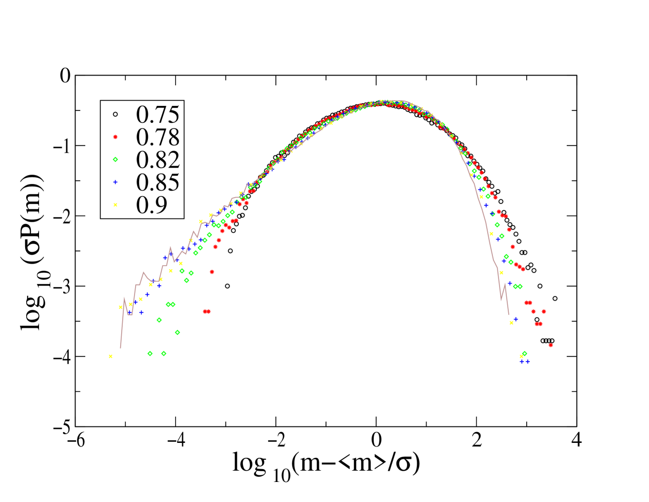
FIG. 1.: Probability distribution function of the magnetization in a 2DXY model for different values of temperature: $J/K_{B}T=0.75(\circ),0.78(*),0.82(\diamond),0.85(+)$ and $0.9(\times)$. The solid line represents the universal distribution of BHP [1].

Now, we discuss the Reynolds number dependence of the ratio $\mu/\sigma$. By hypothesis, this should be given by using the temperature dependence of $\mu/\sigma$ from the harmonic 2D XY model, but with $T$ given by $T(Re)$. To see how the effective temperature should scale with $Re$, note that the velocity of the flow scales as $R\Omega$ where $R$ is the radius of the plates, and $\Omega$ is the angular velocity. The net mass per unit height of the cylinder scales as $R^{2}$. Hence the net kinetic energy scales as $R^{4}\Omega^{2}$. The $Re$ number is proportional to $R^{2}\Omega$ so that the energy scales as $Re^{2}$. The number of degrees of freedom giving rise to this turbulent energy is proportional to $Re^{9/4}$, so that $T(Re)\sim Re^{-1/4}$. Using the fact that $\mu/\sigma\sim T$ [17] we obtain that $\mu/\sigma\sim Re^{-1/4}$, which agrees reasonably with the data, although the exponent is not the optimal fit to all the data points, as shown in figure 2.

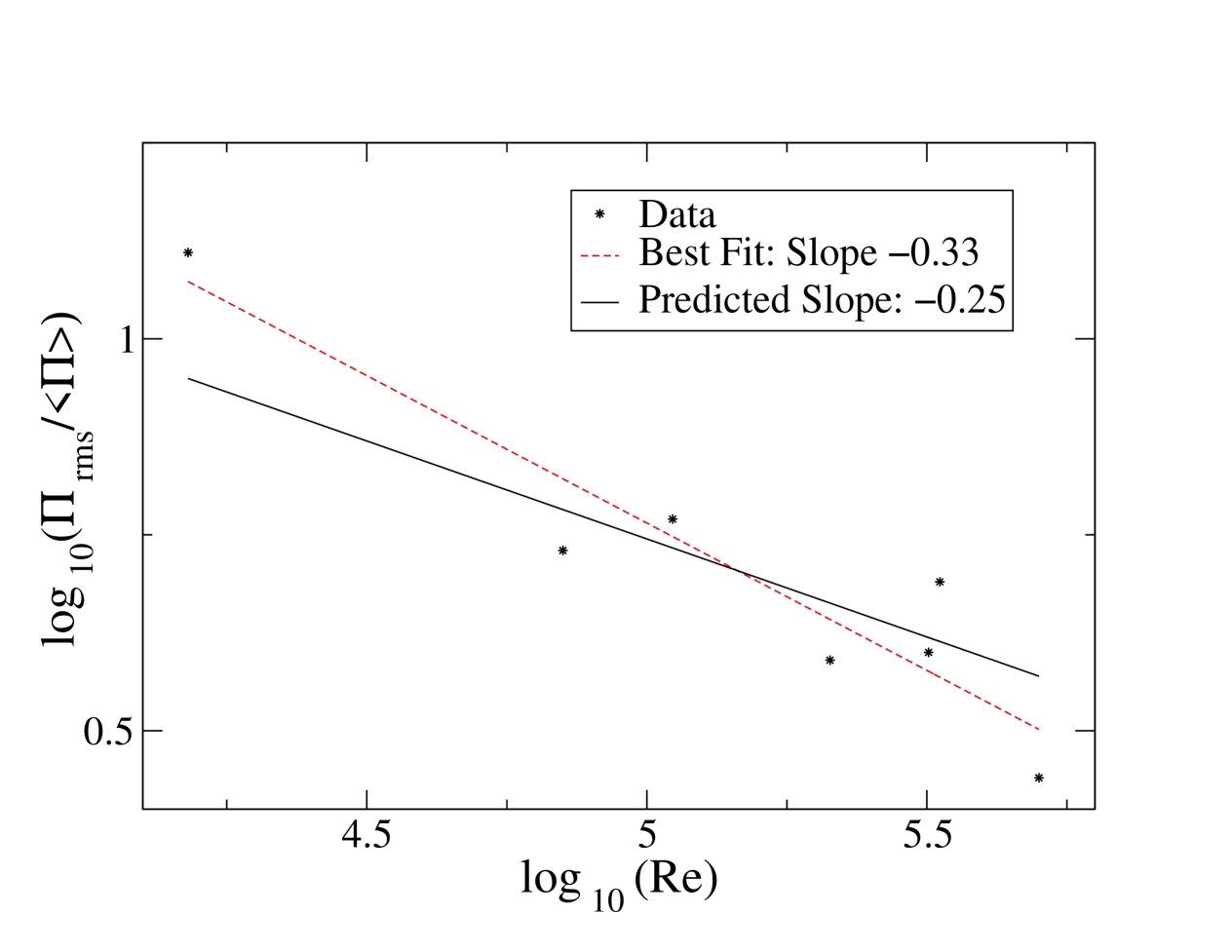
FIG. 2.: Data from J-F Pinton et al. [4] with the best fit and a fit to our predicted slope of -$0.25$.

Finally, we mention that the dynamic universality class of the height fluctuations should be the 2D Edwards-Wilkinson model [18]; implications of this for the time dependent correlations of the power will be discussed elsewhere.

In conclusion, we have shown how universal scaling phenomena can arise in finite critical systems due to hyperscaling; the observed similarity of the probability distribution scaling function in the harmonic 2DXY and a closed turbulent cell is a special case, and is not generic.

- [1] S.T. Bramwell, P.C.W. Holdsworth and J.-F. Pinton, Nature 396, 552 (1999).
- [2] J. Harte, A. Kinzig and J.L. Green, Science 284, 334 (1999).
- [3] R. Labbe, J.-F. Pinton and S. Fauve, J. Phys. II France 6, 1099 (1996).
- [4] J.-F. Pinton and P.C.W. Holdsworth, Phys. Rev E 60, R2452 (1998).
- [5] P. Bak, C. Tang and K. Weisenfeld, Phys. Rev. Lett. 59, 381 (1997).
- [6] K. Sneppen, Phys. Rev. Lett. 69, 3538 (1992).
- [7] P. Sinha-Ray, L.B. de Agua and H.J. Jensen, to be published.
- [8] E. Caglioti, V. Loreto, H. Hermann and M. Nicodemi, Phys. Rev. Lett. 79, 1575 (1997).
- [9] S.T. Bramwell et al., Phys. Rev. Lett 84, 3744 (2000). For other examples of order parameter fluctuations in finite systems see R. Botet and M. Ploszajczak, unpublished.
- [10] D. Nicolaides and A.D. Bruce, J. Phys. A:Math. Gen. 21, 233 (1988).
- [11] K. Binder, Computational Methods in Field Theory, edited by H. Gauslever and C.B. Lamb (Springer, Berlin, 1992).
- [12] J.R. Banavar, J.L. Green, J. Harte and A. Martin, Phys. Rev. Lett. 83, 4214 (1999).
- [13] H.G. Martin and Nigel Goldenfeld, unpublished.
- [14] See the ref. [4], figure 2(b).
- [15] See the ref. [4], figure 4(b).
- [16] G. Palma, T. Meyer and R. Labbe, unpublished.
- [17] P. Archambault, S.T. Bramwell and P.C.W. Holdsworth, J.Phys. A Math. Gen. 30, 8363 (1997).
- [18] S.F. Edwards and D.R. Wilkinson, Proc. Roy. Soc. A 38, 17 (1982).