Quantum tetrahedral mean field theory of the magnetic susceptibility for the pyrochlore lattice

Abstract

A quantum mean field theory of the pyrochlore lattice is presented. The starting point is not the individual magnetic ions, as in the usual Curie–Weiss mean field theory, but a set of interacting corner sharing tetrahedra. We check the consistency of the model against magnetic susceptibility data, and find a good agreement between the theoretical predictions and the experimental data. Implications of the model and future extensions are also discussed.

Introduction.- Geometrically frustrated antiferromagnets with a pyrochlore lattice exhibit a rich phenomenology which has received a vast amount of attention during the last decade hfm.2000 ; ramirez.1994 . In the pyrochlore lattice, the magnetic ions occupy the corners of a 3D arrangement of corner sharing tetrahedra. Materials that crystallize in this structure exhibit anomalous magnetic properties raju.1998 ; raju.1999 ; huber.2000 : The magnetic susceptibility follows the Curie–Weiss law down to temperatures well below the Curie temperature. Some of them exhibit long range order at very low temperatures, whereas others behave as spin glasses, even though the lattice is almost perfect. There are other compounds of this class that show short range order, and are regarded as spin liquids.

In spite of the intensive research in these systems during the last decade, there is still a lack of critical comparison between theory and experiment. Even though there are a number of models and classical Monte Carlo simulations moessner.1999 which qualitatively describe some of the experimental results, some of the features found in the experimental data cannot be explained by means of a classical theory, as are, for example, the maxima appearing in the magnetic susceptibility at very low temperatures, which a classical model cannot explain. However, there have been few attempts to investigate these systems quantum mechanically. Harris and co–workers have studied the quantum $s=\frac{1}{2}$ Heisenberg antiferromagnet harris.1991 . Canals and Lacroix canals.1998 , have applied a perturbative approach to the density operator of a small cluster, and found that the ground state is a quantum spin liquid.

In this work, we undergo the task of making such a quantum theory of the pyrochlore lattice in the framework of the mean field theory. The goal of this work is twofold: In one hand, we introduce a fully quantum mechanical mean field theory of the Heisenberg antiferromagnet in the pyrochlore lattice for arbitrary spin $s$. In the other hand, we try to make this model as simple as possible, in order to make it easy to compare it with experimental data and extract information about the various interactions that play a role in these systems. Only the main results of the model will be presented here, as a more detailed presentation of the model will be published elsewhere. The starting point to build this MF is not a set of interacting spins, but a set of coupled tetrahedra, which goes back to the constant coupling approximation of Kastelejein and van Kranendonk kastel.1956 . The magnetic susceptibility of this system is calculated for both the interacting and non–interacting tetrahedra cases. We find that the independent tetrahedra model fails to explain the behavior of experimental data, and we justify this fact, whereas the MF theory describes quasi–quantitatively the experimental data for a variety of systems.

The model.- The Hamiltonian of the quantum Heisenberg model with nearest neighbors in the presence of an applied magnetic field $H_{0}$ in the pyrochlore lattice can be put as smart.1966

$$H=-2J_{1}\sum_{\left\langle i,j\right\rangle}\vec{s}_{i}\cdot\vec{s}_{j}-H_{0}\sum_{i}s_{z_{i}},$$ (1)

where $J_{1}$ is the negative exchange coupling, and $\vec{s}_{i}$ is the spin operator of the $i$–th magnetic ion. The Zeeman term has been quoted in units of the Bohr magneton times the gyromagnetic ratio, so $H_{0}$ has dimensions of energy.

We start by considering the magnetic susceptibility of one tetrahedron. In this simple case, the Hamiltonian can be easily diagonalized in terms of the total spin representation of the tetrahedron, and the magnetization can be expressed as

$$M=\frac{\sum_{S}g(S)Se^{j_{1}S(S+1)}Q_{S}(x)}{\sum_{S}g(S)e^{j_{1}S(S+1)}\frac{\sinh\left(\frac{2S+1}{2S}x\right)}{\sinh\left(\frac{x}{2S}\right)}},$$ (2)

where $S$ represents the modulus of the total spin operator of the tetrahedron; $g(S)$ is the degeneracy associated to the total spin value $S$, which can be calculated by using Van Vleck’s formula vanvleck.1959 , and are listed in table 1 for the values of the individual spins $s$ considered in this work;

	$S$
	0	1	2	3	4	5	6	7	8	9	10	11	12	13	14
$s=1$	3	6	6	3	1
$s=\frac{3}{2}$	4	9	11	10	6	3	1
$s=\frac{5}{2}$	6	15	21	24	21	15	10	6	3	1
$s=\frac{7}{2}$	8	21	31	38	42	43	41	36	28	21	15	10	6	3	1

Table 1: Values of $g(S)$ for the individual spins, $s$, considered in this work.

$x=\frac{H_{0}S}{T}$, and $j_{1}=\frac{J_{1}}{T}$ (the energies are quoted in units of the Boltzmann constant, so they have dimension of absolute temperature); and

$$Q_{S}(x)=\frac{2S+1}{2S}\frac{\cosh\left(\frac{2S+1}{2S}x\right)}{\sinh\left(\frac{x}{2S}\right)}-\frac{1}{2S}\frac{\sinh\left(\frac{2S+1}{2S}x\right)}{\sinh\left(\frac{x}{2S}\right)}\coth\left(\frac{x}{2S}\right).$$ (3)

In the limit $x\ll 1$, we can define the magnetic susceptibility of the tetrahedron as

$$\chi^{tet}=\frac{M}{H_{0}}=\frac{1}{T}\frac{\sum_{S}g(S)S(S+1)(2S+1)e^{j_{1}S(S+1)}}{\sum_{S}g(S)(2S+1)e^{j_{1}S(S+1)}}.$$ (4)

The susceptibility per ion in the tetrahedron will be simply given by $\hat{\chi}^{tet}=\frac{\chi^{tet}}{4}$.

It is interesting to note that for $j_{1}\ll 1$, the susceptibility can be identified with the high temperature expansion of a Curie–Weiss type law (per ion and in the same units we are considering in this work), $\hat{\chi}^{tet}=\frac{s(s+1)}{3T}\left(1+\frac{\theta}{T}\right)$, where $\theta=2s(s+1)J_{1}$. Therefore, this model reproduces the behavior predicted by the Curie law at very high temperatures. However, the value of the Curie–Weiss temperature in this type of lattice is given by smart.1966

$$\theta^{CW}=4J_{1}s(s+1)=2\theta.$$ (5)

The reason for this deviation is, obviously, the fact that we have not considered the interaction with the neighboring tetrahedra, which is of the same order of magnitude that the interactions inside the tetrahedron.

To remedy this situation, we can introduce a tetrahedral mean field (TMF) theory that takes into account, at least in an approximate way, the interaction with the neighboring ions outside the tetrahedron. Each ion in the tetrahedron interacts with $z=3$ external ions, in the nearest neighbor interaction approximation.

The effect of this interaction with the nearest neighbors outside the tetrahedron, in the spirit of the MF theory, can be accounted for by introducing a molecular field proportional to $z$ and the magnetization per ion $m=\frac{M}{4}$. The constant of proportionality can be put without loss of generality as $2J_{eff}$. In the high temperature limit, the magnetization per ion can be put as $m=\hat{\chi}^{tet}\,\left(H_{0}+2zJ_{eff}m\right)$, from which we obtain the expression of the susceptibility in this tetrahedral mean field (TMF) model

$$\chi^{tmf}=\frac{\hat{\chi}^{tet}}{1-2z\,J_{eff}\,\hat{\chi}^{tet}}.$$ (6)

The value of the $J_{eff}$ parameter can be estimated as follows: in the high temperature limit, $\chi^{tmf}$ can be put again as the high temperature expansion of a Curie–Weiss type law. By equating this expansion with the real Curie–Weiss law up to $\frac{1}{T^{2}}$ terms, we reach at the condition

$$\theta+2z\,J_{eff}\frac{s(s+1)}{3}=\theta^{CW}.$$ (7)

Were the interaction with further neighbors negligible with respect to the first neighbor interactions, relation (5) would be exact and, therefore, by using the relation between $\theta$ and $J_{1}$ obtained in the non–interacting tetrahedra case, we would have $J_{eff}=J_{1}$, which is completely similar to the value obtained in the standard mean field theory.

Of course, second and further nearest neighbor interactions are always present in real systems. Thus, the value of $\theta^{CW}$ obtained from experimental data can contain additional contributions coming from next nearest neighbors and so on. For this reason, relation (5) is only an approximate one, and so is (7). In order to compare the predictions of the model with experimental measurements, it is preferable to consider the interaction inside the tetrahedron, $J_{1}$, and the interaction with nearest neighbors outside the tetrahedron, $J_{eff}$, as adjustable parameters. The difference between $J_{1}$ and $J_{eff}$ provides a way of estimating the value of additional interactions not explicitly accounted for in this model. In fact, interactions with further neighbors can be explicitly accounted for in this model in the following way: let us consider the interaction with $z^{\prime}$ next nearest neighbors (9 for the pyrochlore lattice) in the mean field approximation. In this case, the magnetization per ion will be given by $m=\hat{\chi}^{tet}\,\left(H_{0}+2zJ_{1}m+2z^{\prime}\,J_{2}m\right)$, where $J_{2}$ represents the coupling with next nearest neighbors, and the magnetic susceptibility is given by

$$\chi^{tmf}=\frac{\hat{\chi}^{tet}(J_{1},T)}{1-6(J_{1}+3J_{2})\,\hat{\chi}^{tet}(J_{1},T)},$$ (8)

where we have made use of the fact that for the pyrochlore lattice $z=3$ and $z^{\prime}=9$ and that the difference between $J_{1}$ and $J_{eff}$ comes from these additional interactions, that is, $J_{eff}=J_{1}+3J_{2}$.

Comparison with experimental data.- In order to test the validity of the above model, it is important to compare its predictions with magnetic susceptibility data. We have selected the following systems whose magnetic ions form a pyrochlore lattice: ZnCr₂O₄ huber.2000 , Gd₂Ti₂O₇ raju.1999 , Y₂Mo₂O₇ greedan.1986 , and CdFe₂O₄ Ostorero.1989 , where the value of the magnetic ion spin is $s=\frac{3}{2}$, $s=\frac{7}{2}$, $s=1$, and $s=\frac{5}{2}$, respectively.

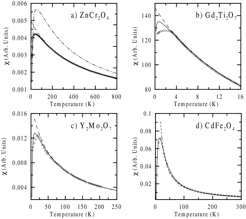
Figure 1: Comparison with experimental susceptibility data of (a) ZnCr₂O₄, (b) Gd₂Ti₂O₇, (c) Y₂Mo₂O₇, and (d) CdFe₂O₄. The open circles represent experimental data, whereas the solid lines are fits to expression (8). The dashed lines represent fits to the Curie–Weiss law. The dot–dashed line in the case of ZnCr₂O₄ represents the prediction of the isolated tetrahedra model with the parameters obtained from the fit to the Curie–Weiss law.

The temperature dependence of the magnetic susceptibility in these materials can be seen in fig. 1. All of them follow a Curie–Weiss law from high temperatures to well below the Curie–Weiss temperature. The predictions of our TMF theory are also plotted in fig. 1. The values of $J_{1}$ and $J_{2}$, which we obtain by fitting the data points above $T_{c}$, have been quoted in table 2. Here $T_{c}$ marks the transition to the low temperature phase, which is either long range order (LRO) or spin–glass (SG). The data for Gd₂Ti₂O₇ are from AC susceptibility measurements. Also, the predictions of the non–interacting tetrahedra model have been represented for the case of ZnCr₂O₄, in order to show the deviations of the predictions of this model from the experimental data. The case of CdFe₂O₄ is somewhat special and will be analyzed below.

As we can see from observation of the figure and the values collected in table 2, the agreement between theory and experiment is quite good. In the case of ZnCr₂O₄, the agreement is excellent in the entire temperature range. For the other two systems, there is only qualitative agreement. Nevertheless, we feel that the agreement between theory and experiment is good enough to assess the validity of our model, at least, from a qualitative point of view.

It is important to notice that the values predicted for $J_{1}$ are systematically smaller than the values of $J_{eff}=J_{1}+3J_{2}$, which are close to the ones obtained from fits to a Curie–Weiss law, which is consistent with the idea mentioned in the previous section about additional interactions from further neighbors.

Material	$\theta^{CW}$	$J^{CW}$	$T_{m}^{exp}$	$T_{c}$	$J_{1}$	$J_{2}$	$T_{m}^{fit}$
ZnCr2O4	-388	-25.9	37.4	12 (LRO)	-19.2	-2.3	38.0
Gd2Ti2O7	-21	-0.33	2.0	0.97 (LRO)	-0.20	-0.05	0.7
Y2Mo2O7	-61	-7.625	–	18 (SG)	-7.13	-0.02	11.2
CdFe2O4	0	0	17.0	10 (LRO)	-5.23	4.1	14.4

Table 2: Parameters of the TMF theory. All of them are quoted in K.

An additional prediction of our model is the existence of a maximum appearing in the $\chi$ versus $T$ plots. The position of this maximum, $T_{m}$, presented in table 2, can only be calculated numerically, as its determination involves solving a transcendental equation. However, it is found that it follows this empirical law

$$T_{m}=-\frac{(s+1)\,J_{1}}{1.273}.$$ (9)

It is important to notice that the position of the maximum is determined only by the value of the interaction inside the tetrahedron. We see that the value of $T_{m}$ predicted by the model in the case of ZnCr₂O₄ is very close to the experimental value. However, in the case of Gd₂Ti₂O₇ the predicted maximum occurs at $\sim 1/2$ of the experimental value. In the case of Y₂Mo₂O₇ there is no maximum in the paramagnetic phase as there is a transition to a SG at around 18 K.

As commented above, the case of CdFe₂O₄ is especial, because in this material, next nearest neighbor interactions are of the same order of magnitude than the nearest neighbor ones, but ferromagnetic, which leads to an experimental value of the Curie–Weiss temperature equal to zero. However, the present model is able to describe even this limiting case, and the values of the various couplings obtained from the fit are very reasonable. Moreover, the position of the maximum predicted by the model is in very good agreement with the experimental value, and inside the experimental uncertainty.

Conclusions.- In this work we have analyzed the temperature dependence of the magnetic susceptibility data of an arrangement of magnetic ions of spin $s$ in a pyrochlore lattice. To do this, we have developed a tetrahedral mean field theory taking as a starting point the exact susceptibility of a set of four interacting spins in the corners of an isolated tetrahedron. For the sake of completeness, we have also briefly analyzed the susceptibility predicted by a non–interacting tetrahedra model. We reach the conclusion that, even though the non–interacting model provides an adequate description of the high temperature region, it fails to quantitatively describe the temperature dependence of the susceptibility at lower temperatures, as the $\frac{1}{T^{2}}$ term in this model is $\frac{1}{2}$ of the actual value. However, once we incorporate the interactions with the rest of nearest neighbors in terms of a mean field, we find a quite good agreement between the theoretical predictions and experimental data. Especially important is the prediction of the appearance of a maximum in $\chi$ versus $T$. The position of the maximum has been calculated, and a reasonable agreement is found. At this point, it is very difficult to say if the deviations are an intrinsic problem of the model. To clarify this point, more good quality experimental data in a variety of systems whose susceptibility maxima lie well above $T_{c}$ would be necessary.

One feature of this model is that it can be very easily generalized to include additional interactions coming from further neighbors and more exotic systems where, for example, the interaction with the nearest neighbors is antiferromagnetic and is ferromagnetic with next nearest neighbors, as we have done for the case of CdFe₂O₄, finding a very good agreement between theory and experiment.

Of course, this work is not conclusive, in the sense that it does not solve the problem of the anomalous behaviors found in these types of systems. It does not provide an explanation of why some of these materials exhibit a long range order state at very low temperatures, whereas other are in a spin liquid state. Moreover, nothing has been said about the disorder always present in any material, which has been suggested to be related to the appearance of behaviors characteristic of spin glasses. These subjects are out of the scope of this paper, though they should constitute the direction of future work.

In any case, we think that the present model provides a good starting point for such investigations.

- (1) Proceedings of the Highly Frustrated Magnetism 2000 conference (to be published in the Can. J. of Phys.)
- (2) A. P. Ramirez, Ann. Rev. Mater. Sci. 24, 453 (1994); P. Schiffer and A. P. Ramirez, Comments Condens. Mater. Phys. 18, 21 (1996).
- (3) N. P. Raju, J. E. Greedan, M. A. Subramanian, C. P. Adams, and T. E. Mason, Phys. Rev. B 58, 5550 (1998); Y. M. Jana and D. Ghosh, Phys. Rev. B 61, 9657 (2000); M. J. P. Gingras, C. V. Stager, N. P. Raju, B. D. Gaulin, and J. E. Greedan, Phys. Rev. Lett. 78, 947 (1997); J. S. Gardner, S. R. Dunsiger, B. D. Gaulin, M. J. P. Gingras, J. E. Greedan, R. F. Kiefl, M. D. Lumsden, W. A. MacFarlane, N. P. Raju, J. E. Sonier, I. Swainson, and Z. Tun, Phys. Rev. Lett. 82, 1012 (1999); J. E. Greedan, N. P. Raju, A. Maignan, Ch. Simon, J. S. Pedersen, A. M. Niraimathi, E. Gmelin, and M. A. Subramanian, Phys. Rev. B 54, 7189 (1996); S. T. Bramwell, M. N. Field, M. J. Harris, and I. P. Parkin, J. Phys.: Condens. Matter 12, 483(2000).
- (4) N. P. Raju, M. Dion, M. J. P. Gingras, T. E. Mason, and J. E. Greedan, Phys. Rev. B 59, 14489 (1999).
- (5) N. O. Moreno, H. Martinho, C. Rettori, A. J. García-Adeva, D. L. Huber, M. T. Causa, M. Tovar, W. Ratcliffe, S-W Cheong, and S. B. Oseroff (presented in the HFM2000).
- (6) R. Moessner and A. J. Berlinsky, Phys. Rev. Lett. 83, 3293 (1999); R. Moessner and J. T. Chalker, Phys. Rev. Lett. 80, 2929 (1998); R. Moessner, Phys. Rev. B 57, R5587 (1998); R. Moessner and J. T. Chalker, Phys. Rev. B 58, 12049 (1998); J. N. Reimers, A. J. Berlinsky, and A. C. Shi, Phys. Rev. B 43, 865 (1991).
- (7) A. B. Harris, A. J. Berlinsky, and C. Bruder, J. Appl. Phys. 69, 5200 (1991).
- (8) B. Canals and C. Lacroix, Phys. Rev. Lett. 80, 2933 (1998); Phys. Rev. B 61, 1149 (2000).
- (9) T. Oguchi, Prog. Theoret. Phys. (Kyoto) 13, 148 (1955); P. W. Kastelejein and J. van Kranendonk, Physica 22, 317 (1956).
- (10) J. S. Smart, “Effective field theories of magnetism” (Saunders, Philadelphia, 1966).
- (11) J. H. van Vleck, “The theory of electric and magnetic susceptibilities”, p. 323-324 (Oxford, London, 1959).
- (12) J. E. Greedan, M. Sato, Xu Yan, F. S. Razavi, Solid State Commun. 59, 895 (1986).
- (13) J. Ostoréro, A. Mauger, M. Guillot, A. Derory, M. Escorne, and A. Marchand, Phys. Rev. B 40, 391 (1989).