Path-integral formulation of stochastic processes for exclusive particle systems

Abstract

We present a systematic formalism to derive a path-integral formulation for hard-core particle systems far from equilibrium. Writing the master equation for a stochastic process of the system in terms of the annihilation and creation operators with mixed commutation relations, we find the Kramers-Moyal coefficients for the corresponding Fokker-Planck equation (FPE), and the stochastic differential equation (SDE) is derived by connecting these coefficients in the FPE to those in the SDE. Finally, the SDE is mapped onto a field theory using the path integral, giving the field-theoretic action, which may be analyzed by the renormalization group method. We apply this formalism to a two-species reaction-diffusion system with drift, finding a universal decay expoent for the long-time behavior of the average concentration of particles in arbitrary dimension.

In recent years, nonequilibrium phenomena such as nonequilibrium phase transitions, bifurcations, and synergetics have attracted much attention[2], not only because of their connections to a variety of important physical problems (pattern formation, morphogenesis, self-organization, etc.), but also because of the analytic challenge due to lack of a general formalism for nonequilibrium systems, in contrast to equilibrium statistical mechanics, which has well-established concepts and tools. In pursuit of a general formalism, statistical physicists have investigated nonequilibrium phase transitions in lattice models over the last decade[3]. As lattice models have played a central role in equilibrium statistical mechanics, they will also be important in nonequilibrium statistical mechanics. In particular, theoretical analysis of reaction-diffusion systems where both diffusion and reaction take place on the lattice is relevant to the understanding of a wide class of nonequilibrium phenomena in nature[4]. It has long been recognized that the mean-field rate equations are not applicable to reaction-diffusion systems in low dimensions. After Doi and others introduced the field-theoretic method using the bosonic coherent state path integral[5], Lee and Cardy using the renormalization group (RG) approach have improved on this method[6, 7] in the description of the anomalous kinetics in these systems. Assuming the systems are in the low density regime, Lee and Cardy rewrite the master equation for the Markov process as the bosonic Hamiltonian . The Hamiltonian in turn can be mapped onto field theory and analyzed by the renormalization group method in arbitrary dimensions. For simple models such as $A+A\rightarrow\emptyset$ and $A+B\rightarrow\emptyset$, this bosonic field-thoeretic method provided the correct time dependence for the density decay in low dimensions[6, 7, 8, 9].

Despite the successes achieved by the bosonic field theory for reaction-diffusion systems, there are still many open problems. Driven reaction-diffusion systems[10, 11], multi-species adsorption models[12], and epidemic models are some examples to which the bosonic field theory cannot be applied since the steady states of these systems cannot be assumed to be in a low density regime. In these systems, the hard-core property of the particles is important and the bosonic approach fails. In response to these challenges, there have been many attempts to take the hard-core property into account. Brunel et al.[13] and Bares and Mobilia[14] formulated fermionic field theories for a single-species reaction-diffusion process confined to one space dimension. However, these fermionic field theories are very hard to extend in practice to higher spatial dimensions or to multispecies processes.

We have focused on the extensibility of the field theory to multispecies processes and to higher spatial dimensions including the hard-core exclusion property of particles. In this paper, we present a systematic formalism to derive the field theory for hard-core particles and apply this method to a two-species driven reaction-diffusion (DRD) system in arbitrary spatial dimension. In the two-species DRD system, each particle attempts moves to the right and to the left with different hopping rates, and the attempt is successful only if the particle lands on an unoccupied site. If the particle lands on a site occupied by a same-species particle, the hopping attempt is rejected, but if it lands on a site occupied by an opposite-species particle, the $A+B\rightarrow\emptyset$ reaction occurs and both particles disappear. For this system, one might expect the long-time kinetics to be the same as that of $A+B\rightarrow\emptyset$ with isotropic diffusion, by a Galilean transformation, and the density should decay in time as $t^{-d/4}$ for $d\leq 4$ and as $t^{-1}$ for $d\geq 4$. However, some extensive numerical simulations by Janowsky[10] and Ispolatov et al.[11] indicate that the density decays as $t^{-1/3}$ asymptotically in one dimension, and others by ben-Avraham et al.[15] are inconclusive concerning the exponent of the density decay. Consequently, to study this system analytically, the hard-core property of the particles should be incorporated properly into the field theory. Our general formalism provides a systematic method to derive the field theory for this system and with the application of the renormalization group derives the long-time behavior as predicted by Janowsky and Ispolatov et al. for density decay as $t^{-1/3}$ in one dimension.

In general, the dynamics of a stochastic particle system is described by a master equation governing the time evolution of the probability $P({\cal C};t)$ for the system to be in a given microscopic configuration ${\cal C}$ at time $t$. For a multispecies reaction-diffusion system with hard-core particles, the microscopic configuration ${\cal C}$ is represented by the set of the particle numbers of each species at each lattice site; ${\cal C}=\{n_{i}^{\alpha}\}$ where the greek index $\alpha$ stands for the particle species, the latin index $i$ runs over all lattice sites in arbitrary spatial dimension, and $n_{i}^{\alpha}$ is restricted to $0$ or $1$. Introducing the annihilation and creation operators satisfying the mixed commutation relations

$$\{a_{i}^{\alpha},a_{i}^{\alpha{\dagger}}\}=1-\sum_{\gamma\neq\alpha}a_{i}^{\gamma{\dagger}}a_{i}^{\gamma},\;\;\;{a_{i}^{\alpha}}{a_{i}^{\beta}}={a_{i}^{\alpha{\dagger}}}{a_{i}^{\beta{\dagger}}}=0,$$ (1)

$$[{a_{i}^{\alpha}},{a_{j}^{\beta{\dagger}}}]=[{a_{i}^{\alpha}},{a_{j}^{\beta}}]=[{a_{i}^{\alpha{\dagger}}},{a_{j}^{\beta{\dagger}}}]=0\;{\rm for}\;i\neq j,$$ (2)

and defining the state vector $|\Psi;t\rangle\equiv\sum_{\cal C}P({\cal C};t)|{\cal C}\rangle$, the master equation can be written as a Schrödinger-like equation[16],

$$\frac{\partial}{\partial t}|\Psi;t\rangle=-{\cal H}|\Psi;t\rangle,$$ (3)

where $\cal H$ is an evolution operator, often called a Hamiltonian, expressed in terms of $a$’s and $a^{\dagger}$’s. The formal solution for the initial condition $|\Psi;0\rangle$ is, straightforwardly, $|\Psi;t\rangle=e^{-{\cal H}t}|\Psi;0\rangle$, and the average of any quantity $f$ may be expressed as

$$\langle f(t)\rangle\equiv\sum_{\{n_{i}^{\alpha}\}}f(\{n_{i}^{\alpha}\})P(\{n_{i}^{\alpha}\};t)=\langle\cdot|\hat{f}e^{-{\cal H}t}|\Psi;0\rangle,$$ (4)

where $\langle\cdot|$ is the projection state defined as the sum of all possible microscopic states, i.e., $\langle\cdot|\equiv\sum_{\{n_{i}^{\alpha}\}}\langle\{n_{i}^{\alpha}\}|$. For a given observable $f(\{n_{i}^{\alpha}\})$, we find the corresponding operator $\hat{f}$ by replacing the variables $n_{i}^{\alpha}$ by the operator $a_{i}^{\alpha{\dagger}}a_{i}^{\alpha}$. In what follows, we shall be mainly interested in averages of particle numbers($\hat{f}=a_{i}^{\alpha{\dagger}}a_{i}^{\alpha}$) at site $i$ and their two-point correlation functions ($\hat{f}=a_{i}^{\alpha{\dagger}}a_{i}^{\alpha}a_{j}^{\beta{\dagger}}a_{j}^{\beta}$). The time derivative of Eq.(4) is formally found to be

$${d\over dt}\langle f(t)\rangle=-\langle\cdot|\hat{f}{\cal H}|\Psi\rangle_{t}=\langle[{\cal H},\hat{f}]\rangle,$$ (5)

where we used the probability conservation condition $\langle\cdot|{\cal H}=0$. Since the Hamiltonian describes a stochastic process, in general $\cal H$ is not Hermitian. Thus, $[{\cal H},\hat{f}]$ will have creation and annihilation operators that do not form number operators. However, the projection state $\langle\cdot|$ acting on $[{\cal H},\hat{f}]$ makes it possible to express the right-hand side of Eq. (5) only with number operators. Using the identity from the property of the projection state[17]

$$\langle\cdot|\left(a_{i}^{\beta{\dagger}}+\sum_{\alpha}a_{i}^{\alpha}\right)=\langle\cdot|$$ (6)

for any $\beta$, we eliminate all the creation operators in Eq. (5), and any annihilation operator can be interpreted as a number operator because $\langle\cdot|a_{i}^{\beta{\dagger}}a_{i}^{\beta}=\langle\cdot|(1-\sum_{\alpha}a_{i}^{\alpha})a_{i}^{\beta}=\langle\cdot|a_{i}^{\beta}.$

Since the Kramers-Moyal coefficients $C_{i}^{\alpha}$, $C_{ij}^{\alpha\beta}$ in the Fokker-Planck equation

$${\partial P\over\partial t}=-{\partial\over\partial\rho_{i}^{\alpha}}[C^{\alpha}_{i}(\{\rho\})P]+{1\over 2}{\partial^{2}\over\partial\rho_{i}^{\alpha}\partial\rho_{j}^{\beta}}[C_{ij}^{\alpha\beta}(\{\rho\})P]$$ (7)

are related to the time evolution of the one-point and two-point correlation functions of the number operator

$${d\over dt}\langle\rho_{i}^{\alpha}\rangle=\langle C^{\alpha}_{i}\rangle,~{}~{}~{}{d\over dt}\langle\rho_{i}^{\alpha}\rho_{j}^{\beta}\rangle=\langle\rho_{i}^{\alpha}C_{j}^{\beta}+\rho_{j}^{\beta}C_{i}^{\alpha}+C_{ij}^{\alpha\beta}\rangle,$$ (8)

we find the Kramers-Moyal coefficients in terms of the annihilation and creation operators[17]

$$\langle C_{i}^{\alpha}\rangle=\langle[{\cal H},a_{i}^{\alpha{\dagger}}a_{i}^{\alpha}]\rangle,\;\;\;\langle C_{ij}^{\alpha\beta}\rangle=\langle[a_{i}^{\alpha{\dagger}}a_{i}^{\alpha},[{\cal H},a_{j}^{{\dagger}\beta}a_{j}^{\beta}]]\rangle,$$ (9)

by interpreting the number operator as a density of particles.

Next we consider how we write down the stochastic differential equation when the Fokker-Planck equation is known. Recalling the reverse problem, a stochastic differential equation

$$\dot{\rho_{i}^{\alpha}}=h_{i}^{\alpha}(\{\rho\})+g_{ij}^{\alpha\beta}(\{\rho\})\xi_{j}^{\beta}(t)$$ (10)

with $\langle\xi^{\alpha}_{i}(t)\xi^{\beta}_{j}(t^{\prime})\rangle=\delta^{\alpha\beta}\delta_{ij}\delta(t-t^{\prime})$ can be connected to the Fokker-Planck equation with the coefficient functions $C_{i}^{\alpha}(\{\rho\})=h_{i}^{\alpha}$ and $C_{ij}^{\alpha\beta}(\{\rho\})=g^{\alpha\gamma}_{ik}g^{\beta\gamma}_{jk}$ in the Itô interpretation[18].

Representing the stochastic differential equation in the path-integral formulation, the generating functional $Z$ of correlation functions can be written as $Z=\int{\cal D}\rho{\cal D}\tilde{\rho}e^{-S}$ with the action[19]

$$S=\int dt\left(\tilde{\rho}_{i}(t)(\partial_{t}\rho_{i}(t)-C_{i})-{1\over 2}\tilde{\rho}_{i}(t)\tilde{\rho}_{j}(t)C_{ij}\right).$$ (11)

The response field $\tilde{\rho}$ has been introduced as the conjugate field to the Langevin force. After performing a suitable continuum limit for the action, we obtain the continuum field description for microscopic discrete models. Thus, by mapping the stochastic differential equation derived from the Fokker-Planck equation into the path-integral formalism, we obtain a field-theoretic action describing the stochastic process, which in turn may be examined by RG analysis.

Now we apply our formalism to reaction-diffusion systems. As the paradigmatic example, we consider the asymmetric diffusion process with $A+B\rightarrow\emptyset$ reaction in $d$-dimensional space. The diffusion constant for an $A~{}(B)$ particle is $D^{A}~{}(D^{B})$ and along the direction of the driving force (say, the “parallel” direction) the diffusion is asymmetric with the drift rate $v_{A}/2~{}(v_{B}/2)$ for an $A~{}(B)$ particle. The reaction occurs with rate $\lambda/2d$ when two different species occupy the nearest neighbor sites in a $d$ dimensional hypercubic lattice. The Hamiltonian generating the time evolution of the system is found to be ${\cal H}=\sum_{\vec{n}}\left[{\cal H}^{\rm dif}_{\vec{n}}+{\cal H}^{\rm dr}_{\vec{n}}+{\cal H}^{\rm re}_{\vec{n}}\right]$ with ($\vec{e}_{i}$ is the unit vector along the direction $i$)

$${\cal H}^{\rm dif}_{\vec{n}} = -\sum_{i=1}^{d}\left[D^{A}\left(a_{\vec{n}}a_{\vec{n}+\vec{e}_{i}}^{\dagger}+a_{\vec{n}}^{\dagger}a_{\vec{n}+\vec{e}_{i}}\right)\right.$$ (13)

$$\left.+D^{B}\left(b_{\vec{n}}b_{\vec{n}+\vec{e}_{i}}^{\dagger}+b_{\vec{n}}^{\dagger}b_{\vec{n}+\vec{e}_{i}}\right)\right],$$

$${\cal H}^{\rm dr}_{\vec{n}} = -{v_{A}\over 2}\left(a_{\vec{n}}a_{\vec{n}+\vec{e}_{\|}}^{\dagger}-a_{\vec{n}}^{\dagger}a_{\vec{n}+\vec{e}_{\|}}\right)$$ (15)

$$\hskip 42.67912pt-{v_{B}\over 2}\left(b_{\vec{n}}b_{\vec{n}+\vec{e}_{\|}}^{\dagger}-b_{\vec{n}}^{\dagger}b_{\vec{n}+\vec{e}_{\|}}\right),$$

$${\cal H}^{\rm re}_{\vec{n}} = -{\lambda\over 2d}\sum_{i=1}^{d}\left(a_{\vec{n}}b_{\vec{n}+\vec{e}_{i}}+b_{\vec{n}}a_{\vec{n}+\vec{e}_{i}}\right),$$ (16)

where we left out the diagonal terms because they give no contribution to the commutation relations. Following the steps given above, we find the field-theoretic action for the system after taking the continuum limit.

$$S = \int dtd{\vec{x}}\Biggl{(}\tilde{a}(\partial_{t}-D^{A}\nabla^{2})a+\tilde{b}(\partial_{t}-D^{B}\nabla^{2})b$$ (17)

$$- 2v_{A}a(\rho_{m}-a-b)\partial_{\|}\tilde{a}-2v_{B}b(\rho_{m}-a-b)\partial_{\|}\tilde{b}$$ (18)

$$+ M^{A}(\nabla\tilde{a})^{2}a(\rho_{m}-a-b)+M^{B}(\nabla\tilde{b})^{2}b(\rho_{m}-a-b)$$ (19)

$$+ {\lambda\over 2}\left[2(\tilde{a}+\tilde{b})-(\tilde{a}+\tilde{b})^{2}\right]ab\Biggr{)},$$ (20)

in terms of the density fields $(a,b)$ of each species and the conjugate response fields $(\tilde{a},\tilde{b})$. The hard-core property of particles is manifest in the action and $\rho_{m}$ is the density cutoff due to the hard-core property. Since the densities are restricted to $a,b\geq 0$, we shift the fields by $\alpha=2a-\rho_{m}$, $\beta=2b-\rho_{m}$, $\tilde{\alpha}=\tilde{a}-1$, and $\tilde{\beta}=\tilde{b}-1$, in order to apply a perturbative RG analysis. Skipping all the irrelevant terms, we get the reduced action

$$S = \int dtd{\vec{x}}\Biggl{(}\tilde{\alpha}(\partial_{t}-D\nabla^{2})\alpha+\tilde{\beta}(\partial_{t}-D\nabla^{2})\beta$$ (21)

$$- {v\over 2}\alpha^{2}\partial_{\|}\tilde{\alpha}-{v\over 2}\beta^{2}\partial_{\|}\tilde{\beta}+M\tilde{\alpha}\nabla^{2}\tilde{\alpha}+M\tilde{\beta}\nabla^{2}\tilde{\beta}$$ (22)

$$- {\lambda\over 2}\left[(\tilde{\alpha}+\tilde{\beta})^{2}+2(\tilde{\alpha}+\tilde{\beta})\right](\rho_{m}+\alpha)(\rho_{m}+\beta)\Biggr{)}$$ (23)

in the case of $D^{A}=D^{B}=D$, $v_{A}=v_{B}=v$, and $M^{A}=M^{B}=M$ with $D(M)\nabla^{2}=D_{\|}(M_{\|})\nabla_{\|}^{2}+D_{\perp}(M_{\perp})\nabla_{\perp}^{2}$. From power counting with shifted fields, we find the upper critical dimension $d_{c}=2$. The scaling dimension of the coupling constant $v$ indicates that the drift term is effective only for fewer than two dimensions, and for $d\geq 2$ the action becomes equivalent to the action derived by Lee and Cardy using the bosonic approach for the symmetric reaction-diffusion system $A+B\rightarrow\emptyset$ without drift.

We use the Wilson RG method to analyze the long-time kinetics of the action. The flow equations in $d=2-\varepsilon$ dimensions, to one loop-order, are

$${dD_{\perp}\over dl} = (z-2)D_{\perp},~{}~{}~{}{dM_{\perp}\over dl}=(z-2)M_{\perp},$$ (24)

$${dD_{\|}\over dl} = (z-2)D_{\|}+\frac{D_{\|}}{8}\left(3+\frac{M_{\|}}{D_{\|}}\right)g,$$ (25)

$${dM_{\|}\over dl} = (z-2)M_{\|}+\frac{M_{\|}}{16}\left(3\frac{M_{\|}}{D_{\|}}+2+3\frac{D_{\|}}{M_{\|}}\right),$$ (26)

$${d\lambda\over dl} = (z-d)\lambda+\frac{\lambda^{2}}{4\pi\sqrt{D_{\|}D_{\perp}}},~{}~{}~{}{dv\over dl}=\left(z-1-\frac{d}{2}\right)v,$$ (27)

where $g=v^{2}/4\pi D_{\|}^{3/2}D_{\perp}^{1/2}$. The Feynman diagrams that contribute to these equations are shown in Figs. 1 and 2.

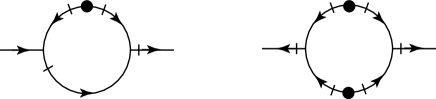
FIG. 1.: The one-loop diagrams contributing to the renormalization of (left) $D_{\|}$ and (right) $M_{\|}$. The legs with the outgoing arrow are for the response fields $(\tilde{\alpha},\tilde{\beta})$ and the legs with the incoming arrow for the density fields $(\alpha,\beta)$. The bar denotes spatical differentiation and the dot an $M$ vertex.

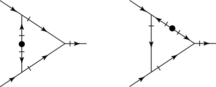
FIG. 2.: The one-loop diagrams contributing to the renormalization of $v$. These two diagrams cancel each other.

The dynamical exponent is given by $z=2$, leaving $D_{\perp}$ and $M_{\perp}$ unchanged under the RG flow. The flow equations for $D_{\|}$ and $M_{\|}$ have the same contribution and the ratio $D_{\|}/M_{\|}$ remains constant $(=1)$. The reaction rate $\lambda$ is renormalized only by the $\lambda$ terms, not the drift term. Combining the flow equations for $D_{\perp}$, $D_{\|}$, and $v$, we find the flow equation for the expansion parameter $g$:

$$\frac{d\ln g}{dl}=(2-d)-\frac{3}{4}g.$$ (28)

For $d>d_{c}=2$ we find an infrared stable fixed point $g^{*}=0$, and in a region of attraction, $D_{\|}$ and $M_{\|}$ remain constant. The scaling form of the average concentration of $A$ and $B$ particles [$c(t)\equiv c_{A}(t)=c_{B}(t)$][8]

$$c(t)=e^{-d\ell}\left({n_{0}(\ell)\over 8\pi^{2}D_{\|}(\ell)^{1/2}D_{\perp}(\ell)^{(d-1)/2}t(\ell)^{d/2}}\right)^{1/2},$$ (29)

gives $c(t)\sim t^{-d/4}$ using the time flow equation $t(\ell)=te^{-\int_{0}^{\ell}z(\ell)d\ell}$. Below the critical dimension $d_{c}$, there exists a nontrivial infrared stable fixed point at $g^{*}={4\over 3}\varepsilon$, and near this point $D_{\|}$ and $M_{\|}$ flow as $e^{2\epsilon\ell/3}$. Thus, the average concentration behaves as

$$c(t)\sim t^{-(d+1)/6}.$$ (30)

In summary, we have presented a systematic formalism to derive the field-theoretic action for systems of hard-core particles. Starting from the master equation for a stochastic process of the system, we have constructed the Fokker-Planck equation by introducing annihilation and creation operators with mixed commutation relations. This Fokker-Planck equation is connected to the stochastic differential equation by identifying the coefficient functions in the Itô interpretation. Finally, the stochastic differential equation is mapped onto field theory using the path integral, giving the field-theoretic action to be analyzed by the RG method.

Although there have been many attempts to incorporate the hard-core property of particles into field theory, our formalism has a very important advantage over other attempts. Our formalism can be applied to multispecies systems in arbitrary spatial dimension. As a paradigmatic example, we have applied our formalism to the $A+B\rightarrow\emptyset$ reaction-diffusion system with drift. Following straightforward steps to obtain the action and applying the momentum-shell RG method, we have calculated the long-time behavior for the average concentration of particles. Power counting shows that the upper critical dimension is $d_{c}=2$, and the drift term affects the RG flow only for fewer than two dimensions. Thus, for $d\geq 2$, the hard-core action behaves the same as the bosonic action derived by Lee and Cardy. The average concentration behaves as $t^{-1}$ for $d\geq 4$ and $t^{-d/4}$ for $4\geq d\geq 2$ in the long-time limits. Below the critical dimension, the drift term moves the stable fixed point to the non-trivial one and the average concentration behaves as $t^{-(d+1)/6}$ for $d\leq 2$. These results agree with the simulation results by Janowsky[10] and the scaling arguments by Ispolatov et al[11].

As mentioned before, our formalism has merit in extension to multispecies and to higher spatial dimensions. Also, it is necessary to use this formalism, not the bosonic formalism, when the system has nonvanishing concentrations in the steady states. The three-species reaction-diffusion system[12] and some other systems having nonvanishing steady states are under investigation using this formalism.

This research was supported by the KOSEF through Grand No. 981-0202-008-2.

REFERENCES

- [1]
- [2] See, for example, Nonequilibrium Statistical Mechanics in One Dimension, edited by V. Privman (Cambridge University Press, Cambridge, 1997).
- [3] See, for example, J. Marro and R. Dickman, Nonequilibrium Phase Transitions in Lattice Models (Cambridge University Press, Cambridge, 1999).
- [4] D. C. Mattis and M. L. Glasser, Rev. Mod. Phys. 70, 979 (1998), and references therein.
- [5] M. Doi, J. Phys. A 9, 1465 (1976); 9, 1479 (1976); P. Grassberger and M. Scheunert, Fortschr. Phys. 28, 547 (1980); L. Peliti, J. Phys. (Paris) 46, 1469 (1985).
- [6] B. P. Lee, J. Phys. A 27, 2633 (1994).
- [7] B. P. Lee and J. Cardy, J. Stat. Phys. 80, 971 (1995).
- [8] M. Deem and J.-M. Park, Phys. Rev. E 57, 2681 (1998).
- [9] J.-M. Park and M. Deem, Phys. Rev. E 57, 3618 (1998).
- [10] S. A. Janowsky, Phys. Rev. E 51, 1858 (1995); 52, 2535 (1995).
- [11] I. Ispolatov, P. L. Krapivsky, and S. Redner, Phys. Rev. E 52, 2540 (1995).
- [12] K. E. Bassler and D. A. Browne, Phys. Rev. E 55, 5225 (1997).
- [13] V. Brunel, K. Oerding, and F. van Wijland, e-print cond-mat/9911095.
- [14] P.-A. Bares and M. Mobilia, Phys. Rev. E 59, 1996 (1999).
- [15] D. ben-Avraham, V. Privman, and D. Zhong, Phys. Rev. E 52, 6889 (1995).
- [16] See, for example, K. Kawasaki, in Phase Transitions and Critical Phenomena, edited by C. Domb and M. S. Green (Academic Press, London, 1972), Vol. 2.
- [17] S.-C. Park, J.-M. Park, and D. Kim (unpublshed).
- [18] N. G. van Kampen, Stochastic Processes in Physics and Chemistry, enlarged ed. (Elsevier, Amsterdam, 1997).
- [19] P. C. Martin, E. D. Siggia, and H. A. Rose, Phys. Rev. A 8, 423 (1973).; J. Zinn-Justin, Quantum Field Theory and Critical Phenomena, 3rd ed. (Clarendon Press, Oxford, 1996).