Sequencing of folding events in Go-like proteins

I Introduction

Go-like models [1] provide minimal yet fairly realistic coarse-grained models of proteins. [2, 3] The main idea is to attach importance only to those aminoacid-aminoacid interactions which reside in the native contacts and then to choose the contact energies that minimize the total energy in the native conformation. This approach may seem to be overly simplistic but it generates models with fast kinetics of folding. In this sense, as noted by Takada [2], ”Go models may still be closer to reality than our current realistic models”. This is due to the fact that the presence of significant non-native interactions can overconstraint and thus frustrate a sequence of beads in continuum space [4]. Such a structural frustration is expected to be of small consequence in fully atomistic models that represent actual physical shapes of aminoacids. One may then say that Go-like models appear to provide a mutual compensation of two shortcomings in minimalistic models. A useful feature of the Go-like models is that they can be easily constructed to describe realistic protein structures. This ties well with the finding that the geometry of of the native state itself has crucial impact on the the foldability of proteins. [3, 5, 6, 7, 8]

Lattice (see e.g. Ref.[9]) and continuum space Go-like models have been studied in the literature. There are several versions of the continuum space Go models and they differ mostly in what kind of the contact potential is used and in whether any steric constraints are imposed or not. Among the interactions that have been considered there are: the square well potential,[10, 11] the Gaussian function,[12] the Lennard-Jones (LJ) potential [4, 13, 14, 15] and the short-range LJ-type potential with the exponents of 12 and 10 in the repulsive and attractive parts respectively.[16] It remains to be elucidated, however, which of these functional forms is the most adequate.

In a recent paper,[14] we have reported results of a study of several-sized $\alpha$-helices and $\beta$-sheets as modelled in the Go fashion. Our models employ the LJ potentials for the native contacts and the soft repulsive potentials for the non-native contacts. The latter are necessary to provide excluded volume and prevent entanglements. We have also considered models in which the steric constraints are taken into account. We have demonstrated that in all of these models of secondary structures the folding proceeds typically through well defined sequences of events which depend primarily on the geometry of the native conformation. This average order of events is robust when the conditions for folding are optimal but may become scrambled otherwise. The helices are found to fold preferably from the chain ends, whereas the $\beta$-hairpins usually fold by starting from the turn. Additionally, the formation of the contacts has been found to proceed faster in the final stages of folding. Such a sequencing of contacts in the $\beta$-hairpin formation resembles the kinetic zipping mechanism proposed in the literature [17, 18] and it agrees with recent simulations by Klimov and Thirumalai [15] and by Pande and Rokhsar.[19] The zipping mechanism has been found to dominate also in a model of the $\beta$-hairpin that contain a hydrophobic core (in which the interactions are stronger).[15] This indicates the important role played by the native geometry and it validates results obtained based on the Go model. Note, however, that the all-atom simulations by Dinner et al. [20] indicate existence of pathways in which the hydrophobic core is established first.

In the present study, we extend our Lennard-Jones based Go modelling [14] to several small globular proteins which incorporate both kinds of the secondary structures. The proteins that we consider are: a 46-monomer crambin (CRN), a 65-monomer chymotrypsin inhibitor 2 (CI2) and a 57-monomer Src Homology 3 domain of the fyn tyrosine-protein kinase (SH3). In order to simplify the analysis, we model these systems without implementation of the steric constraints. We demonstrate that our models form good folders.

Our main finding is that these models also generate a well defined average order in which contacts are established provided the temperature corresponds to optimal folding conditions. The folding history typically involves a steady establishment of successive contacts which is interspersed by several characteristic temporal gaps between certain stages.

Furthermore, we observe a good correlation between the separation of the contacts along the sequence and the average times of their first appearance during folding. Long-ranged contacts usually need much more time to get built than what the alpha helices need. This finding is consistent with recent experimental observation by Plaxco et al. [5] that the folding rates of proteins strongly depend on a contact order parameter which is determined from the average sequence separations between contacting residues in the native conformations. The correlation between the time needed to establish contacts and the sequence separation is obeyed in CRN in an almost perfect fashion. In CI2 and SH3, this correlation is disturbed but it remains strong. The idea that local interactions may dominate folding arose in studies of simple lattice models.[21] There are also, however, studies which attach importance to the nonlocal contacts.[22]

By examining the trajectories in details, we find that the typical sequencing of folding events, as extracted from the average times of establishing individual contacts, is the dominant folding scenario for all of the systems considered. In the case of crambin, for instance, we find that 83% of all trajectories follows the unique order of events. Such a high degree of determinism suggests that crambin may be considered as the single-route folder. For CI2 this degree of determinism is lower but remains high: about 70% of the trajectories follow the typical folding scenario. The typical sequencing of events for CI2 also has been found to be in agreement with experimental [23, 24] and other simulation [16, 25] results on the structure of the transition state. The trajectories for SH3 are found to be even more diversified with only 50% being typical. However, in 75% of the trajectories there is an early establishment of the $3_{10}$-helix and the distal loop hairpin which is consistent with experimental studies on the transition state. [26, 27, 28, 29, 30] We also find that in 90% of the trajectories the two $\beta$-sheets which are next to the distal loop and the so called RT loop (defined in Figure 11) are established earlier than the other segments. This is in good agreement with recent protein engineering analysis by Martinez and Serrano, [29] which indicates that the folding of SH3 seems to be composed of two folding subdomains.

The sequencing of the folding events is found not to depend on the viscous friction coefficient used in the simulations and moving the temperature away from the optimal value results in a ”scrambling” which is similar to that found in isolated secondary structures. Recently, there have been experimental studies [31, 32] which reported that a large amount of the solvent accessible surface area buried in the native state is also buried in the transition state for a wide range of concentration of a viscogenic agent. Studies by Ladurner and Fersht [33] suggest that the viscogenic agent stabilizes the native state and the transition state in parallel and to the same degree. Thus the folding mechanism appears not to depend on the solvent viscosity. The folding rate itself, on the other hand, has been reported to depend linearly on the solvent viscosity for some proteins by the isostability approach.[31, 32, 34]

In most of the present paper, the amplitude of the LJ native potentials is assumed to be fixed at a common value. However, we have also considered models in which certain contacts are made to be substantially stronger. Such contacts correspond to the disulfide bridges in crambin and to the hydrophobic contacts in the case of CI2 and SH3. We find that the strengthening of the contacts affects the time scales only marginally and the average sequencing order remains unchanged. This indicates that the sequencing of the contact formation is determined by the geometry of the native conformation. Our results are consistent with various experimental studies which suggests that the folding transition states are conserved among proteins which share the same overall native topology. [29, 35, 36]

The paper is organized as follows. In Section 2, we present a short description of the model and of the simulation method. In Section 3, we discuss ways to delineate the native basin and we determine the folding properties of the models. The mechanisms of folding for each of the proteins are discussed in Section 4. Section 5 provides conclusions.

II Models and Methods

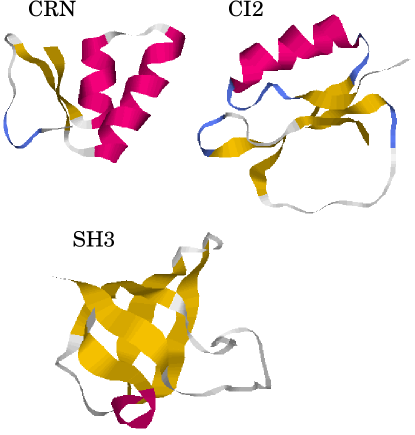
FIG. 1.: The native conformations of the proteins studied in the paper: crambin (CRN), chymotrypsin inhibitor 2 (CI2) and the SH3 domain (SH3). The PDB codes are 1crn, 2ci2 and 1efn.

We consider three single-domained globular proteins: CRN, CI2 and SH3. The ribbon plots of their native conformations are shown in Figure 1. The native conformations involve at least one alpha helix and at least two beta sheets in each case.

The proteins are modelled in a coarse-grained fashion, in which each amino acid is represented by a single bead located at the position of the C$\alpha$ atom. We adopt a simple Go-like interaction scheme and do not implement any the steric constraints.

The brief summary of our approach [14] is as follows. A chain conformation is defined by the set of position vectors $\{{\bf r}_{i}\}$, $i=1,2\ldots N$, where $N$ is then number of residues. The potential energy is assumed to take the form:

$$E_{p}(\{{\bf r}_{i}\})=\sum_{i=1}^{N-1}[k_{1}(r_{i,i+1}-d_{0})^{2}+k_{2}(r_{i,i+1}-d_{0})^{4}]$$ (1)

$$+\sum_{i+1<j}^{NAT}4\epsilon\left[\left(\frac{\sigma_{ij}}{r_{ij}}\right)^{12}-\left(\frac{\sigma_{ij}}{r_{ij}}\right)^{6}\right]$$ (2)

$$+\sum_{i+1<j}^{NON}4\epsilon\left[\left(\frac{\sigma_{0}}{r_{ij}}\right)^{12}-\left(\frac{\sigma_{0}}{r_{ij}}\right)^{6}+\frac{1}{4}\right]\Delta(r_{ij}-d_{nat}).$$ (3)

The first term in equation (1) represents rigidity of the backbone potential; $r_{i,i+1}$ is the distance between two consecutive beads; $d_{0}=3.8\AA$, $k_{1}=\epsilon$ and $k_{2}=100\epsilon$, where $\epsilon$ is the Lennard-Jones energy parameter corresponding to a native contact. The second term corresponds to interactions in the native contacts and the sum is taken over all pairs of residues $i$ and $j$ which form the native contacts in the target conformation. Two beads that are not consecutive in the sequence are assumed to form a native contact if their distance in the native conformation is less than 7.5$\AA$. $r_{ij}$ is the distance between two residues $i$ and $j$, and $\sigma_{ij}=2^{-1/6}\cdot d_{ij}$, where $d_{ij}$ is the corresponding native contact’s length. The third term represents the excluded volume interactions between monomers in the non-native contacts. We chose $d_{nat}=\left<d_{ij}\right>$ and $\sigma_{0}=2^{-1/6}\cdot d_{nat}$. $\Delta(r_{ij}-d_{nat})$ is a cut-off function which is equal to 1 for $r_{ij}\leq d_{nat}$ and 0 otherwise.

The proteins are studied by using molecular dynamics (MD) simulations in which the temperature control is accomplished through the Langevin noise term so that the equations of motion read

$$m\ddot{{\bf r}}=-\gamma\dot{{\bf r}}+F_{c}+\Gamma\;\;.$$ (4)

Here, ${\bf r}$ is a generalized coordinate of a bead, $m$ is the monomer mass, $F_{c}=-\nabla_{r}E_{p}$ is the conformation force, $\gamma$ is a friction coefficient and $\Gamma$ is the random force which is introduced to balance the energy dissipation caused by friction. $\Gamma$ is assumed to be drawn from the Gaussian distribution with the standard variance related to temperature, $T$, by

$$\left<\Gamma(0)\Gamma(t)\right>=2\gamma k_{B}T\delta(t),$$ (5)

where $k_{B}$ is the Boltzmann constant, $t$ denotes time and $\delta(t)$ is the Dirac delta function.

The equations of motion are integrated using the fifth order predictor-corrector scheme,[37] where the friction and random force terms appear as a noise perturbing the motion at each integration step. The integration time steps are taken to be $\Delta t=0.005\tau$ apart, where $\tau=\sqrt{ma^{2}/\epsilon}$ is a characteristic oscillatory time unit. The characteristic length $a$ is chosen to be equal to $5\AA$, which is a typical value of the Van der Waals radius of the amino acid residues. The simulations are performed with two values of the friction coefficient $\gamma$: $2m/\tau$, which is a typical choice in the MD simulations of liquids, and $10m/\tau$ which we used before.[14] We have already demonstrated that when $\gamma$ is larger than $1m/\tau$ the folding times scale linearly with $\gamma$. Here, we show (in Section 4A) that the ordering of the events is not affected by the value of $\gamma$, at least in the case of CRN, so in the remaining study we stay with $\gamma=2m/\tau$ to reduce the usage of the cpu. It should be noted that the realistic $\gamma$ for amino acids in a water solution has been argued [38] to be of order $50m/\tau$. In the following, the temperature will be measured in the reduced units of $\epsilon/k_{B}$.

III Folding properties

Proteins found in nature differ from random heteropolymers in that their native states are not only thermodynamically stable but are also easily accessible kinetically under the physiological conditions. A kinetic criterion [39] for a sequence to be a good folder (and thus to be a good model of a protein) is that the folding temperature, $T_{f}$, which characterizes the thermodynamical stability, is larger than the glass transition temperature $T_{g}$. However, there are problems with the definition of $T_{g}$: it depends on the value of an arbitrary cutoff time and, more importantly, it presupposes existence of the glassy phase. A natural alternative is to use the temperature, $T_{min}$,[40] at which folding is the fastest, as a reference temperature. The bad folders are then those for which $T_{f}$ is significantly lower than $T_{min}$. An alternative equilibrium criterion, on the other hand, specifies that good foldability arises when the folding temperature $T_{f}$ is close to the collapse transition temperature $T_{\theta}$.[41, 42]

In lattice models, the native state usually consists of just a single microstate which simplifies determination of $T_{f}$ and of the folding times. $T_{f}$ is typically defined as a temperature at which the probability of being in the native state crosses $\frac{1}{2}$. In the off-lattice models, any conformation is of measure zero and the native conformation has to be considered together with its immediate neighborhood. A shape distortion method for calculation of the size of a native basin has been recently proposed by Li and Cieplak.[13] The idea is to monitor the time dependence of the characteristic conformational distance $\delta$ away from the native state based on many short unfolding trajectories that evolve at different temperatures. $\delta$ is given by

$$\delta^{2}=\frac{2}{N^{2}-3N+2}\sum_{i=1}^{N-2}\sum_{j=i+2}^{N}(r_{ij}-r_{ij}^{NAT})^{2},$$ (6)

where $r_{ij}$ and $r_{ij}^{NAT}$ are the monomer to monomer distances in the given conformation and in the native state respectively. The distance $\delta$ is measured in $\AA$. At a sufficiently large time scale the conformational distance saturates below some critical temperature, $T_{c}$. The saturation value of the distance at this temperature, $\delta_{c}$, is used for the estimated native basin’s size. Additionally, $T_{c}$ has been found [13, 14] to be a measure of $T_{f}$.

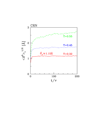
FIG. 2.: The average root mean square distance to the native state as a function of time for CRN. The results for each temperature are averaged over 400 trajectories that start from the native conformation.

Figure 2 illustrates the use of the shape distortion approach in the case of CRN. We considered 400 unfolding trajectories for each temperature and computed the average root mean square distance $\left<\delta^{2}\right>^{1/2}$ as function of time. The estimated basin size, $\delta_{c}=1.15\AA$, is obtained at $T_{c}=0.32$ which is the largest temperature at which the saturation is still observed. It should be noted that, in the case of crambin, however, a precise determination of $\delta_{c}$ and $T_{c}$ is not easy due to a broad borderline behavior. As shown in Figure 2, $T=0.45$ seems to be above $T_{c}$ because there is a small but steady increase of $\left<\delta^{2}\right>_{t}^{1/2}$ in time but the difference in the saturation or near-saturation levels of the curves is rather small. Thus the value of $\delta_{c}$ for CRN comes with a substantial error. In the case of CI2 (data not shown), the saturation is observed at $\delta_{c}$ of about $4\AA$. Such a large value of $\delta_{c}$ does not seem to be a realistic estimate of the basin size since it may correspond to not all native contacts being established. Thus the shape distortion method appears not to be reliable when more complicated structures than short chains are considered. We then simply declare $1.15\AA$, that we derived for crambin, to be a common approximate estimate of $\delta_{c}$ for the three sequences studied here.

An alternative way to define the native basin is through the number of the native contacts. In the following we assume that two monomers form a native contact if the distance between them is less than $1.5\sigma_{ij}$. Let $Q$ denote a fraction of the overlapping native contacts between the native state and a given conformation. $Q$=1 corresponds to a conformation that is in the native basin, whereas $Q$=0 to a fully non-overlapping conformation. It should be noted that the contact criterion is not always equivalent to the criterion which employs $\delta_{c}$. For instance, we have checked that there are conformations which have $\delta<\delta_{c}$ but $Q<1$ and there are also conformations which have $Q=1$ but $\delta>\delta_{c}$. This indicates a need for a more sophisticated multi-parameter description of the native basin.

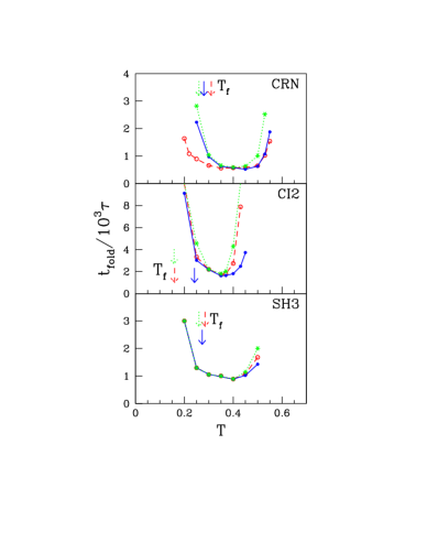
FIG. 3.: The temperature dependence of the median folding times for the model proteins using three different criteria to define the native basin: 1) $\delta<\delta_{c}$ (dashed line), 2) $Q$=1 (solid line) and 3) both $\delta<\delta_{c}$ and $Q$=1 (dotted line), where $Q$ denotes a fraction of the native contacts. The corresponding arrows indicate positions of $T_{f}$ and $T_{min}$.

We have computed $T_{f}$ and the temperature dependence of the folding times for the three model proteins studied here using three criteria for what constitutes the native basin. These are: 1) $\delta<\delta_{c}$, 2) $Q$=1, and 3) both $\delta<\delta_{c}$ and $Q$=1 which is the most stringent criterion. The median folding time at each $T$ are obtained based on typically 200 folding trajectories which start from random unfolded conformations. The starting conformations are generated by performing self-avoiding walks with randomly chosen bond angles and dihedral angles. The bond angles are additionally restricted to be drawn form the [$0$, $\pi/2$] interval in order to make the conformations be shaped in an unfolded way. $T_{f}$’s are calculated based on 10 to 15 long $MD$ trajectories at equilibrium at various temperatures. The trajectories start from the native state and last from $5\times 10^{4}\tau$ to $10^{5}\tau$ depending on the system size. The first few thousands $\tau$’s are reserved for equilibration and are not included in the averaging process.

Figure 3 shows that the median folding times follow the usual $U$-shape dependence on temperature. For all cases, one observes that the folding times at $T_{min}$ and $T_{min}$ itself do not depend on the criteria used to define the native basin. Away from $T_{min}$, the three criteria work differently in each protein and the third criterion yields the narrowest U shape. A similar statement holds for $T_{f}$ and the most stringent criterion yields the lowest value of $T_{f}$. Note, however, that overall the three criteria give similar values of $T_{f}$ and in practice can be used interchangeably, especially in the case of CRN and SH3. In the case of CI2, the difference between the $\delta_{c}$-based criterion and the contact-based criterion is the largest. We think that this large difference is due to the presence of the active-site loop (shown in Figure 10) which is poorly coupled to the rest of the structure.

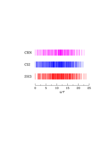
FIG. 4.: The phononic spectra of the studied proteins. The values of $\omega_{1}\tau$ given in radians are, top to bottom: 0.76, 0.51, 1.15

For the three model proteins studied here we observe that $T_{f}$’s are comparable to $T_{min}$’s but are generally lower. Note that at temperatures around $T_{f}$ the native state can still be reached within a time scale that is only about several times longer than the folding time at $T_{min}$. Thus the sequences we study can still be considered to be good or at least fair folders. SH3 appears to be the best folder of the three systems and CI2 to be the worst. Note that if one defines the glass transition temperature $T_{g}$ as one at which the folding times become a few orders of magnitude longer (say, 1000 times) than the folding time at $T_{min}$, then for all of the three models $T_{f}$ is larger than $T_{g}$.

We have shown before [14] that phononic spectra for vibrations around the native state offer some clues about the stability of proteins: the bigger the gap in the low end frequency spectrum, the bigger the mechanical stability, which should correlate with a bigger value of $T_{f}$. We repeat the calculation of the phononic spectra for our model proteins. The procedure involves diagonalization of a $3N\times 3N$ matrix of the elastic constants.[43] The elastic constants are calculated numerically as the second derivatives of the potential energy taken at the native conformation. When calculating an elastic constant for a bead we freeze all the remaining beads and measure the resulting increase in the force when the unfrozen bead is displaced along a given Cartesian direction. The diagonalization is done with the use of the Jacobi transformation method.[44] The resulting phononic spectra are shown in Figure 4. The frequencies $\omega$ are measured in units of $\tau^{-1}$. In each spectrum there are six zero frequency modes which correspond to the translational and rotational degrees of freedom of the whole system. The lowest non-zero frequency $\omega_{1}$ (which define the gaps in the spectra) corresponds to the first excited mode. For CRN, CI2 and SH3 $\omega_{1}$’s are found to be equal to 0.76$/\tau$, 0.51$/\tau$ and 1.15$/\tau$ respectively. Notice that CI2 which has the lowest $\omega_{1}$ is indeed the system with the lowest $T_{f}$. For CRN and SH3, however, the $T_{f}$’s are comparable but $\omega_{1}$ for CRN is somewhat smaller than for SH3. Thus the correlation between $\omega_{1}$ and $T_{f}$ is not strong. Note that $\omega_{1}$ which is a direct measure of mechanical stability which should provide bounds against melting of the native conformation. The stability measured by $T_{f}$ is instead also a measure of the role of the non-native energy valleys — can their presence reduce the probability of the sequence staying in the native valley.

IV Folding mechanism

We now discuss the order of folding events in the three model proteins. The simplified character of the model allows us to consider hundreds of folding trajectories and to monitor individual contacts. We focus on the native contacts and ask what are the characteristic times $t_{0}$’s at which particular contacts are established if one starts from an unfolded conformation. In $\alpha$-helices and $\beta$-structures the contacts were found to be getting established in a well defined order [14] and we seek to find out if the same holds in the case of larger sequences.

A Crambin (CRN)

Crambin (CRN) is a small globular protein with only 46 amino acids. Because of its small size, it has been a subject of many early MD simulations (see e.g. Ref.[45]). The native structure of CRN exhibits a rich amount of the secondary structures. There are two $\alpha$-helices which are packed together with two short $\beta$-strands, as shown in the bottom of Figure 4. The structure is additionally stabilized by three disulfide bridges (Cys3 - Cys40, Cys4 - Cys32 and Cys16 - Cys26) which improve the thermodynamic stability significantly.

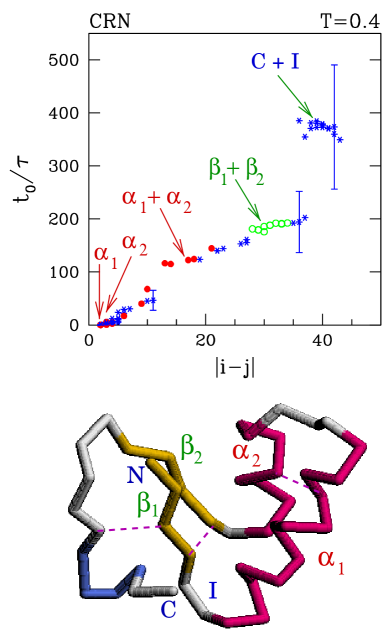
FIG. 5.: Top: the average times $t_{0}$’s needed to establish contacts for the first time during folding for CRN at $T$=$T_{min}$=0.4. The times are plotted against the sequence separations, $|i-j|$, between the monomers that form the contacts. The error bars indicate the dispersions in the values of $t_{0}$’s. The error bars generally grow with $t_{0}$ and several characteristic values are shown as an illustration. The contacts are grouped into three categories: 1) those which belong to the $\alpha$-helices (solid circles), 2) those which belong to the $\beta$-sheets (open circles) and 3) other (starred marks). Bottom: the native conformation of CRN in which the various secondary structures are indicated. N and C denote the N- and C-termini of the chain respectively. I denotes a segment which connects the $\beta_{1}$-strand to the helix $\alpha_{1}$. The dashed lines indicate the positions of the disulfide bridges.

We first discuss the case of $\gamma=2m/\tau$. Figure 5 shows the contact’s establishment times $t_{0}$’s for CRN as calculated at $T$=$T_{min}$=0.4. The averages are taken over 400 independent folding trajectories that start from random unfolded conformations. The times are plotted against the sequence separation of the contacting residues, denoted as $|i-j|$. The error bars shown at selected data points indicate the dispersions of these times. One can easily notice a strong correlation between the $t_{0}$’s and the values of $|i-j|$. The local contacts, i.e. the contacts with $|i-j|$ equal to 2 or 3, are formed almost immediately. The bigger the sequential separation, the longer the average time that is needed for a contact to start contributing to the energy. One can also observe a gap in $t_{0}$’s between a group of contacts with the largest sequence separations and the rest of the contacts. The big error bars shown for some contacts indicate that the times and magnitudes of the gaps vary substantially among the trajectories so it is simplest to start our discussion by considering the average sequencing of events.

In order to understand the formation of the secondary structures better we have divided the contacts into three groups: 1) the contacts that are present in the $\alpha$-helices or link neighboring helices; 2) the contacts that are formed between the $\beta$-strands and 3) other contacts, i.e. which belong to the coils, turns etc.

Figure 5 shows that contacts that belong to the helix group are formed the earliest, are all established within 150$\tau$, and remain locked afterwards. The contacts from the second group appear almost simultaneously at about 200$\tau$, whereas the members of third group become established at various time scales. Notice that the tertiary contacts between two helices are formed slower than within single helices but faster than between the $\beta$-strands. As shown in Figure 5, the typical folding scenario is as follows. First, the $\alpha$-helices are established, then the two helices are locked together. Next, the contacts between the $\beta$-strands 1 and 2 are established. At this stage, there is a long temporal gap and finally the C-terminus gets connected to the rest of the structure which is almost folded.

We now consider the case of $\gamma$ which is 5 times larger. Figure 6a shows that the increase in $\gamma$ results in a five-fold elongation of the characteristic times but the sequencing of the contacts is not affected. The pattern shown in Figure 6a is almost identical to that shown in Figure 5. This is in agreement with recent experimental studies [31, 32, 33, 34] which suggested that the folding mechanism does not seem to depend on the solvent viscosity.

Figure 6b illustrates what happens if $T$ is changed from $T_{min}$ to a lower value of 0.25. The value of $\gamma$ is the same as in Figure 5: $2m/\tau$. The change in the temperature increases the scatter in the sequencing but the typical folding history remains unchanged. A similar observation holds also for temperatures which are higher than $T_{min}$ (but are not too high).

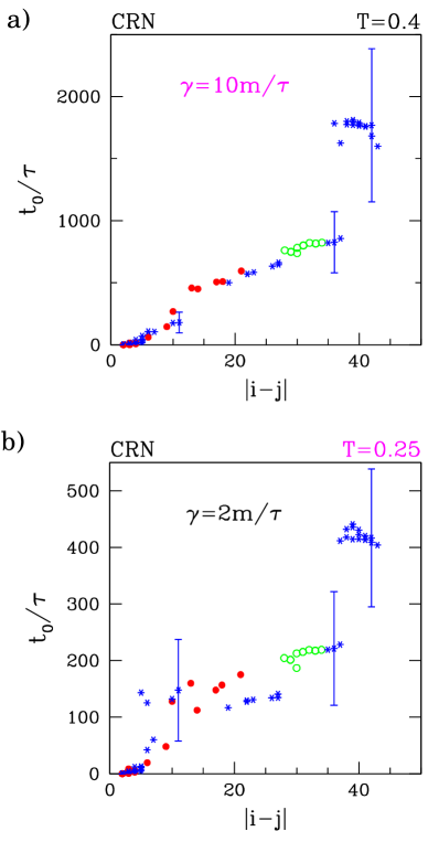
FIG. 6.: Same as the top of Figure 5, but a) for $\gamma=10m/\tau$ and b) for $T=0.25$, a temperature somewhat lower than $T_{min}$.

Results shown in Figures 5 and 6 have been obtained by averaging over many trajectories. Figure 7 shows a single typical folding trajectory for CRN at $T$=0.4 and $\gamma=2m/\tau$, which exhibits a temporal gap in the folding history as measured by the contact establishment times. The top of the figure shows $t_{0}$’s and the bottom shows the corresponding evolution in $Q$, $E_{p}$, and the radius of gyration, $R_{g}$. The potential energy is seen to drift downhill and $R_{g}$ gets shrinked. $Q$ first increases monotonically but then it merely oscillates for a period of about 300$\tau$ before entering the vicinity of $Q$=1. This period corresponds to the gap and is indicated by the arrow.

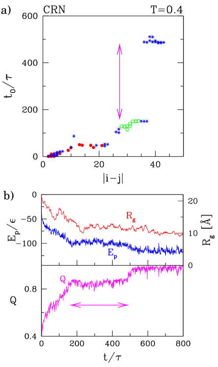
FIG. 7.: An example of a folding trajectory of CRN at $T=T_{min}=0.4$. Top: the contact establishment times $t_{0}$’s versus the sequence separation $|i-j|$. Bottom: the time dependence of the potential energy $E_{p}$, the radius of gyration $R_{g}$, and the fraction of the native contacts $Q$.

Figure 8 shows selected conformations that appear on the trajectory shown in Figure 7. It illustrates the folding scenario described in Figure 5. The trajectory starts from a random unfolded conformation at $t=0\tau$. At $t=80\tau$ one can observe the two helices are packed together to form a bundle. Then the $\beta$-sheets appear as shown at $t=160\tau$. At this moment there is one chain terminus that is still far apart from the rest of the chain. It takes a significant amount of time of about 330$\tau$ (corresponding to the gap in $t_{0}$’s) for this terminus to move to its proper destination in the native conformation. The last contacts start to form at $t\approx 490\tau$ and finally the chain acquires its native shape, when all of the contacts are established. This happens at $t=599\tau$.

FIG. 8.: Examples of conformations probed from the trajectory shown in Figure 7.

It should be noticed that the folding scenario presented above is just the most likely scenario and it follows from the geometry of the native conformations. There can be other trajectories with a different sequencing of events, depending on the initial conditions. For instance the C-terminus may be attached to the fragment I before the $\beta_{1}$–$\beta_{2}$ sheet is formed. In order to check the role of the other scenarios we have examined 100 trajectories in details. We find that among them there are:

• 83 trajectories with the scenario:
  $\alpha_{1}+\alpha_{2}\longrightarrow\beta_{1}+\beta_{2}\longrightarrow C+I$,

• 9 trajectories with the scenario:
  $\alpha_{1}+\alpha_{2}\longrightarrow C+I\longrightarrow\beta_{1}+\beta_{2}$,

• 5 trajectories with the scenario:
  $C+I\longrightarrow\alpha_{1}+\alpha_{2}\longrightarrow\beta_{1}+\beta_{2}$,

• 3 trajectories with the scenario:
  $\beta_{1}+\beta_{2}\longrightarrow\alpha_{1}+\alpha_{2}\longrightarrow C+I$.

We observe that the folding scenario presented by the average sequencing of contacts is clearly dominating.

In the discussion above all of the native contacts had the same amplitude $\epsilon$ in the LJ potentials. It is interesting to ask what would happen if the amplitudes were not uniform. Specifically, the interactions corresponding to the disulfide bridges are expected to be significantly stronger and we ask if this could affect the folding events. There are three disulfide bridges in crambin, as indicated in Figure 5. Figure 9 shows the results on the event sequencing when the interactions in the bridges is made five times stronger. One can notice that the characteristic times and the gap become somewhat smaller but the essential physics of the sequencing does not change. Thus the sequencing is primarily determined by the topology of the native conformation.

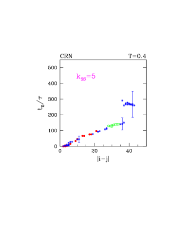
FIG. 9.: The sequencing of the contacts for CRN, at $T=0.4$ in the case in which the amplitudes of the potentials corresponding to the disulfide bonds are five times larger than for the other native contacts.

B Chymotrypsin Inhibitor 2 (CI2)

In crambin, the order of events is perfectly correlated with the sequence separation of the couplings. This is not so in the two other systems although the degree of such correlations remains high. From now on we work only with $\gamma=2m/\tau$.

We now consider CI2 which is a 83-residue protein. The first 18 residues are not resolved by either x-ray crystallography or NMR, and are considered to be irrelevant in protein engineering experiments since they do not contribute to the stability or functionality of the protein. The remaining 65 residues form a well-known native conformation in which an $\alpha$-helix is packed against four $\beta$-strands. Experimental results show that CI2 folds rapidly by a two-state mechanism.[23, 24]

In the present study, we examine the folding mechanism of CI2 along the same lines as it has been done for CRN in the last section. Figure 10 shows the contact establishment times for CI2 obtained at its temperature of the fastest folding — $T_{min}=0.35$. Similar to CRN, there is a clear dependence of the average $t_{0}$’s on the sequence separation of the contacts, although this dependence is less perfect. The $\alpha$-helix is formed rapidly while the $\beta$-sheets are established at various time scales. The folding scenario, on an average, can be presented as follows. After the $\alpha$-helix is formed the $\beta$-sheet between two strands $\beta_{3}$ and $\beta_{4}$ is also established. Then, it takes about 800$\tau$ for the sheet between $\beta_{2}$ and $\beta_{3}$ to start to form. Interactions between strands $\beta_{1}$ and $\beta_{4}$ appear at the last stage of folding. This happens just after several long range contacts between the chain’s segment connecting strand $\beta_{1}$ and helix $\alpha$ (labeled by $I_{1}$ in Figure 10) and the coil fragment connecting strands $\beta_{3}$ and $\beta_{4}$ (labeled by $I_{2}$) are established. There are two characteristic gaps in the time scales. The first one is between the the $\beta_{3}$-$\beta_{4}$ interaction and the $\beta_{2}$-$\beta_{3}$ interaction. The second one is between the $\beta_{2}$-$\beta_{3}$ and the $\beta_{1}$-$\beta_{4}$ interaction.

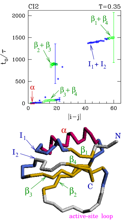
FIG. 10.: The same like Figure 5, but for CI2, at $T$=0.35.

Then we examine 100 trajectories and find that there are:

• 69 trajectories with the scenario:
  $\beta_{3}+\beta_{4}\longrightarrow\beta_{2}+\beta_{3}\longrightarrow\beta_{1}+\beta_{4}$,

• 15 trajectories with the scenario:
  $\beta_{2}+\beta_{3}\longrightarrow\beta_{3}+\beta_{4}\longrightarrow\beta_{1}+\beta_{4}$,

• 15 trajectories with the scenario:
  $\beta_{3}+\beta_{4}\longrightarrow\beta_{1}+\beta_{4}\longrightarrow\beta_{2}+\beta_{3}$,

• 1 trajectories with the scenario:
  $\beta_{1}+\beta_{4}\longrightarrow\beta_{3}+\beta_{4}\longrightarrow\beta_{2}+\beta_{3}$.

Notice that for CI2 the trajectories are more diversified than in the case of CRN — the CI2 is a larger system. The folding scenario corresponding to the average sequencing of contacts still dominates.

Experimental [24] studies on CI2 have indicated that the transition state ensemble of CI2 is broad. It means that there exist many pathways to the native state and none of them is dominant, which supports a “new view” of the protein folding.[46] Our present analysis shows that there is a dominant sequencing of events among the pathways — at least when the events are measured in terms of what contacts are established. Note, however, that a given sequencing may still correspond to multiple pathways. The sequencing of events found in CI2 is less pronounced compared to CRN. Thus, our results are not in disagreement with the experimental results. Studies on the structure of the transition state [16, 24, 25] have indicated that in the transition state the $\beta_{1}$-strand and the $\alpha$-helix interact weakly with the rest of the structure. This observation also seems to be consistent with our calculations on the sequencing. As it has been shown, the last folding event usually involves establishing the contacts between the part of the protein which spans from the N-terminus to the $\alpha$-helix and the rest of the structure. This latest rearrangement is also found to be consistent with the unfolding simulations for the full-atom model of CI2 [25] if we assume that that unfolding corresponds to a reversed sequencing of the events.

In order to examine the influence of the hydrophobic core on the sequencing of the events, we have studied what happens when strengths of 8 contacts between the hydrophobic residues (Val28 - Ile76, Val28 - Val79, Val32 - Ile76, Ile48 - Val66, Val50 - Leu68, Val66 - Val82, Val70 - Ile76, Ile76 - Val79) are made stronger by the factor of 5. We find that the average sequencing is affected very little. The changes are even smaller than in the case of CRN when the disulfide bonds are made stronger.

C SH3 domain (SH3)

There are a number of the Src Homology 3 (SH3) domains which all fold to the same native conformation by a two-state mechanism: src,[26] $\alpha$-spectrin,[27, 28, 29] fyn tyrosine kinase [47] and phosphatidylinositol 3 -kinase (PI3-kinase).[48] Since the difference between the native conformations of these domains are small, we will concentrate on the SH3 domain of the fyn tyrosine kinase (PDB code: 1efn; residues 85-141). The structure of this 57-residue peptide fragment is shown in Figure 1 and 11 (bottom). It has one small $3_{10}$-helix and five $\beta$-strands which are packed together to form a $\beta$-sandwich. The $\Phi$-value analysis of the fyn SH3 domain has been reported recently,[35] after it was done for the two other homologies: src [26] and $\alpha$-spectrin.[27, 28] In contrast to CI2, the transition state of SH3 is found to be highly polarized. This term means that there exists a dominant route to the native state which has a significantly lower free energy than all other routes.

The sequencing of the contacts for SH3 at $T_{min}$ of 0.4 is presented in Figure 11. One can observe a much weaker dependence of $t_{0}$’s on the sequence separation of the contacts than in the case of CRN and CI2. The most distant contacts are established much earlier than some middle range tertiary contacts. The most possible folding scenario is found to be as follows. After the $3_{1}0$-helix is established, the $\beta$-hairpin of the distal loop is also formed immediately afterwards. At the same time, the contacts within the RT loop start to become established which leads to the formation of the sheet between the $\beta_{1}$ and $\beta_{2}$ strands. These above structures are established within 100$\tau$, on the average. Their further rearrangement requires much longer time. The $\beta_{5}$-strand starts to interact with the $\beta_{1}$-strand at about 500$\tau$. Most of the contacts that form the sandwich are also established at this time. The latest rearrangement, which appears to happen between fragment L of the RT loop and strand $\beta_{4}$, occurs at about 1000$\tau$ and this accomplishes the folding.

Among 100 of the trajectories there are:

• 50 trajectories with scenario:
  $\beta_{3}+\beta_{4}\longrightarrow\beta_{1}+\beta_{2}\longrightarrow\beta_{1}+\beta_{5}\longrightarrow L+\beta_{4}$,

• 25 trajectories with scenario:
  $\beta_{3}+\beta_{4}\longrightarrow\beta_{1}+\beta_{2}\longrightarrow L+\beta_{4}\longrightarrow\beta_{1}+\beta_{5}$,

• 8 trajectories with scenario:
  $\beta_{1}+\beta_{2}\longrightarrow\beta_{3}+\beta_{4}\longrightarrow\beta_{1}+\beta_{5}\longrightarrow L+\beta_{4}$,

• 7 trajectories with scenario:
  $\beta_{1}+\beta_{2}\longrightarrow\beta_{3}+\beta_{4}\longrightarrow L+\beta_{4}\longrightarrow\beta_{1}+\beta_{5}$,

• 10 trajectories with other possible sequencings (not more than 2 for each scenario).

One can notice that the sequencings among trajectories seem to be more diversified than in the case of CI2. The folding mechanism presented by the average sequencing of contacts still dominates but only half of the trajectories fold exactly according to this scenario. However, in 75 out of 100 trajectories, the $\beta_{3}$-$\beta_{4}$ sheet is formed earlier than the other segments. This appears to be in very good agreement with numerous experimental studies [26, 27, 28, 29, 30, 35] which reported that the distal loop hairpin is clearly present in the transition state. Notice also that in 90 out of 100 trajectories the $\beta_{1}$-$\beta_{2}$ and $\beta_{3}$-$\beta_{4}$ sheets are formed before the $\beta_{1}$-$\beta_{5}$ sheet and the $L$-$\beta_{4}$ contacts are established. This is consistent with a recent $\Phi$-value analysis by Martinez and Serrano [29], which suggests that the folding of SH3 seems to be composed of two folding subdomains. One of such domain consists of the $3_{10}$-helix and the distal loop hairpin, while the other corresponds to the RT loop.

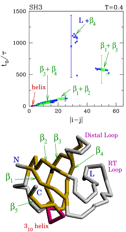
FIG. 11.: The same like Figure 5, but for SH3, at $T$=0.4.

Like for CI2 we have checked that increasing (by a factor of 5) the strengths of the contacts in the hydrophobic core does not lead to any significant change in the sequencing. For SH3, our chosen contacts that correspond to the hydrophobic core are Leu86 - Ile111, Leu101 - Ile133, Ile111 - Glu121 and Glu121 - Ile133. Experimentally, it has been shown [28] that certain mutations in the $\alpha$-spectrin SH3 can significantly increase both thermodynamic stability and folding rates without affecting transition states. The structure of the transition state has also been shown to be highly conserved among the SH3 homologies. [29, 30, 35] This indicates that the folding mechanism of SH3 depends primarily on the native topology instead of on the specific interactions. Thus our simulation results with increasing the hydrophobic interactions are consistent with those experimental findings.

V Conclusions

In summary, we have studied three globular proteins in the Go-like models with the Lennard-Jones potentials for the native contacts. We have delineated the native basins of the models by several (contact and distance based) criteria which were found to be almost equivalent in practice. The models were found to be stable and well folding. We have found that there is a strong correlation between the time to form a contact and its corresponding distance along the sequence. This is consistent with recent observation by Plaxco et al. [5] on the dependence of the folding rates on the contact order parameters of the native states. In general, the $\alpha$-helices which are stabilized mainly by the local contacts appear much faster than the $\beta$-sheets. History of folding contains several gaps when folding is hampered temporarily. Usually, trajectories which evolve according to the average scenario are the most frequent kind of possible trajectories. The folding scenarios are found to be in agreement with studies on the structure of the transition states.

We also find that the average sequencing of the folding events does not depend on the viscosity of the environment. Furthermore, large changes in the strength of certain contact energies or small changes in the temperature affect the sequencing very little. All this indicates that the folding evolution depends primarily on the geometry of the native conformation.

We are grateful to Jayanth R. Banavar for useful discussions. This work was supported by Komitet Badan Naukowych (Poland; Grant Number 2P03B-025-13). Figures 1, 5, 8, 10 and 11 are prepared with the help of the program RasMol version 2.6.

REFERENCES

- [1] N. Go, Macromolecules 9, 535 (1976); N. Go, and H. Abe, Biopolymers 20, 991 (1981).
- [2] S. Takada, Proc. Natl. Acad. Sci. USA 96, 11698 (1999).
- [3] E. Alm, and D. Baker, Curr. Opi. Struct. Biol. 9, 189 (1999).
- [4] M. S. Li and M. Cieplak, Phys. Rev. E 59, 970 (1999).
- [5] K. W. Plaxco, K. T. Simons, and D. Baker, J. Mol. Biol. 277, 985 (1998).
- [6] P. G. Wolynes, Proc. Natl. Acad. Sci. USA 93, 14249 (1996).
- [7] C. Micheletti, J. R. Banavar, A. Maritan, and F. Seno, Phys. Rev. Lett. 82, 3372 (1999).
- [8] A. Maritan, C. Micheletti, and J. R. Banavar, Phys. Rev. Lett. 84, 3009 (2000).
- [9] M. Cieplak, T. X. Hoang, and M. S. Li, Phys. Rev. Lett. 83, 1684 (1999).
- [10] Y. Zhou and M. Karplus, Nature 401, 400 (1999).
- [11] N. V. Dokholyan, S. V. Buldyrev, H. E. Stanley, and E. I. Shakhnovich, Folding Des. 3, 577 (1998);
- [12] C. Hardin, Z. Luthey-Schulten, and P. G. Wolynes, Proteins: Struct, Funct., Genet. 34, 281 (1999).
- [13] M. S. Li and M. Cieplak, J. Phys. A 32, 5577 (1999).
- [14] T. X. Hoang, and M. Cieplak, J. Chem. Phys. 112, 6851 (2000).
- [15] D. K. Klimov, and D. Thirumalai, Proc. Natl. Acad. Sci. USA 97, 2544 (2000).
- [16] C. Clementi, H. Nymeyer, and J. N. Onuchic, J. Mol. Biol. 298, 937-953 (2000).
- [17] K. A. Dill, K. M. Fiebig, and H. S. Chan, Proc. Natl. Acad. Sci. USA 90, 1942 (1993).
- [18] V. Munoz, P. A. Thompson, J. Hofrichter, and W. A. Eaton, Nature 390, 196 (1997).
- [19] V. S. Pande, and D. S. Rokhsar, Proc. Natl. Acad. Sci. USA 96, 9062 (1999).
- [20] A. R. Dinner, T. Lazaridis, and M. Karplus, Proc. Natl. Acad. Sci USA 96, 9068 (1999).
- [21] R. Unger, and J. Moult, J. Mol. Biol. 259, 988 (1996).
- [22] V. I. Abkevich, A. M. Gutin, and E. I. Shakhnovich, J. Mol. Biol. 252, 460 (1995).
- [23] S. E. Jackson and A. R. Fersht, Biochem. 30, 10428 (1991).
- [24] S. E. Jackson, M. Moracci, N. ElMasry, C. M. Johnson and A. R. Fersht, Biochem. 32, 11259 (1993).
- [25] A. Li, and V. Daggett, Proc. Natl. Acad. Sci. USA 91, 10430 (1994).
- [26] V. P. Grantcharova, D. S. Riddle, J. V. Santiago, and D. Baker, Nat. Struct. Biol. 5, 714 (1998).
- [27] A. R. Viguera, L. Serrano, and M. Wilmanns, Nat. Struct. Biol. 3, 874 (1996);
- [28] J. C. Martinez, M. T. Pisabarro, and L. Serrano, Nat. Struct. Biol. 5, 721 (1998).
- [29] J. C. Martinez, L. Serrano, Nat. Struct. Biol. 6, 1010 (1999).
- [30] D. S. Riddle, V. P. Grantcharova, J. V. Santiago, E. Alm, I. Ruczinski, and D. Baker, Nat. Struct. Biol. 6, 1016 (1999).
- [31] M. Jacob, T. Schindler, J. Balbach, and F. X. Schmid, Proc. Natl. Acad. Sci USA 94, 5622 (1997).
- [32] K. W. Plaxco, and D. Baker, Proc. Natl. Acad. Sci USA 95, 13591 (1998).
- [33] A. G. Ladurner, and A. R. Fersht, Nat. Struct. Biol. 6, 28 (1999).
- [34] R. P. Bhattachryya, and T. R. Sosnick, Biochemistry 38, 2601 (1999).
- [35] K. W. Plaxco, S. Larson, I. Ruczinski, D. S. Riddle, E. C. Thayer, B. Buchwitz, A. R. Davidson, and D. Baker, J. Mol. Biol. 298, 303 (2000).
- [36] F. Chiti, N. Taddei, P. M. White, M. Bucciantini, F. Magherini, M. Stefani, and C. M. Dobson, Nat. Struct. Biol. 6, 1005 (1999).
- [37] M. P. Allen and D. J. Tildesley, Computer Simulation of Liquids (Oxford University Press, New York, 1987).
- [38] D. K. Klimov, and D. Thirumalai, Phys. Rev. Lett. 79, 317 (1997).
- [39] N. D. Socci and J. N. Onuchic, J. Chem. Phys. bf 101, 1519 (1994); See also M. Cieplak and J. R. Banavar, Folding Des. 2, 235 (1997).
- [40] M. Cieplak, M. Henkel, J. Karbowski, and J. R. Banavar, Phys. Rev. Lett. 80, 3654 (1998); M. Cieplak and T. X. Hoang, Phys. Rev. E 58, 3589 (1998).
- [41] C. J. Camacho, and D. Thirumalai, Proc. Natl. Acad. Sci USA 90, 6369 (1993).
- [42] D. K. Klimov and D. Thirumalai, Phys. Rev. Lett. 76, 4070 (1996).
- [43] J. Callaway, Quantum Theory of the Solid State, (Academic Press, New York and London, 1974).
- [44] W. H. Press, B. P. Flannery, S. A. Teukolsky, and W. T. Vetterling, Numerical Recipes in FORTRAN, (Cambridge University Press, Cambridge, 1993).
- [45] M. Karplus, Phys. Today 40, 68 (1987).
- [46] V. S. Pande, A. Y. Grosberg, T. Tanaka, and D. S. Rokhsar, Curr. Opin. Struct. Biol. 8, 68 (1998).
- [47] K. W. Plaxco, C. J. Morton, J. I. Guijarro, M. Pitkeathly, I. D. Campbell, and C. M. Dobson, Biochem. 37, 2529 (1998).
- [48] J. I. Guijarro, C. J. Morton, K. W. Plaxco, I. D. Campbell, and C. M. Dobson, J. Mol. Biol. 276, 657 (1998).