Out-of-equilibrium thermodynamic relations in systems with
aging and slow relaxation

Abstract

The experimental time scale dependence of thermodynamic relations in out-of-equilibrium systems with aging phenomena is investigated theoretically by using only aging properties of the two-time correlation functions and the generalized fluctuation-dissipation theorem (FDT). We show that there are two experimental time regimes characterized by different thermal properties. In the first regime where the waiting time is much longer than the measurement time, the principle of minimum work holds even though a system is out of equilibrium. In the second regime where both the measurement time and the waiting time are long, the thermal properties are completely different from properties in equilibrium. For the single-correlation-scale systems such as $p$-spin spherical spin-glasses, contrary to a fundamental assumption of thermodynamics, the work done in an infinitely slow operation depends on the path of change of the external field even when the waiting time is infinite. On the other hand, for the multi-correlation-scale systems such as Sherrington-Kirkpatrick model, the work done in an infinitely slow operation is independent of the path. Our results imply that in order to describe thermodynamic properties of systems with aging it is essential to consider the experimental time scales and history of a system as a state variable is necessary.

I INTRODUCTION

Glassy systems like spin-glasses and structural glasses below the glass transition temperatures are out of equilibrium even on the macroscopic time scale. Thus, the slow dynamics of glassy systems has been a subject of continuous interest in the past years [2]. Experimentally, the anomalous dynamical behaviors are characterized by slow relaxation with long time tail and aging phenomena.

Among them, aging phenomena are the most striking dynamical behaviors as follows: Two-time quantities like the correlation functions $C(t,t^{\prime})$ explicitly depend on the time elapsed after the quench $t^{\prime}$ (the waiting time). If the waiting time $t^{\prime}$ is of microscopic time scale, the phenomena are merely transient on the way of relaxation to equilibrium. However, dependence on the waiting time continues even when $t^{\prime}$ is so large that one-time quantities like the magnetization are asymptotically close to time-independent values [3]. Since these phenomena mean that the dynamics is not stationary, aging is a sign showing that these systems are out of equilibrium even in macroscopic time scale, i.e. several days or weeks.

These aging phenomena appear also in mean-field models of spin-glasses and do not disappear even in the infinite waiting time limit [4, 5]. In addition, the phase space of these models decomposes into a large number of areas separated with infinitely high free energy barriers. Thus, glassy systems never reach true equilibrium and hence they are beyond the scope of thermodynamics and equilibrium statistical mechanics. Hence, in order to describe thermodynamic properties of glassy systems, out-of-equilibrium thermodynamics based on a dynamical description without the assumption of ergodicity is necessary.

In investigation of such anomalous dynamical behavior of glassy systems, it was found that aging phenomena have some universal properties. Theoretical analyses have suggested that there are two time regimes characterized by different dynamical properties of the two-time correlation function $C(t,t^{\prime})$ and the associated linear response function $R(t,t^{\prime})$ [4, 5]. In the first time regime where the time difference $t-t^{\prime}$ is short compared to $t^{\prime}$, the dynamics looks stationary and the usual fluctuation-dissipation theorem (FDT) holds. On the other hand, in the second time regime where the time difference is comparable to $t^{\prime}$, aging phenomena occur, i.e. $C(t,t^{\prime})$ depends on $t^{\prime}$ apart from dependence on $t-t^{\prime}$. In addition, it is known that the usual FDT between the correlation $C(t,t^{\prime})$ and the response function $R(t,t^{\prime})$ should be modified in a well-defined way which involves the rescaling of the temperature [6]. The modification was found to be valid not only for mean-field models but also for other glassy systems: spin-glass models with finite-range interactions [7], real spin-glasses [8], structural glasses [9, 10, 11] and a model of phase separation [12]. In addition, it is known for some glassy systems that the correlation function $C(t,t^{\prime})$ obeys the scaling law that it depends on $t$ and $t^{\prime}$ only through the value of $\xi(t)/\xi(t^{\prime})$, where $\xi(t)$ is a system-dependent increasing function of time.

Aging of the correlation function and the modification of FDT imply that properties of the work done by modulating an external field in an isothermal process are completely different from properties predicted by traditional thermodynamics. In addition, the existence of the two time scales implies that thermodynamic properties must strongly depend on experimental time scales. Hence, the experimental time scale dependence of the thermodynamic properties of glassy systems should be investigated to construct out-of-equilibrium thermodynamics for glassy systems.

In order to describe our results precisely, we summarize thermodynamics for an isothermal process. Thermodynamics tells that when one quasistatically changes the external field the work needed for the change is independent of a path of changing the external field. In addition, the quasistatic work is equal to the change of the Helmholtz free energy. When the process is not quasistatic, the work is larger than the quasistatic work. This fact is called the principle of the minimum work and is derived from the second law of thermodynamics.

We show that the properties described above do not hold in systems with aging. More precisely, there are two experimental time regimes characterized by different thermal properties. The first regime is a time-domain where the waiting time is much longer than the time lapse of the process. We call the time lapse the measurement time. In this regime, the principle of the minimum work holds even though a system is out of equilibrium. More precisely, when the process is not infinitely slow, the work needed for the process is larger than the work for an infinitely slow process. In addition, value of the work for the infinitely slow process depends only on the initial state and the final state and hence it can play a role of a free energy.

The second regime is the experimental time regime where the length of the measurement time are comparable to that of the waiting time. In this regime, for the single-correlation-scale systems such as $p$-spin spherical spin-glasses the work done in an infinitely slow operation depends on the path of changing the field even when the waiting time is infinite. This property form a striking contrast to the consequence of traditional thermodynamics described above. On the other hand, for the multi-correlation-scale systems such as Sherrington-Kirkpatrick model, the work done in an infinitely slow operation is independent of the path.

In Sec. II, we describe an isothermal process considered in this paper and introduce the two time regimes which characterize the experimental time scales and play a significant role in this paper. In Sec. III, we see that in the first time regime, usual thermodynamic relations hold even though the system is out of equilibrium. The only difference is that the value of the work in an infinitely slow operation $W_{s}$ is different from that of the change of the free energy calculated from equilibrium statistical mechanics. In Sec. IV, we present general discussion on properties of the work $W_{s}$ in an infinitely slow operation in the second time regime and derive conditions when $W_{s}$ depends on the path of changing the external field. In Sec. V, by using the results obtained in the previous section, we show that for the single-correlation-scale systems the work in an infinitely slow operation depends on the path of changing the external field as a consequence of aging. Possibility of observation of this path-dependence is also discussed. In addition, we show that for the multi-correlation-scale systems $W_{s}$ is not path-dependent. Our results are summarized in Sec. VI, where implications of our results on thermodynamics of glassy systems and experimental protocols to observe quasiequilibrium properties are discussed.

II An isothermal process and two time regimes

We describe an isothermal process to consider thermodynamic properties when aging occurs. A simple way to observe aging phenomena is through the following field cooling process (Fig. 1); The temperature of the heat bath is decreased in a small field $H_{0}$ to a sub-critical temperature at time 0. After a waiting time $t_{w}$ the field begins to change according to a given time-dependence $H_{0}+H(t)$. This change of the field continues for a period of $\triangle t$. The initial and final values of $H(t)$ are $H(t=t_{w})=0$ and $H(t=t_{w}+\triangle t)=\triangle H$. We refer to $\triangle t$, the time lapse of the change of the field, as the measurement time. The waiting time $t_{w}$ and the measurement time $\triangle t$ characterize the experimental time scales.

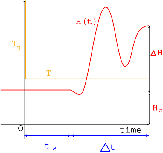
FIG. 1.: The isothermal process to consider thermodynamic properties when aging occurs. The temperature of the heat bath is decreased in a small field $H_{0}$ to a sub-critical temperature at time 0. After a waiting time $t_{w}$, the field begins to change according to a given time-dependence $H_{0}+H(t)$. This change of the field continues for a period of $\triangle t$. The waiting time $t_{w}$ and the measurement time $\triangle t$ characterize the experimental time scales.

When the field is so weak that the response is linear, the work $W$ done on the sample during the process is given in terms of the response function $R(t,t^{\prime})$ by

$$W=-\int_{t_{w}}^{t_{w}+\triangle t}dt\frac{dH(t)}{dt}M(t),$$ (1)

where the “magnetization” $M(t)$ is given by

$$M(t)=\int_{-\infty}^{0}dt^{\prime}R(t,t^{\prime})H_{0}+\int_{0}^{t}dt^{\prime}R(t,t^{\prime})H_{0}+\int_{t_{w}}^{t}dt^{\prime}R(t,t^{\prime})H(t^{\prime}).$$ (2)

Since we are interested in long waiting time behavior, the contribution of the first term of Eq. (2) is ignored. For feasibility of showing long time behavior, we rewrite Eq. (2) by integration by part to express $M(t)$ in terms of a susceptibility $\chi(t,t^{\prime})$ instead of the response function;

$$W = -H_{0}\int_{t_{w}}^{t_{w}+\triangle t}dt\frac{dH(t)}{dt}\chi(t,0)$$ (4)

$$-\int_{t_{w}}^{t_{w}+\triangle t}dt\frac{dH(t)}{dt}\int_{t_{w}}^{t}dt^{\prime}\frac{dH(t^{\prime})}{dt^{\prime}}\chi(t,t^{\prime}),$$

where the susceptibility is defined as

$$\chi(t,t^{\prime})\equiv\int_{t^{\prime}}^{t}dt^{\prime\prime}R(t,t^{\prime\prime}).$$ (5)

In order to discuss the dependence of the work on the waiting time and the measurement time, we rewrite the expression of the work by the transformations: $t\rightarrow s\equiv(t-t_{w})/\triangle t$, $H(t)\rightarrow h(s)\equiv H(s\triangle t+t_{w})/\triangle H$. We assume that $dh(s)/ds$ and $d^{2}h(s)/ds^{2}$ are finite, in order to exclude the unrealistic cases where the speed and the acceleration of changing the field is infinity. For example, the path such as $h(s)=\sqrt{s}$ is excluded, since $dh(s)/ds$ and $d^{2}h(s)/ds^{2}$ are infinite at $s=0$.

Thus, the work is reduced to

$$W/(\triangle H)^{2}=-H_{0}/\triangle H\int_{0}^{1}ds\frac{dh(s)}{ds}\chi(s\triangle t+t_{w},0)$$ (6)

$$-\int_{0}^{1}ds_{1}\frac{dh(s_{1})}{ds_{1}}\int_{0}^{s_{1}}ds_{2}\frac{dh(s_{2})}{ds_{2}}$$ (7)

$$\times\chi(s_{1}\triangle t+t_{w},s_{2}\triangle t+t_{w}),$$ (8)

which implies that the dependence of the work on the experimental time scales is determined by that of the susceptibility. Since the first term of Eq. (8) becomes a constant $-H_{0}\chi(\infty,0)/\triangle H$ in the long waiting time limit which we are interested in, we will analyze properties of the second term of Eq. (8), i.e. the work done in the zero-field cooling process ($H_{0}=0$), in the rest of this chapter for simplicity;

$$W/(\triangle H)^{2}=-\int_{0}^{1}ds_{1}\frac{dh(s_{1})}{ds_{1}}\int_{0}^{s_{1}}ds_{2}\frac{dh(s_{2})}{ds_{2}}\chi(s_{1}\triangle t+t_{w},s_{2}\triangle t+t_{w}).$$ (9)

In order to discuss behavior of the susceptibility when aging occurs, we recapitulate the long-time behavior of the response function referred to in the previous section. It is known that there are two time regimes characterized by different behavior of the correlation function $C(t,t^{\prime})$ and the FDT [6];

• At long times $t$ and $t^{\prime}$ such that $t-t^{\prime}\ll t^{\prime}$, the correlation function is the function of only the time difference $t-t^{\prime}$, i.e. the time-translational invariance (TTI) holds. In addition, although the sample is out of equilibrium, the usual FDT holds [13] as

  $$R(t-t^{\prime})=\frac{1}{k_{B}T}\frac{\partial C(t-t^{\prime})}{\partial t^{\prime}},$$ (10)

  where $C(\tau)$ is defined as $\lim_{t\rightarrow\infty}C(\tau+t,t)$. Since the properties of two-time quantities in this time regime are the same as that in equilibrium, this time regime is called the quasiequilibrium regime.

• Whereas, at long and well-separated times such that $t-t^{\prime}\sim t^{\prime}$, aging occurs, i.e. the two-time correlation function $C(t,t^{\prime})$ depends on $t^{\prime}$ even in the long time limit $t^{\prime}\rightarrow\infty$. This implies no TTI and this time regime is called the aging regime. In addition, it is known that in the aging regime the FDT is modified as

  $$R(t,t^{\prime})=\frac{X[C(t,t^{\prime})]}{k_{B}T}\frac{\partial C(t,t^{\prime})}{\partial t^{\prime}},$$ (11)

  where the FDT violation factor $X$ is a function which depends on $t,t^{\prime}$ only through the dependence of the correlation function $C(t,t^{\prime})$ [5]. Thus, a system cannot be considered to be in a quasiequilibrium state, since the usual FDT is strongly violated. When only one correlation scale exists apart from the quasiequilibrium regime, it is known that the FDT violation factor is a constant.

In order to clarify the meaning of the time region of the aging regime ($t-t^{\prime}\sim t^{\prime}$), we give an explicit expression of aging of the correlation function as

$$\lim_{{\tau\rightarrow\infty}\atop{\;\mu=t^{\prime}/g(\tau)}}C(\tau+t^{\prime},t^{\prime})=\lim_{\tau\rightarrow\infty}C[\tau+\mu g(\tau),\mu g(\tau)]\equiv\hat{C}(\mu),$$ (12)

where $g(t)$ is a system-dependent function which characterizes the aging regime and $\tau$ is the time difference $t-t^{\prime}$. The correlation function $\hat{C}(\mu)$ depends on the waiting time $t^{\prime}$ through the value of $\mu$. Occurrence of aging means that the limiting function $\hat{C}(\mu)$ takes a non-trivial value such that $0<\hat{C}(\mu)<q$. Here, $q$ is the dynamical E-A order parameter. Thus, the time region of the aging regime is the time region where $t^{\prime}/g(t-t^{\prime})$ is finite. Here, we assume that $\mu$ and $g(\tau)$ are positive.

This definition of aging is illustrated in terms of contour plot of the correlation function on $\tau-t^{\prime}$ plain (Fig. 2 (a)). The plot when aging occurs is completely different from that when aging does not occur (Fig. 2 (b)). The contour lines give the system dependent function $g(t)$ which characterizes the aging regime, since the contour lines are given by $\mu=t^{\prime}/g(\tau)$ in the contour plot.

FIG. 2.: (a) The contour plot on $\tau-t^{\prime}$ plain of the correlation function when aging occurs; $C(t,t^{\prime})=q(t^{\prime}/t)^{\gamma}\ (\gamma=0.25)$, which is the correlation function in the aging regime for the 5-spin spherical spin-glass model. The plot when aging occurs is completely different from that when aging does not occur in that the contour lines are not parallel to the horizontal axis. This contour plot gives the system-dependent function $g(t)$ which characterizes the aging regime as a contour line of the correlation function, i.e. $\mu=t^{\prime}/g(\tau)$. The straight contour lines in this figure imply that $g(\tau)$ is a linear function of $\tau$. (b) The contour plot when aging does not occur; $C(\tau+t^{\prime},t^{\prime})=\exp[-\tau/\tau_{0}]$. Since the value of the correlation function does not depend on $t^{\prime}$, the contour lines are parallel to the horizontal axis.

We show two examples of the function $g(t)$ and the aging regime for systems like spherical spin-glasses and real spin-glasses. In these systems, it is known that the correlation function behaves as a function of $\xi(t)/\xi(t^{\prime})$, where the scaling function $\xi(t)$ is a system-dependent function [2]. The function $g(t)$ is given in terms of $\xi(t)$ as $g^{-1}(t)=\xi^{-1}[r\xi(t)]-t$, where $r$ is a constant larger than unity. The inverse function of $\xi(t)$ exists since $\xi(t)$ is a monotonically increasing function. For example,

1. When $\xi(t)=t$,

   $$\lim_{{\tau\rightarrow\infty}\atop{\;\mu=t^{\prime}/\tau}}\frac{\xi(\tau+t^{\prime})}{\xi(t^{\prime})}=\lim_{{\tau\rightarrow\infty}\atop{\;\mu=t^{\prime}/\tau}}\frac{\tau+t^{\prime}}{t^{\prime}}=\lim_{\tau\rightarrow\infty}\frac{\tau+\mu\tau}{\mu\tau}=\frac{1+\mu}{\mu}.$$ (13)

   Thus, $\lim_{{\tau\rightarrow\infty}\atop{\;\mu=t^{\prime}/\tau}}C(\tau+t^{\prime},t^{\prime})$ is a function of $\mu$ and hence the aging regime is the time regime where $t^{\prime}/\tau$ is finite.

2. When $\xi(t)=\exp[(t/\tau_{0})^{1-\alpha}/(1-\alpha)](0<\alpha<1)$,

   $$\lim_{{\tau\rightarrow\infty}\atop{\;\mu=t^{\prime}/\tau^{1/\alpha}}}\frac{\xi(\tau+t^{\prime})}{\xi(t^{\prime})}=\exp(\tau_{0}^{\alpha-1}\mu^{-\alpha}).$$ (14)

   Thus, $\lim_{{\tau\rightarrow\infty}\atop{\;\mu=t^{\prime}/\tau^{1/\alpha}}}C(\tau+t^{\prime},t^{\prime})$ is a function of $\mu$ and hence the aging regime is the time regime when $t^{\prime}/\tau^{1/\alpha}$ is finite.

From these results, it is shown by the definition of the susceptibility Eq. (5) that the behavior of the susceptibility depends on the time regimes according to the dependence of the behavior of the response function. In the quasiequilibrium regime, the susceptibility depends only on the time difference $\tau\equiv t-t^{\prime}$ and is given by the correlation function as

$$\chi(\tau)=-\frac{1}{k_{B}T}[C(\tau)-C(0)]$$ (15)

where $C(\tau)\equiv\lim_{t^{\prime}\rightarrow\infty}C(\tau+t^{\prime},t^{\prime})$. Whereas, in the aging regime, time translational invariance (TTI) does not hold and the susceptibility is given by the correlation function as

$$\chi(t,t^{\prime})=\frac{1}{k_{B}T}\int_{C(t,t^{\prime})}^{C(t,t)}dCX(C)$$ (16)

where $X$ is the FDT violation factor defined by Eq. (11). It implies that the susceptibility is a function of the correlation function.

Since the difference of the two arguments of the susceptibility in Eq. (9) is $(s_{1}-s_{2})\triangle t$, there are also two time regimes characterized by different dependence of the work on the experimental time scales $\triangle t$ and $t_{w}$.

• When the waiting time is much longer than the measurement time ($\triangle t\ll t_{w}$), the susceptibility which appears in Eq. (9) obeys Eq. (15) since $(s_{1}-s_{2})\triangle t\ll s_{2}\triangle t+t_{w}$ holds. Hence, from Eqs. (9) and (15) the work in this regime is written as

  $$W/(\triangle H)^{2} = -\frac{C(0)}{2k_{B}T}+\frac{1}{k_{B}T}\int_{0}^{1}ds_{1}\frac{dh(s_{1})}{ds_{1}}$$ (18)

  $$\times\int_{0}^{s_{1}}ds_{2}\frac{dh(s_{2})}{ds_{2}}C[(s_{1}-s_{2})\triangle t].$$

  In the derivation,

  $$\int_{0}^{1}ds_{1}\frac{dh(s_{1})}{ds_{1}}\int_{0}^{s_{1}}ds_{2}\frac{dh(s_{2})}{ds_{2}}=1/2$$ (19)

  for any path $h(s)$ is used.

• On the other hand, when both the waiting time and the measurement time are long ($\triangle t\sim t_{w}$), the susceptibility obeys Eq. (16) since $(s_{1}-s_{2})\triangle t\sim s_{2}\triangle t+t_{w}$ holds [15]. In this regime, it is seen from Eq. (16) that the work is a functional of the correlation function which shows aging. The ambiguous relation $t_{w}\sim\triangle t$ is described explicitly in Sec. IV with the function $g(t)$ defined in Eq. (12).

We refer to the former case as the quasiequilibrium regime and the latter case as the aging regime without any confusion with the time regimes characterized by the behavior of the correlation and the response function.

III the work in the quasiequilibrium regime

In this section, we investigate the properties of the work done on the sample when the measurement time $\triangle t$ is short compared to the long waiting time $t_{w}$ (the quasiequilibrium regime).

A The work done in an slow process

First, we derive the work done in an slow operation such that the measurement time $\triangle t$ is so long that the correlation function relax to a time-independent value. This process is formulated by taking the infinite measurement time limit $\triangle t\rightarrow\infty$. Glassy systems are out of equilibrium even in such an infinitely slow process. Hence, we call a process where the external field is changed infinitely slowly a “slow process” instead of a “quasistatic process”.

Since for the slow process the time lapse of the process is infinity, the work done in the slow process in the quasiequilibrium regime is given by taking the limit $\triangle t\rightarrow\infty$ after taking the infinite waiting time limit of Eq. (18). Since the integrand, the correlation function, is finite, the order of limit and integration can be changed. Thus, we can write the work $W_{s}$ for the slow process as

$$W_{s}/(\triangle H)^{2} = \lim_{\triangle t\rightarrow\infty}\lim_{t_{w}\rightarrow\infty}W/(\triangle H)^{2}$$ (20)

$$= -\frac{C(0)}{2k_{B}T}+\frac{1}{k_{B}T}\ \int_{0}^{1}ds_{1}\frac{dh(s_{1})}{ds_{1}}$$ (22)

$$\times\int_{0}^{s_{1}}ds_{2}\frac{dh(s_{2})}{ds_{2}}\lim_{\triangle t\rightarrow\infty}C[(s_{1}-s_{2})\triangle t].$$

Here, in order to give the expression of the work $W_{s}$, we introduce the dynamical Edwards-Anderson (E-A) order parameter defined as

$$q\equiv\lim_{\tau\rightarrow\infty}\lim_{t_{w}\rightarrow\infty}C(\tau+t_{w},t_{w}).$$ (23)

Using Eq. (19) and the above definition, the work $W_{s}$ for the slow process is given by

$$W_{s}=-\frac{(\triangle H)^{2}}{2k_{B}T}[C(0)-q].$$ (24)

Therefore, the work for the slow process in the quasiequilibrium regime is the difference of a state function, since the right hand side of Eq. (24) is independent of the path of changing the field $h(s)$ and dependent only on the thermodynamic variables ($\triangle H$ and $T$) and constants intrinsic to the system ($C(0)$ and $q$). It is important to note that this property is derived by using only the FDT.

On the other hand, for usual systems apart from glassy systems, one may expect that equilibrium is usually achieved when $t_{w}$ is long ($t_{w}\rightarrow\infty$). So, thermodynamics can be applied and the work for the slow process is equal to the change of the Helmholtz free energy, $\triangle F_{eq}$, calculated by equilibrium statistical mechanics. However, we show below that this naive expectation fails for glassy systems. More precisely, the work for the slow process, Eq. (24), is different from the change of the Helmholtz free energy calculated by equilibrium statistical mechanics. It is because the glassy systems are out of equilibrium even when the waiting time is infinite.

Assuming that $A(t)$ is a physical quantity coupled to the external field $H(t)$ linearly, we see from statistical mechanics with the assumption of ergodicity that the isothermal susceptibility $\chi_{T}$ is given by

$$\chi_{T}=\frac{1}{k_{B}T}\langle\langle A^{2}\rangle_{eq}-\langle A\rangle^{2}_{eq}\rangle_{J}$$ (25)

where $\langle\cdots\rangle_{eq}$ denotes average over the Gibbs-Boltzmann distribution and $\langle\cdots\rangle_{J}$ denotes disorder-average. Thus, the free energy difference $\triangle F_{eq}$ due to change $\triangle H$ of the external field is

$$\triangle F_{eq}=-\frac{(\triangle H)^{2}}{2k_{B}T}\langle\langle A^{2}\rangle_{eq}-\langle A\rangle^{2}_{eq}\rangle_{J}$$ (26)

where $\langle\langle A\rangle^{2}_{eq}\rangle_{J}$ is the usual E-A order parameter. Since ergodicity is broken for glassy systems, the phase space decomposes into many pure states. Assuming that $\langle\cdots\rangle_{a}$ denotes the thermal average in local equilibrium in the pure state $a$ and $F_{a}$ denotes the free energy at the pure state $a$, we see that

$$\langle A^{2}\rangle_{eq}=\sum_{a}P^{eq}_{a}\langle A^{2}\rangle_{a},$$ (27)

$$\langle A\rangle_{eq}^{2}=(\sum_{a}P^{eq}_{a}\langle A\rangle_{a})^{2}.$$ (28)

where $P_{a}^{eq}$ is the probability that the system is found at the pure state $a$ in true equilibrium and is given by $P_{a}^{eq}\equiv\exp(-\beta F_{a})/Z$.

In order to compare $W_{s}$, Eq. (24), with $\triangle F_{eq}$, Eq. (26), we rewrite Eq. (24) in terms of pure states. Since the correlation function is given by $C(t,t^{\prime})=\langle\langle A(t)A(t^{\prime})\rangle\rangle_{J}$ and the local equilibrium in pure states is achieved in the long time limit,

$$C(0)\equiv\lim_{t^{\prime}\rightarrow\infty}\langle\langle{A(t^{\prime})}^{2}\rangle\rangle_{J}=\sum_{a}P^{ini}_{a}\langle\langle A^{2}\rangle_{a}\rangle_{J},$$ (29)

$$q\equiv\lim_{\tau\rightarrow\infty}\lim_{t^{\prime}\rightarrow\infty}\langle\langle A(\tau+t^{\prime})A(t^{\prime})\rangle\rangle_{J}=\sum_{a}P^{ini}_{a}\langle\langle A\rangle_{a}^{2}\rangle_{J}$$ (30)

where $P^{ini}_{a}$ is the probability that the system is found in pure state $a$ at time $0$. Since the system is out of equilibrium at time $0$, $P_{a}^{eq}\neq P_{a}^{ini}$. Thus, $\langle\langle A^{2}\rangle_{eq}\rangle_{J}$ is not equal to $C(0)$. In addition, from Eqs. (28) and (30), $\langle\langle A\rangle_{eq}^{2}\rangle_{J}$ is not equal to $q$. Consequently, we conclude that the work $W_{s}$ for the slow process does not coincide with the free energy difference calculated by statistical mechanics with assumption of ergodicity.

B The work when the measurement time is finite

We discuss the properties of the work when the measurement time is finite. From Eqs. (18) and (24), the difference between the work when the process is not slow and the work for the slow process is given by

$$W-W_{s}=\frac{(\triangle H)^{2}}{k_{B}T}\int_{0}^{1}ds_{1}\frac{dh(s_{1})}{ds_{1}}\int_{0}^{s_{1}}ds_{2}\frac{dh(s_{2})}{ds_{2}}\{C[(s_{1}-s_{2})\triangle t]-q\}.$$ (31)

$C[(s_{1}-s_{2})\triangle t]>q$ when $\triangle t$ is finite, since the quasiequilibrium regime is considered. Hence, the difference from the work for the slow process is positive for any path of changing the field, when the measurement time is finite. This implies the principle of minimum work;

$$W\geq W_{s},$$ (32)

where the equality holds only when the measurement time is infinite, i.e. the slow-process limit.

Our result is very similar to the consequence of thermodynamics which tells the work for non-quasistatic process is larger than the change of the Helmholtz free energy. However, our result is different from that and beyond the scope of thermodynamics since in our discussion the initial state and the final state of the process are out of equilibrium and the value of the work for the slow process is different from the value of change in the Helmholtz free energy derived by equilibrium statistical mechanics.

C Long measurement time behavior of $W-W_{s}$

The long measurement time behavior of $W-W_{s}$ is analyzed in this subsection. We show that the behavior of $W-W_{s}$ when the measurement time $\triangle t$ is long but finite is determined by the long time behavior of the correlation function. We describe below the results for four types of behavior of the correlation function which include almost all types of relaxation of the correlation, e.g., the exponential, the power law [16], the logarithmic [17] and the stretched exponential relaxation [18]. The derivations are given in Appendix A.

1. When the correlation function behaves as $\lim_{\tau\rightarrow\infty}\tau[C(\tau)-q]=0$, the difference is given by

   $$W-W_{s}\simeq\frac{(\triangle H)^{2}}{k_{B}T}K_{\infty}\int_{0}^{1}ds\left|\frac{dh(s)}{ds}\right|^{2}\frac{1}{\triangle t},$$ (33)

   where

   $$K_{\infty}\equiv\int_{0}^{\infty}d\tau[C(\tau)-q]$$ (34)

   and $W_{s}$ denotes the work for the slow process. This case includes the power law relaxation such that $C(\tau)\simeq q+c\tau^{-\alpha}$ when $\alpha>1$ and the stretched exponential relaxation ($\exp(-a\tau^{n}),0<n<1$) as well as the exponential relaxation [19].

2. When the correlation function behaves as $\lim_{\tau\rightarrow\infty}\tau[C(\tau)-q]=c$, the difference is given by

   $$W-W_{s}\simeq\frac{(\triangle H)^{2}}{k_{B}T}c\int_{0}^{1}ds\left|\frac{dh(s)}{ds}\right|^{2}\frac{\ln(\triangle t)}{\triangle t}.$$ (35)

   These two results show that $W-W_{s}$ is proportional to the inverse of the measurement time only when $\lim_{\tau\rightarrow\infty}\tau[C(\tau)-q]=0$. In these two cases, the difference from the work for the slow process takes the minimum value when the field increases linearly as $h(s)=s$, since we assume that $dh(s)/ds$ and $d^{2}h(s)/ds^{2}$ is finite.

3. When the correlation function obeys the power law relaxation, such that $C(\tau)\simeq q+c\tau^{-\alpha}$ ($0<\alpha<1$), the difference is given by

   $$W-W_{s} \simeq \frac{(\triangle H)^{2}}{k_{B}T}c\int_{0}^{1}ds_{1}\frac{dh(s_{1})}{ds_{1}}$$ (37)

   $$\times\int_{0}^{s_{1}}ds_{2}\frac{dh(s_{2})}{ds_{2}}\frac{1}{(s_{1}-s_{2})^{\alpha}}\frac{1}{(\triangle t)^{\alpha}}.$$

   In this case, the difference from $W_{s}$ obeys the power law whose exponent is equal to the exponent of the correlation function.

4. When the correlation function obeys the logarithmic relaxation $C(\tau)\simeq q+c/\ln(\tau)$, the difference also obeys the logarithmic relaxation as

   $$W-W_{qs}=\frac{(\triangle H)^{2}}{2k_{B}T}\frac{c}{\ln(\triangle t)}+O[\frac{\ln(\ln\triangle t)}{(\ln\triangle t)^{2}}].$$ (38)

   In this case, the difference does not depend on the path $h(s)$.

Experimentally, these results tell how long the measurement should take and the suitable path of changing the external field in order to determine the value of the work for the slow process, i.e. the difference of a state function in quasiequilibrium regime.

IV The work in the aging regime; general results

In this section, we discuss the properties of the work in the isothermal slow process when both the waiting time and the measurement time are long, i.e. in the aging regime, by using the modified FDT and aging of the correlation function introduced in Eqs. (11) and (12). Condition when the work for the slow process depends on the path changing the external field is obtained. By using the results obtained in this section, the path-dependence of the work for particular systems is discussed in the next section, Sec. V.

A Path-dependence of the work for the slow process

As shown in Sec. II, in the aging regime the work is a functional of the correlation function which shows aging. The slow process of the aging regime is given by taking the long measurement time limit $\triangle t\rightarrow\infty$ with holding the relation $t_{w}\sim\triangle t$, which guarantees that the slow-process limit is taken within the aging regime. The slow-process limit has always this meaning in this section.

The order of the slow-process limit and the integration can be changed since the susceptibility $\chi$ is finite. From Eq. (9) the work $W_{s}$ for the slow process in the aging regime is given by

$$W_{s}/(\triangle H)^{2} = -\int_{0}^{1}ds_{1}\frac{dh(s_{1})}{ds_{1}}\int_{0}^{s_{1}}ds_{2}\frac{dh(s_{2})}{ds_{2}}$$ (40)

$$\times\chi[\lim_{{\triangle t\rightarrow\infty}\atop{\;t_{w}\sim\triangle t}}C(s_{1}\triangle t+t_{w},s_{2}\triangle t+t_{w})].$$

Thus, the dependence of $\lim_{{\triangle t\rightarrow\infty}\atop{\;t_{w}\sim\triangle t}}C(s_{1}\triangle t+t_{w},s_{2}\triangle t+t_{w})$ on $s_{1}$ and $s_{2}$ determines the dependence of the work for the slow process on the path of changing the field $h(s)$; $W_{s}$ is independent of $h(s)$ if $\lim_{{\triangle t\rightarrow\infty}\atop{\;t_{w}\sim\triangle t}}C(s_{1}\triangle t+t_{w},s_{2}\triangle t+t_{w})$ does not depend on $s_{1}$ and $s_{2}$. On the other hand, $W_{s}$ is a functional of $h(s)$ if $\lim_{{\triangle t\rightarrow\infty}\atop{\;t_{w}\sim\triangle t}}C(s_{1}\triangle t+t_{w},s_{2}\triangle t+t_{w})$ depends on $s_{1}$ and $s_{2}$. We derive conditions when $W_{s}$ depends on $h(s)$ in the rest of this section.

In order to analyze $\lim_{{\triangle t\rightarrow\infty}\atop{\;t_{w}\sim\triangle t}}C(s_{1}\triangle t+t_{w},s_{2}\triangle t+t_{w})$, we clarify the meaning of $t_{w}\sim\triangle t$ or the aging regime by using $g(\tau)$ in Eq. (12). By substitution $t^{\prime}\rightarrow s_{2}\triangle t+t_{w},\tau\rightarrow(s_{1}-s_{2})\triangle t$ in Eq. (12), we see that the following equation holds in the region except for the point $s_{1}=s_{2}$ which does not contribute to the value of the work by itself;

$$\lim_{{\triangle t\rightarrow\infty}\atop{\;\mu=\frac{s_{2}\triangle t+t_{w}}{g[(s_{1}-s_{2})\triangle t]}}}C(s_{1}\triangle t+t_{w},s_{2}\triangle t+t_{w})=\hat{C}(\mu).$$ (41)

This equation implies that the aging regime is the experimental time regime where $(s_{2}\triangle t+t_{w})/g[(s_{1}-s_{2})\triangle t]$ is finite and the slow-process limit of the correlation function in the integrand in Eq. (40) is a function of $\lim_{{\triangle t\rightarrow\infty}\atop{\;t_{w}\sim\triangle t}}(s_{2}\triangle t+t_{w})/g[(s_{1}-s_{2})\triangle t]$.

We discuss below the aging regimes and dependence of $\lim_{{\triangle t\rightarrow\infty}\atop{\;t_{w}\sim\triangle t}}C(s_{1}\triangle t+t_{w},s_{2}\triangle t+t_{w})$ on $s_{1}$ and $s_{2}$ in four cases of the different long-time behaviors of $g(t)$ which exhaust all possibilities (see Fig. 3).

FIG. 3.: The schematic illustration of the four types of the long-time behavior of the function $g(\tau)$. For example, $g(\tau)=\log\tau$ (type 1.), $g(\tau)=\tau$ (type 2.), $g(\tau)={\tau}^{2}$ (type 3.), $g(\tau)=\exp{\tau}$ (type 4.) are plotted against $1/\tau$. It is important to note that these four types exhaust all possibilities of long-time behavior.

1. When $\lim_{\tau\rightarrow\infty}\tau/g(\tau)=\infty$, $t^{\prime}/g(t-t^{\prime})$ is finite only in the region $t^{\prime}\ll t-t^{\prime}$. In the region of integration of Eq. (40) except for the point $s_{2}=0$,

   $$(s_{2}\triangle t+t_{w})/g[(s_{1}-s_{2})\triangle t]\rightarrow\infty$$ (42)

   as $\triangle t\rightarrow\infty$ since $t_{w}>0$. An example of such $g(\tau)$ is $g(\tau)=\log\tau$. When $g(\tau)=\log\tau$ and $s_{2}\neq 0$, $\lim_{\triangle t\rightarrow\infty}(s_{2}\triangle t+t_{w})/g[(s_{1}-s_{2})\triangle t]=\infty$ as shown in Eq. (42). Since the point $s_{2}=0$ does not contribute to the value of the work by itself, the experimental time regime where $(s_{2}\triangle t+t_{w})/g[(s_{1}-s_{2})\triangle t]$ is finite does not exist in this case. If there is no other aging regime except for that characterized by such $g(\tau)$ exists, only the quasiequilibrium regime contributes to the value of the work and hence the work for the slow process is independent of $h(s)$ and is given by Eq. (24).

2. When $g(\tau)=\tau$,

   $$\frac{s_{2}\triangle t+t_{w}}{g[(s_{1}-s_{2})\triangle t]}=\frac{s_{2}\triangle t+t_{w}}{(s_{1}-s_{2})\triangle t}=\frac{s_{2}+t_{w}/\triangle t}{s_{1}-s_{2}}.$$ (43)

   Thus, from Eq. (41), $\lim_{{\triangle t\rightarrow\infty}\atop{\;\mu^{\prime}=t_{w}/\triangle t}}C(s_{1}\triangle t+t_{w},s_{2}\triangle t+t_{w})$ is a function of $(s_{2}+\mu^{\prime})/(s_{1}-s_{2})$;

   $$\lim_{{\triangle t\rightarrow\infty}\atop{\;\mu^{\prime}=t_{w}/\triangle t}}C(s_{1}\triangle t+t_{w},s_{2}\triangle t+t_{w})$$ (44)

   $$= \lim_{{\triangle t\rightarrow\infty}\atop{\;\frac{s_{2}+\mu^{\prime}}{s_{1}-s_{2}}=\frac{s_{2}\triangle t+t_{w}}{g[(s_{1}-s_{2})\triangle t]}}}C(s_{1}\triangle t+t_{w},s_{2}\triangle t+t_{w})$$ (45)

   $$= \hat{C}(\frac{s_{2}+\mu^{\prime}}{s_{1}-s_{2}}).$$ (46)

   It implies that the aging regime is the region where $t_{w}/\triangle t$ is finite. In this aging regime the slow-process limit of the correlation function in the integrand of Eq. (40) depends on $s_{1}$ and $s_{2}$ if $f(\mu)$ in Eq. (41) is not a constant. It means that the work for the slow process, $W_{s}$, depends on the path of change of the external field, $h(s)$.

3. When $\lim_{\tau\rightarrow\infty}\tau/g(\tau)=0$ and $\lim_{\tau\rightarrow\infty}g(\tau)/g(s\tau)\equiv g_{r}(s)\ (s<1)$ exists,

   $$\frac{s_{2}\triangle t+t_{w}}{g[(s_{1}-s_{2})\triangle t]}=\frac{s_{2}\triangle t+t_{w}}{g(\triangle t)}\frac{g(\triangle t)}{g[(s_{1}-s_{2})\triangle t]}$$ (47)

   $$\rightarrow\frac{t_{w}}{g(\triangle t)}g_{r}(s_{1}-s_{2}),$$ (48)

   as $\triangle t\rightarrow\infty$. An example of such $g(\tau)$ is $g(\tau)={\tau}^{\alpha}\ (\alpha>1)$. When $g(\tau)={\tau}^{\alpha}\ (\alpha>1)$, Eq. (48) holds;

   $$\frac{s_{2}\triangle t+t_{w}}{g[(s_{1}-s_{2})\triangle t]}\rightarrow\frac{t_{w}}{g(\triangle t)}\frac{1}{(s_{1}-s_{2})^{\alpha}}$$ (49)

   as $\triangle t\rightarrow\infty$. From Eqs. (41) and (48),

   $$\lim_{{\triangle t\rightarrow\infty}\atop{\;\mu^{\prime}=t_{w}/g(\triangle t)}}C(s_{1}\triangle t+t_{w},s_{2}\triangle t+t_{w})$$ (50)

   $$= \lim_{{\triangle t\rightarrow\infty}\atop{\;\mu^{\prime}g_{r}(s_{1}-s_{2})=\frac{s_{2}\triangle t+t_{w}}{g[(s_{1}-s_{2})\triangle t]}}}C(s_{1}\triangle t+t_{w},s_{2}\triangle t+t_{w})$$ (51)

   $$= \hat{C}[\mu^{\prime}g_{r}(s_{1}-s_{2})].$$ (52)

   It implies that the aging regime is the region where $t_{w}/g(\triangle t)$ is finite. In this aging regime the slow-process limit of the correlation function in the integrand of Eq. (40) is a function of $s_{1}$ and $s_{2}$ if $f(\mu)$ in Eq. (41) is not a constant. It means that the work $W_{s}$ depends on $h(s)$.

4. When $\lim_{\tau\rightarrow\infty}\tau/g(\tau)=0$ and $\lim_{\tau\rightarrow\infty}g(\tau)/g(s\tau)=\infty\ (s<1)$, we prove below that the aging regime for experimental time scales does not exist. We assume that the aging regime exists. It means that a function $p(t)$ exists such that $\lim_{{\triangle t\rightarrow\infty}\atop{\;\mu=t_{w}/p(\triangle t)}}(s_{2}\triangle t+t_{w})/g[(s_{1}-s_{2})\triangle t]$ is finite. Then, from the condition $\lim_{\tau\rightarrow\infty}\tau/g(\tau)=0$,

   $$\lim_{{\triangle t\rightarrow\infty}\atop{\;\mu=\frac{t_{w}}{p(\triangle t)}}}\frac{s_{2}\triangle t+t_{w}}{g[(s_{1}-s_{2})\triangle t]}$$ (53)

   $$= \lim_{{\triangle t\rightarrow\infty}\atop{\;\mu=\frac{t_{w}}{p(\triangle t)}}}\frac{t_{w}}{g[(s_{1}-s_{2})\triangle t]}$$ (54)

   $$= \lim_{\triangle t\rightarrow\infty}\frac{\mu p(\triangle t)}{g[(s_{1}-s_{2})\triangle t]}.$$ (55)

   Assuming that $s^{\prime}_{1}-s^{\prime}_{2}>s_{1}-s_{2}$, we see from the condition $\lim_{\tau\rightarrow\infty}g(\tau)/g(s\tau)=\infty\ (s<1)$ that

   $$\lim_{{\triangle t\rightarrow\infty}\atop{\;\mu=\frac{t_{w}}{p(\triangle t)}}}\frac{s_{2}\triangle t+t_{w}}{g[(s_{1}-s_{2})\triangle t]}/\lim_{{\triangle t\rightarrow\infty}\atop{\;\mu=\frac{t_{w}}{p(\triangle t)}}}\frac{s^{\prime}_{2}\triangle t+t_{w}}{g[(s^{\prime}_{1}-s^{\prime}_{2})\triangle t]}$$ (56)

   $$= \lim_{\triangle t\rightarrow\infty}\frac{\mu p(\triangle t)}{g[(s_{1}-s_{2})\triangle t]}\frac{g[(s^{\prime}_{1}-s^{\prime}_{2})\triangle t]}{\mu p(\triangle t)}$$ (57)

   $$= \lim_{\triangle t\rightarrow\infty}\frac{g[(s^{\prime}_{1}-s^{\prime}_{2})\triangle t]}{g[(s_{1}-s_{2})\triangle t]}$$ (58)

   $$= \infty.$$ (59)

   Since Eq. (59) contradicts the assumption that $\lim_{{\triangle t\rightarrow\infty}\atop{\;\mu=t_{w}/p(\triangle t)}}(s_{2}\triangle t+t_{w})/g[(s_{1}-s_{2})\triangle t]$ is finite, the aging regime for experimental time scales does not exist in this case. Hence, if only this aging regime characterized by such $g(t)$ exists, $\lim_{{\triangle t\rightarrow\infty}\atop{\;t_{w}\sim\triangle t}}C(s_{1}\triangle t+t_{w},s_{2}\triangle t+t_{w})$ is equal to $0$ or $q$. It implies that the work is independent of $h(s)$. An example of such $g(t)$ is $g(t)=\exp(t)$.

Consequently, we conclude that if there are aging regimes characterized by $g(\tau)$ of case 2. or case 3. and the function $\hat{C}(\mu)$ is not a constant and the FDT violation factor $X$ is not equal to $0$, the work for the slow process depends on the path of changing the external field $h(s)$. In this case, contrary to the fundamental assumption of thermodynamics, the work for the slow process is not the difference of a state function.

V The work in the aging regime; results for single-correlation-scale systems and multi-correlation-scale systems

It has been explicitly checked on several disordered models that in the long-time limit two situations with different dynamical behavior seem to exist [2]:

• There are systems with only one correlation scale apart from the quasiequilibrium regime, which we call “single-correlation-scale systems”. For these systems, the correlation function scales as $C(t,t^{\prime})=C[\xi(t)/\xi(t^{\prime})]$ and the FDT violation factor $X$ is a constant. Equilibrium states of these systems are solved by a one step replica symmetry breaking ansatz. Examples are the $p$-spin spherical spin-glasses [4] and a Lennard-Jones binary mixture which is a model of structural glasses in a glassy state [10]. The real spin-glasses such as AgMn seem to belong to this class since it is known that the correlation function is scaled with single scaling function $\xi(t)$.

• There are systems such as Sherrington-Kirkpatrick (S-K) model which have an infinite number of correlation-scales apart from the quasiequilibrium regime [5], which we call “multi-correlation-scale systems”. For these systems, ultrametricity in time holds for any correlation such that $C(t,t^{\prime})<q$; $C(t_{1},t_{3})=\min[C(t_{1},t_{2}),C(t_{2},t_{3})]\ \mbox{when}\ t_{1}>t_{2}>t_{3}\ \mbox{and}\ t_{3}\rightarrow\infty$. The FDT violation factor $X$ is a nontrivial function of $C$. Equilibrium properties of these systems are solved by a full replica-symmetry breaking ansatz.

In this section, we analyze the path-dependence of the work for the slow process in the aging regime for these two classes of systems by using the general results obtained in the previous section, Sec. IV. It is important to note that only these two classes of systems seem to exist [2].

A The single-correlation-scale systems

For the single-correlation-scale systems, scaling of the correlation function $C(t,t^{\prime})=C[\xi(t)/\xi(t^{\prime})]$ holds. Hence, the work for the slow process in the aging regime is given as

$$W_{s}/(\triangle H)^{2} = -\int_{0}^{1}ds_{1}\dot{h}(s_{1})\int_{0}^{s_{1}}ds_{2}\dot{h}(s_{2})$$ (61)

$$\times\chi\{C[\lim_{{\triangle t\rightarrow\infty}\atop{\;t_{w}\sim\triangle t}}\frac{\xi(s_{1}\triangle t+t_{w})}{\xi(s_{2}\triangle t+t_{w})}]\}.$$

Three explicit choices of the scaling function $\xi(t)$ have been proposed so far; $\xi(t)=t,\xi(t)=\exp[(t/\tau_{0})^{1-\alpha}/(1-\alpha)]$ and $\xi(t)=\exp[\ln^{a}(t/\tau_{0})]$ [2]. We analyze below the properties of the work for the slow process for each three cases.

1. When $\xi(t)=t$, the correlation function decays in power-law as found in the trap model [21] and the $p$-spin spherical spin-glasses [4]. The slow-process limit of the correlation function in Eq. (61) depends on $s_{1}$ and $s_{2}$ as

   $$\lim_{{\triangle t\rightarrow\infty}\atop{\;\mu=\frac{t_{w}}{\triangle t}}}\frac{\xi(s_{1}\triangle t+t_{w})}{\xi(s_{2}\triangle t+t_{w})}=\frac{s_{1}+\mu}{s_{2}+\mu}.$$ (62)

   This is an example of Eq. (46) in previous section.

2. When $\xi(t)=\exp[\frac{1}{1-\alpha}(\frac{t}{\tau_{0}})^{1-\alpha}](\alpha<1)$ [22], the slow-process limit of the correlation function in Eq. (61) depends on $s_{1}$ and $s_{2}$ through the scaling function which behaves as

   $$\lim_{{\triangle t\rightarrow\infty}\atop{\;\mu=t_{w}/\triangle t^{1/\alpha}}}\frac{\xi(s_{1}\triangle t+t_{w})}{\xi(s_{2}\triangle t+t_{w})}=\exp[\frac{\mu}{\tau_{0}^{1-\alpha}}(s_{1}-s_{2})].$$ (63)

   This is an example of Eq. (52).

3. When $\xi(t)=\exp[\ln^{a}(t/\tau_{0})](a>1)$ [26], the slow-process limit of the correlation function which appears in Eq. (61) depends on $s_{1}$ and $s_{2}$ through the scaling function which behaves as

   $$\lim_{{\triangle t\rightarrow\infty}\atop{\;\mu=\triangle t/(t_{w}\ln^{1-a}t_{w})}}\frac{\xi(s_{1}\triangle t+t_{w})}{\xi(s_{2}\triangle t+t_{w})}=\exp[a\mu(s_{1}-s_{2})].$$ (64)

   This is another example of Eq. (52)

To my knowledge, only three types of the scaling function $\xi(t)$ discussed above are known so far for single-correlation-scale systems. For each of three cases the slow-process limit of the correlation function in the integrand of Eq. (40) is a function of $s_{1}$ and $s_{2}$. It means for the single-correlation-scale systems that the work for the slow process in the aging regime depends on the path of changing the external field $h(s)$ and contrary to the assumption of thermodynamics the work for the slow process is not a difference of a state function.

In order to see more explicit form of the work for the slow process in the aging regime, we introduce the modified FDT Eq. (11) with constant violation factor $X$ which has been verified to be valid for the single-correlation-scale systems [5].

From Eq. (11), the susceptibility is given by

$$\chi(t,t^{\prime})=-\frac{1}{k_{B}T^{eff}}C(t,t^{\prime})+\frac{q}{k_{B}T^{eff}}-\frac{C(0)-q}{k_{B}T},$$ (65)

where $C(0)\equiv\lim_{t^{\prime}\rightarrow\infty}C(t^{\prime},t^{\prime})$. Hence, from Eq. (40), the work for the slow process is given by

$$W_{s}/(\triangle H)^{2}=-\frac{C(0)-q}{2k_{B}T}-\frac{1}{k_{B}T^{eff}}\int_{0}^{1}ds_{1}\frac{dh(s_{1})}{ds_{1}}\int_{0}^{s_{1}}ds_{2}\frac{dh(s_{2})}{ds_{2}}$$ (66)

$$\times\{q-\lim_{{\triangle t\rightarrow\infty}\atop{\;t_{w}\sim\triangle t}}C[\xi(s_{1}\triangle t+t_{w})/\xi(s_{2}\triangle t+t_{w})]\}.$$ (67)

Since $\lim_{{\triangle t\rightarrow\infty}\atop{\;t_{w}\sim\triangle t}}C(s_{1}\triangle t+t_{w},s_{2}\triangle t+t_{w})<q$ when $s_{1}\neq s_{2}$, the second term on the right hand side is non-zero. Hence, if $T^{eff}$ is finite the work for the slow process is not the difference of a state function since the work depends on the path of changing the field $h(s)$. In addition, the value of the work is different from the value of the work for the slow process in the quasiequilibrium regime: the first term on the right hand side of Eq. (67). In addition, it is also shown that since the correlation function is positive and smaller than the dynamical E-A order parameter in this regime, there are bounds for the value of the quasistatic work as

$$-\frac{C(0)-q}{2k_{B}T}-\frac{q}{2k_{B}T^{eff}}\leq\frac{W_{s}}{(\triangle H)^{2}}\leq-\frac{C(0)-q}{2k_{B}T}.$$ (68)

Eq. (68) shows that the work $W_{s}$ in the aging regime is independent of the path of changing the field and coincides with the work $W_{s}$ in the quasiequilibrium regime when the effective temperature $T^{eff}$ is infinite, which holds for the $2$-spin spherical spin-glass model [28] and a model of phase separation [12].

B Possibility of observation of path-dependence

In the previous subsection, we saw that the work for the slow process depends on the path of changing the external field when $\triangle t\sim t_{w}$. We show here that the path-dependence of the work for the slow process is strong enough to be observed in experiments by evaluating the path-dependence of the $5$-spin spherical spin-glass model.

First, we describe the several pieces of information needed to evaluate Eq. (67). It is known that the scaling of the correlation function, such that $C(t,t^{\prime})\simeq q(t^{\prime}/t)^{\gamma}$ and the modified FDT with the effective temperature, i.e. Eq. (11), hold for the model [4]. When $k_{B}T/J=0.2$ [29], $\gamma\simeq 0.25$ has been obtained. The dynamical E-A parameter $q$ and the effective temperature are given by $q\simeq 0.929$ and $T/T^{eff}\simeq 0.227$ when $k_{B}T/J=0.2$. In computation of these values, we uses the formulae:

$\displaystyle q^{3}(1-q)^{2}=\frac{(k_{B}T)^{2}}{10},\ \ \frac{T}{T^{eff}}=\frac{3(1-q)}{q}.$

In order to evaluate the magnitude of the path-dependence, we compute the relative difference between the works for two paths ($h(s)=s$ and $h(s)=s^{2}$) which is defined as the difference between the works for the two paths divided by the average of the two works. The results obtained from Eq. (67) are as follows; When the ratio of the measurement time to the waiting time is $1:1$, the relative difference is equal to $0.037$, i.e. about $4\%$; When the ratio is $5:1$, the relative difference is equal to $0.094$, i.e. about $9\%$.

Hence, we can say that the path-dependence of the work in the slow process can be observed for the $5$-spin spherical spin-glass model. The relative difference is plotted against the ratio of the waiting time to the measurement time in Fig. 4.

FIG. 4.: The relative difference between the works for the two paths ($h(s)=s$ and $h(s)=s^{2}$) of changing the field infinitely slowly is plotted against the ratio of the waiting time to the measurement time for the $5$-spin spherical spin-glass model. The path-dependence of the work for the slow process in the aging regime is strong enough to be observed in simulations for the model. In addition, we see that the path-dependence becomes larger, as one increases the measurement time with keeping the waiting time fixed.

It tells that contrary to intuition the path-dependence becomes larger, as one increases the measurement time with keeping the waiting time fixed.

C The multi-correlation-scale systems

For the multi-correlation-scale systems such as S-K model, it is known that the ultrametricity in time holds for all correlations such that $C(t,t^{\prime})<q$ in the long-time limit [5];

$$C(t_{1},t_{3})=\min[C(t_{1},t_{2}),C(t_{2},t_{3})]\ \ \mbox{when}\ t_{1}>t_{2}>t_{3}.$$ (69)

By using this ultrametric relation Eq. (69), we prove below that the correlation function in the aging regime is a constant in the two cases (case 2 and case 3 in Sec. IV) where the work for the slow process can depend on the path of changing the external field $h(s)$. Thus, for these two cases, the work for the slow process is independent of the path $h(s)$. It has been proven in Sec. IV for the other two cases that the work for the slow process cannot depend on $h(s)$. Thus, the work for the slow process for the multi-correlation-scale systems is independent of the path of changing the field in all the experimental time regimes.

1. When $g(\tau)=\tau$, by substitution $t_{1}\rightarrow t,t_{2}\rightarrow\mu^{\prime}t,t_{3}\rightarrow\mu t$ in Eq. (69) and assuming that $\mu^{\prime}>\mu$, we see that

   $$\lim_{t\rightarrow\infty}C(t,\mu t)=\min[\lim_{t\rightarrow\infty}C(t,\mu^{\prime}t),\lim_{t\rightarrow\infty}C(\mu^{\prime}t,\mu t)].$$ (70)

   Hence,

   $$\lim_{t\rightarrow\infty}C(\mu^{\prime}t,\mu t)=\lim_{\mu^{\prime}t\rightarrow\infty}C(\mu^{\prime}t,\frac{\mu}{\mu^{\prime}}\mu^{\prime}t)=\check{C}(\mu/\mu^{\prime})$$ (71)

   where $\check{C}(\mu)\equiv\lim_{t\rightarrow\infty}C(t,\mu t)$. Thus, from Eq. (70),

   $$\check{C}(\mu)=\min[\check{C}(\mu^{\prime}),\check{C}(\mu/\mu^{\prime})].$$ (72)

   Since it implies that

   $$\check{C}(\mu)=\left\{\begin{array}[]{ll}\check{C}(\mu/\mu^{\prime})&\mbox{if $\mu^{\prime 2}>\mu$}\\ \check{C}(\mu^{\prime})&\mbox{otherwise,}\end{array}\right.$$ (73)

   $\check{C}(\mu)$ is a constant and hence $\lim_{{\tau\rightarrow\infty}\atop{\;\nu=t^{\prime}/\tau}}C(\tau+t^{\prime},t^{\prime})=\check{C}[\nu/(1+\nu)]$ is a constant.

2. When $\lim_{\tau\rightarrow\infty}\tau/g(\tau)=0$ and $\lim_{\tau\rightarrow\infty}g(\tau)/g(s\tau)\equiv g_{r}(s)\ (s<1)$ exists, the ultrametric relation Eq. (69) is written as

   $$\lim_{{\tau\rightarrow\infty}\atop{\;\mu=t^{\prime}/g(\tau)}}C(\tau+t^{\prime},t^{\prime})$$ (74)

   $$= \min[\lim_{{\tau\rightarrow\infty}\atop{\;\mu=t^{\prime}/g(\tau)}}C(\tau+t^{\prime},t^{\prime}),\lim_{{\tau\rightarrow\infty}\atop{\;\mu=t^{\prime}/g(\tau)}}C(a\tau+t^{\prime},t^{\prime})]$$ (75)

   where $a$ is a constant such that $0<a<1$. The second argument of $\min$ in Eq. (75) is rewritten as

   $$\lim_{{\tau\rightarrow\infty}\atop{\;\mu=t^{\prime}/g(\tau)}}C(a\tau+t^{\prime},t^{\prime}) = \lim_{{\tau\rightarrow\infty}\atop{\;\mu=t^{\prime}/g(a\tau/a)}}C(a\tau+t^{\prime},t^{\prime})$$ (76)

   $$= \lim_{{\tau\rightarrow\infty}\atop{\;\mu=t^{\prime}/g(\tau/a)}}C(\tau+t^{\prime},t^{\prime})$$ (77)

   $$= \lim_{{\tau\rightarrow\infty}\atop{\;\mu=t^{\prime}/[g_{r}(a)g(\tau)]}}C(\tau+t^{\prime},t^{\prime})$$ (78)

   $$= \lim_{{\tau\rightarrow\infty}\atop{\;\mu g_{r}(a)=t^{\prime}/g(\tau)}}C(\tau+t^{\prime},t^{\prime})$$ (79)

   $$\equiv \bar{C}[\mu g_{r}(a)],$$ (80)

   where $\bar{C}(\mu)\equiv\lim_{{\tau\rightarrow\infty}\atop{\mu=t^{\prime}/g(\tau)}}C(\tau+t^{\prime},t^{\prime})$. Similarly, the first argument of $\min$ in Eq. (75) is rewritten as

   $$\lim_{{\tau\rightarrow\infty}\atop{\;\mu=t^{\prime}/g(\tau)}}C(\tau+t^{\prime},a\tau+t^{\prime}) = \lim_{{\tau\rightarrow\infty}\atop{\;\mu=(t^{\prime}+a\tau)/g(\tau)}}C(\tau+t^{\prime},a\tau+t^{\prime})$$ (81)

   $$= \lim_{{\tau\rightarrow\infty}\atop{\;\mu=t^{\prime}/g(\tau)}}C[(1-a)\tau+t^{\prime},t^{\prime}]$$ (82)

   $$= \bar{C}[\mu g_{r}(1-a)]$$ (83)

   where the last equality is shown from Eq. (80). Consequently,

   $$\bar{C}(\mu)=\min\{\bar{C}[\mu g_{r}(1-a)],\bar{C}[\mu g_{r}(a)]\}.$$ (84)

   Since $g_{r}(a)>1$, $\bar{C}(\mu)\equiv\lim_{{\tau\rightarrow\infty}\atop{\;\mu=t^{\prime}/g(\tau)}}C(\tau+t^{\prime},t^{\prime})$ is a constant.

We proved above only that the correlation function is a constant within a correlation-scale since ultrametricity in time is valid within a correlation-scale. On the other hand, even for the multi-correlation-scale systems, the value of the correlation function becomes $0$ when the time difference is much larger than the waiting time. So, value of the correlation function must depend on an infinite number of correlation-scales. Hence, there is possibility that there is an infinite number of experimental time regimes characterized by different values of the work for the slow process.

VI Discussion and conclusions

Summarizing our results, for systems with aging we have considered the experimental time scale dependence of the work exerted by modulating the external field in an isothermal process. We have shown that there are two experimental time regimes characterized by different behavior of the work. In the quasiequilibrium regime $(\triangle t\ll t_{w})$, the work for the slow process is independent of the path of changing the external field and the value of the work for the slow process is different from the change of the Helmholtz free energy obtained by statistical mechanics with the assumption of ergodicity. When the process is not infinitely slow, the difference between the work for non-slow process and the work for the slow process is positive for any path of changing the filed, i.e. the principle of minimum work holds. In addition, we derived the dependence of the difference on the measurement time from the long-time behaviors of the correlation function.

In the aging regime $(\triangle t\sim t_{w})$, whose precise meaning is given in Sec. IV, contrary to a fundamental assumption of thermodynamics, the work exerted in the slow process on the single-correlation-scale systems for which the FDT violation factor $X$ is not equal to $0$ depends on the path of changing the external field. It was examined that for the $5$-spin spherical spin-glass model the magnitude of the path-dependence is strong enough to be observed in experiments. The conditions when the work for the slow process depends on the path is also derived generally. On the other hand, for the multi-correlation-scale systems, the work for the slow process is independent of the path of changing the field. However, the work for the slow process still may depend on history of a system since there is possibility that there is an infinite number of experimental time regimes characterized by different values of the work for the slow process. In order to attack on this problem, information on time scale of the aging regime of multi-correlation-scale systems beyond time reparametrization invariance is necessary [30].

It is important to note that these results have a much broader range of validity, because they were derived without any assumption on microscopic properties of a system.

We consider the implications of our results on thermodynamics for systems with aging. In the quasiequilibrium regime, our results are the same as the consequences of thermodynamics, where the work for the slow process is independent of the path of changing the external field and the work for a non-slow process is larger than that for the slow process. Only discrepancy is difference between the value of the work for the slow process and that of the free energy obtained by statistical mechanics with the assumption of ergodicity. However, this discrepancy does not mean that the framework of usual thermodynamics is invalid since the free energy can be defined by the work for the slow process. This suggests the usual framework of thermodynamics is valid in the quasiequilibrium regime even though the system is out of equilibrium.

We considered only the properties of the work in the linear response regime. Thus, in order to prove validity of usual thermodynamics in the quasiequilibrium regime, the relation between the heat and the entropy has to be considered and extension of our analysis outside the linear response regime has to be performed. For these purposes, it would be interesting to analyze Langevin dynamics of spin-glass models with stochastic energetics [20, 31].

Since the work for the slow process in the quasiequilibrium regime is independent of history of a system in linear response regime, it gives a fundamental state function for thermodynamics in the quasiequilibrium regime and is worth being measured in experiments. We discussed an experiment to measure it. Our results in Sec. III for the measurement time dependence of the work shows how long measurement time is needed to reach the expected accuracy.

However, since the waiting time can be long but should be finite in reality, the measurement time has to be finite in order to keep the experimental time scale in the quasiequilibrium regime. Otherwise the value of the work does not come close to that of the work for the slow process in the quasiequilibrium regime since the experimental time scale is in the aging regime. Hence, one cannot expect that the value of the measured work coincides with that of the work for the slow process with arbitrary accuracy. In other words, the accuracy of measurement of the state function is bounded by the length of the waiting time.

On the other hand, in the aging regime, our results imply that in contrast to the usual framework of thermodynamics it is essential to consider the experimental time scales such as the waiting time and the measurement time. Furthermore, history of a system as a state variable is necessary to describe thermodynamic properties of glassy materials. Although constructing thermodynamics for the aging regime is a tough work, it is a fruitful and challenging problem to be investigated since some universal properties in the aging regime are known [6]. Recently, a framework of thermodynamics for the aging regime when the temperature changes in time is proposed [32]. The framework avoids treating the problem of path-dependence by fixing a path to change the temperature. It is not clear whether thermodynamics for a single path to change the temperature is useful. Its validity and usefulness should be checked.

A Derivation of the long measurement time behavior of $W-W_{s}$

In this appendix, we derive the long measurement time behavior of the deviation from the work for the slow process for four types of relaxation of the correlation function described in Sec. III C.

1 The case where $\lim_{t\rightarrow\infty}t[C(t)-q]$ exists

In this section, we treat the case where $\lim_{t\rightarrow\infty}t[C(t)-q]$ exists, which includes the two cases where $\lim_{t\rightarrow\infty}t[C(t)-q]$ is equal to $0$ and where the limit is equal to a finite value $c$.

We rewrite the deviation given by Eq. (31) by introducing $K(t)$ defined as

$$K(t)\equiv\int_{0}^{t}d\tau[C(\tau)-q].$$ (A1)

The deviation is reduced to

$$\frac{k_{B}T}{(\triangle H)^{2}}(W-W_{qs})=\frac{1}{\triangle t}\int_{0}^{1}ds_{1}\frac{dh(s_{1})}{ds_{1}}[h^{\prime}(0)K(s_{1}\triangle t)$$ (A2)

$$+\int_{1}^{s_{1}}ds_{2}h^{\prime\prime}(s_{1}-s_{2})K(s_{2}\triangle t)].$$ (A3)

At first, we consider the deviation when $\lim_{t\rightarrow\infty}t[C(t)-q]$ is equal to $0$. Here, in order to prove that the deviation is proportional to the inverse of the measurement time $\triangle t$, we show that the proportional constant is finite. The proportional constant is given as

$$\lim_{\triangle t\rightarrow\infty}\triangle t\frac{k_{B}T}{(\triangle H)^{2}}(W-W_{qs})=\lim_{\triangle t\rightarrow\infty}\int_{0}^{1}ds_{1}\frac{dh(s_{1})}{ds_{1}}[h^{\prime}(0)K(s_{1}\triangle t)$$ (A4)

$$+\int_{0}^{s_{1}}ds_{2}h^{\prime\prime}(s_{1}-s_{2})K(s_{2}\triangle t)].$$ (A5)

Since $\lim_{t\rightarrow\infty}K(t)$ exists in the case, $K(t)$ is finite. Hence, the order of the limit $\triangle t\rightarrow\infty$ and the integration can be changed. Thus, the proportional constant is given by

$$\lim_{\triangle t\rightarrow\infty}\triangle t\frac{k_{B}T}{(\triangle H)^{2}}(W-W_{qs})=K_{\infty}\int_{0}^{1}ds\left|\frac{dh(s)}{ds}\right|^{2},$$ (A6)

where $K_{\infty}$ is defined by Eq. (34). Consequently, it is proved that the proportional constant is finite and the deviation is proportional to $1/\triangle t$.

Next, we consider the deviation when $\lim_{t\rightarrow\infty}t[C(t)-q]$ is equal to a finite value $c$. In order to prove that the deviation is proportional to $\log\triangle t/\triangle t$, we show that the proportional constant is finite. Dividing the region of integration of Eq. (A3) into five regions, the proportional constant is given by

$$\lim_{\triangle t\rightarrow\infty}\frac{\triangle t}{\log\triangle t}\frac{k_{B}T(W-W_{qs})}{(\triangle H)^{2}}$$ (A7)

$$= \lim_{\triangle t\rightarrow\infty}\frac{1}{\log\triangle t}[h^{\prime}(0)\int_{0}^{\frac{1}{\triangle t}}ds_{1}h^{\prime}(s_{1})K(s_{1}\triangle t)$$ (A8)

$$+ h^{\prime}(0)\int^{1}_{\frac{1}{\triangle t}}ds_{1}h^{\prime}(s_{1})K(s_{1}\triangle t)$$ (A9)

$$+ \int_{0}^{\frac{1}{\triangle t}}ds_{1}h^{\prime}(s_{1})\int_{0}^{s_{1}}ds_{2}h^{\prime\prime}(s_{1}-s_{2})K(s_{2}\triangle t)$$ (A10)

$$+ \int^{1}_{\frac{1}{\triangle t}}ds_{1}h^{\prime}(s_{1})\int_{0}^{\frac{1}{\triangle t}}ds_{2}h^{\prime\prime}(s_{1}-s_{2})K(s_{2}\triangle t)$$ (A11)

$$+ \int^{1}_{\frac{1}{\triangle t}}ds_{1}h^{\prime}(s_{1})\int_{\frac{1}{\triangle t}}^{s_{1}}ds_{2}h^{\prime\prime}(s_{1}-s_{2})K(s_{2}\triangle t)].$$ (A12)

We discuss the behavior of the function $K(s\triangle t)$ in each region. When $s\leq 1/\triangle t$, from the definition of $K(t)$, Eq. (34), it is shown that

$$K(s\triangle t)\leq\int_{0}^{1}d\tau[C(\tau)-q].$$ (A13)

Thus, $K(s\triangle t)$ is finite even when $\triangle t\rightarrow\infty$. On the other hand, when $s>1/\triangle t$, we express the function $K(s\triangle t)$ by using a function defined as $C(t)-q\equiv c/t+f(t),t\geq 1$:

$$K(s\triangle t) = \int_{0}^{s\triangle t}d\tau[C(\tau)-q]$$ (A14)

$$= \int_{0}^{1}d\tau[C(\tau)-q]+\int_{1}^{s\triangle t}d\tau[\frac{c}{\tau}+f(\tau)]$$ (A15)

$$= \int_{0}^{1}d\tau[C(\tau)-q]+c\log s+c\log\triangle t+\int_{1}^{s\triangle t}d\tau f(\tau).$$ (A16)

Since $\lim_{t\rightarrow\infty}tf(t)=0$, the fourth term on the right hand side is finite even when $\triangle t$ is infinite. Thus, the behavior of the function is given as $K(s\triangle t)\simeq c\log\triangle t$ when $s>1/\triangle t$. By evaluating the each term of Eq. (A12) with using the above behavior of the function $K(s\triangle t)$, it is straightforward to show that

$$\lim_{\triangle t\rightarrow\infty}\frac{\triangle t}{\log\triangle t}\frac{k_{B}T}{(\triangle H)^{2}}(W-W_{qs})=c\int_{0}^{1}ds|\frac{dh(s)}{ds}|^{2}.$$ (A17)

Consequently, it is proved that the proportional constant is finite.

2 The case where $\lim_{t\rightarrow\infty}t[C(t)-q]$ does not exist

In this section, we treat the case where $\lim_{t\rightarrow\infty}t[C(t)-q]$ does not exist, which includes the two types of long-time behavior of the correlation function, such that $C(\tau)\simeq q+c/\tau^{\alpha},0<\alpha<1$ and $C(\tau)\simeq q+c/\log\tau$.

In order to find out the leading term in the behavior for the long measurement time, we divide the region of integration of Eq. (31) into three regions as

$$\int_{0}^{1}ds_{1}\int_{0}^{s_{1}}ds_{2}=\int_{0}^{(\triangle t)^{-a}}ds_{1}\int_{0}^{s_{1}}ds_{2}+\int_{(\triangle t)^{-a}}^{1}ds_{1}\int_{s_{1}-(\triangle t)^{-a}}^{s_{1}}ds_{2}$$ (A18)

$$+\int_{(\triangle t)^{-a}}^{1}ds_{1}\int_{0}^{s_{1}-(\triangle t)^{-a}}ds_{2},$$ (A19)

where we assume that the parameter $a$ satisfies $0<a<1$. Since all the integrands (the time derivative of the field and the correlation function) are finite, it can be shown that the first two terms on the right hand side are bounded as

$\displaystyle|\mbox{the first term}|\leq\mbox{const}\times(\triangle t)^{-2a}$

and

$\displaystyle|\mbox{the second term}|\leq\mbox{const}\times(\triangle t)^{-a}[1-(\triangle t)^{-a}].$

In addition, we notice that since $s_{2}\leq s_{1}-(\triangle t)^{-a}$ in the region of integration of the third term, $(s_{1}-s_{2})\triangle t$ is large when the measurement time $\triangle t$ is large. Thus, the third term is determined by the long-time behavior of the correlation function.

At first, we treat the case where the correlation function behaves at a long time as $C(\tau)\simeq q+c/\tau^{-\alpha},0<\alpha<1$. We divide the region of integration of the third term of Eq. (A19) into three regions as

$$\int_{(\triangle t)^{-a}}^{1}ds_{1}\int_{0}^{s_{1}-(\triangle t)^{-a}}ds_{2}=\int_{0}^{1}ds_{1}\int_{0}^{s_{1}}ds_{2}-\int_{0}^{(\triangle t)^{-a}}ds_{1}\int_{0}^{s_{1}}ds_{2}$$ (A20)

$$-\int_{(\triangle)^{-a}}^{1}ds_{1}\int_{s_{1}-(\triangle t)^{-a}}^{s_{1}}ds_{2}.$$ (A21)

Since all the integrands are finite, it is shown that the last two terms are bounded by

$\displaystyle|\mbox{the second term}|\leq\mbox{const}\times(\triangle t)^{-a(2-\alpha)-\alpha}$

and

$\displaystyle|\mbox{the third term}|\leq\mbox{const}\times(\triangle t)^{-\alpha-a(1-\alpha)}.$

On the other hand, by using the long-time behavior of the correlation function, the first term is given as

$$\int_{0}^{1}ds_{1}\frac{dh(s_{1})}{ds_{1}}\int_{0}^{s_{1}}ds_{2}\frac{dh(s_{2})}{ds_{2}}\frac{c}{(s_{1}-s_{2})^{\alpha}}\frac{1}{(\triangle t)^{\alpha}}.$$ (A22)

Thus, we find that this term is $O[(\triangle t)^{-\alpha}]$. Assuming the free parameter $a$ is larger than the exponent $\alpha$, one sees that the leading term is Eq. (A22) by comparing the orders of all the terms in Eqs. (A19) and (A21). Hence, the long measurement time behavior of the deviation is given by Eq. (37).

Next, we consider the case where the long-time behavior of the correlation function is given by $C(\tau)\simeq q+c/\log\tau$. Again, we start by evaluating the third term on the right hand side of Eq. (A19). By using the long-time behavior of the correlation function, the term is given by

$$\int_{(\triangle t)^{-a}}^{1}ds_{1}\frac{dh(s_{1})}{ds_{1}}\int_{0}^{s_{1}-(\triangle t)^{-a}}ds_{2}\frac{dh(s_{2})}{ds_{2}}\frac{c}{\log(s_{1}-s_{2})+\log\triangle t}.$$ (A23)

Since in the region of integration the following inequality holds:

$\displaystyle\left|\frac{\log(s_{1}-s_{2})}{\log\triangle t}\right|\leq a,$

by neglecting numbers of $O(a/\log\triangle t)$ the third term of the right hand side of Eq. (A19) is reduced to

$$\int_{(\triangle t)^{-a}}^{1}ds_{1}\frac{dh(s_{1})}{ds_{1}}\int_{0}^{s_{1}-(\triangle t)^{-a}}ds_{2}\frac{dh(s_{2})}{ds_{2}}\frac{c}{\log\triangle t}.$$ (A24)

Furthermore, by neglecting numbers of $O[(\triangle t)^{-a}/\log\triangle t]$, the term is reduced to

$$\int_{0}^{1}ds_{1}\frac{dh(s_{1})}{ds_{1}}\int_{0}^{s_{1}}ds_{2}\frac{dh(s_{2})}{ds_{2}}\frac{c}{\log\triangle t}=\frac{c}{2\log\triangle t}.$$ (A25)

Consequently, one sees that the leading term is the above one by comparing the orders of all the terms in Eqs. (A19) and (A21). Thus, the long measurement time behavior of the deviation is given by Eq. (38).

Finally, in order to determine the order of the neglected term we determine the value of the free parameter $a$, since the neglected term contain the free parameter $a$. Since in terms of $a$ the order of the neglected terms are given as $O(a/\log\triangle t)$ and $O[(\triangle t)^{-a}]$, we can determine the value of $a$ so that the value of the neglected terms are minimized. Thus, assuming that the neglected term is given by $\alpha a/\log\triangle t+\beta(\triangle t)^{-a}$ where $\alpha$ and $\beta$ are constants, the value of $a$ is determined by

$$\frac{d}{da}[\alpha\frac{a}{\log\triangle t}+\beta(\triangle t)^{-a}]=0.$$ (A26)

Since the solution is $a\simeq 2\log(\log\triangle t)/\log\triangle t$, one sees that the order of neglected term is $O[\log(\log\triangle t)/(\log\triangle t)^{2}]$ as shown in Eq. (38).

REFERENCES

- [1] The present address is Research Institute for Applied Mechanics, Kyushu University, Kasuga 816-8580, Japan. Electronic address: mituhiro@riam.kyushu-u.ac.jp
- [2] For recent reviews, see e.g. E. Vincent, J. Hammann, M. Ocio, J.-P. Bouchaud, and L.F. Cugliandolo, in Proceedings of Sitges Conference on Glassy Systems, edited by E. Rubi (Springer, Berlin, 1996); J.-P. Bouchaud, L. Cugliandolo, J. Kurchan, and M. Mézard, in Spin Glasses and Random Fields, edited by A.P. Young (World Scientific, Singapore, 1997). These articles are found also at e-print cond-mat/9607224 and cond-mat/9702070.
- [3] L. Lundgren, P. Svedlindh, P. Nordblad, and O. Beckman, Phys. Rev. Lett. 51, 911 (1983); M. Alba, J. Hammann, M. Ocio, and Ph. Refregier, J. Appl. Phys. 61, 3983 (1987).
- [4] L.F. Cugliandolo and J. Kurchan, Phys. Rev. Lett. 71, 173 (1993).
- [5] L.F. Cugliandolo and J. Kurchan, J. Phys. A 27, 5749 (1994).
- [6] L.F. Cugliandolo, J. Kurchan, and L. Peliti, Phys. Rev. E 55, 3898 (1997).
- [7] S. Franz and H. Rieger, J. Stat. Phys. 79, 749 (1995); E. Marinari, G. Parisi, F. Ricci-Tersenghi, and J.J. Ruiz-Lorenzo, J. Phys. A 31, 2611 (1998).
- [8] L.F. Cugliandolo, D.R. Grempel, J. Kurchan, and E. Vincent, Europhys. Lett. 48, 699 (1999).
- [9] G. Parisi, Phys. Rev. Lett. 79, 3660 (1997).
- [10] J.-L. Barrat and W. Kob, Europhys. Lett. 46, 637 (1999).
- [11] T.S. Grigera and N.E. Israeloff, Phys. Rev. Lett. 83, 5038 (1999).
- [12] L. Berthier, J.-L. Barrat, and J. Kurchan, Eur. Phys. J. B 11, 635 (1999).
- [13] The reason why the usual FDT holds in the quasiequilibrium regime though a system is out-of-equilibrium is that the change of the free energy stops at the long time limit, since the FDT violation is bounded by the time-derivative of the free energy [14].
- [14] L.F. Cugliandolo, D.S. Dean, and J. Kurchan, Phys. Rev. Lett. 79, 2168 (1997).
- [15] When , does not hold even if since the time difference is zero. However, the case can be ignored, since the susceptibility is finite there and the point does not contribute to the value of the integral by itself.
- [16] A.T. Ogielski, Phys. Rev. B 32, 7384 (1985); A. Ito, H. Aruga, E. Torikai, M. Kikuchi, Y. Syono, and H. Takei, Phys. Rev. Lett. 57, 483 (1986).
- [17] M. Ocio, H. Bouchiat, and P. Monod, J. Mag. Mag. Mater. 54, 11 (1986).
- [18] K.L. Ngai, Comments Solid State Phys. 9, 127 (1979); 9, 141 (1980); A.T. Ogielski, Phys. Rev. B 32, 7384 (1985); M.H. Cohen and G.S. Grest, Phys. Rev. B 20, 1077 (1979).
- [19] It has been shown from the massless Langevin equation without the assumption of a linear response that [20]. Since the correlation function derived from the massless Langevin equation obeys the exponential relaxation, our result agrees with that of Ref. [20].
- [20] K. Sekimoto and S. Sasa, J. Phys. Soc. Jpn. 66, 3326 (1997).
- [21] J.-P. Bouchaud, J. Phys. I (France) 2, 1705 (1992).
- [22] This form of the scaling function was proposed to account for the results of experiments in polymer glasses [23], then used in analyses of aging effects in decay of the thermoremanent magnetization [24], and found in the exact solution of the asymmetric spherical SK model [25].
- [23] L.C.E. Struik, Physical Aging in Amorphous Polymers and other Materials (Houston, 1978).
- [24] M. Ocio, M. Alba, and J. Hammann, J. Physique Lett. (France) 46, L-1101 (1985); M. Alba, M. Ocio, and J. Hammann, Europhys. Lett. 2, 45 (1986).
- [25] S. Franz and M. Mézard, Europhys. Lett. 26, 209 (1994): Physica A 209, 1 (1994); L.F. Cugliandolo, J. Kurchan, P.Le Doussal, and L. Peliti, Phys. Rev. Lett. 78, 350 (1997).
- [26] This form of the scaling function is suggested by the numerical data from the analysis of a point particle in a random potential with infinite dimension [27] and is used to scale data for the thermoremanent magnetization and the out-of-phase susceptibility.
- [27] L.F. Cugliandolo and P.Le Doussal, Phys. Rev. E 53, 1525 (1996); L.F. Cugliandolo, J. Kurchan, and P.Le Doussal, Phys. Rev. Lett. 76, 2390 (1996).
- [28] L.F. Cugliandolo and D.S. Dean, J. Phys. A 28, 4213 (1995).
- [29] The energy is scaled with a constant which determines the variance of the coupling constant between spins as
- [30] The equations of motion of and of the multi-correlation-scale systems in the long waiting time limit have an infinite set of invariance called “time reparametrization invariance” [5]; If we perform an arbitrary reparametrization of time and we redefine the two-time quantities as Then, the redefined functions and satisfy the same equations of motion. It is important to note that this invariance is a consequence of having neglected the time derivatives in taking the long waiting time limit. The full equations of motion have no such invariance and the solution is unique.
- [31] K. Sekimoto, J. Phys. Soc. Jpn. 66, 1234 (1997).
- [32] Th. M. Nieuwenhuizen, Phys. Rev. E 61, 267 (2000).