Small Numerators Canceling Small Denominators: Is Dyson’s Hierarchical Model Solvable?

Abstract

We present an analytical method to solve Dyson’s hierarchical model, involving the scaling variables near the high-temperature fixed point. The procedure seems plagued by the presence of small denominators as in perturbative expansions near integrable systems in Hamiltonian mechanics. However, in all cases considered, a zero denominator always comes with a zero numerator. We conjecture that these cancellations occur in general, suggesting that the model has remarkable features reminiscent of the integrable systems.

PACS: 05.50.+q, 11.10.Hi, 64.60.Ak, 75.40.Cx

In many physical problems involving nonlinear flows, a common strategy consists in constructing a system of coordinates where the flow becomes linear. The action-angle variables in Hamiltonian mechanics provide well-know examples of such a procedure. Whenever the angle variables can be constructed, they evolve linearly with time and expressing the original variables in terms of the new ones solves completely the original problem. The problems for which well-defined angle-action variables can be constructed (e.g. Kepler’s problem or the free rigid body) are very distinguished and called integrable systems. A large number of numerical experiment has lead us to believe that in a generic way, small perturbations destroy integrability. This point of view was was first inferred by H. Poincaré who pointed out the existence of small denominators in the canonical transformation designed to eliminate the angle dependence of a perturbed Hamiltonian.

In this letter, we discuss the question of small denominators for renormalization group (RG) flows. The variables which play the role of angle variables are the scaling variables introduced by Wegner [1]. Near a fixed point, the RG flows can be linearized. The problem of expressing the physical quantities in terms of variables which transform as in the linear approximation when the non-linear terms are taken into account, is analogous to removing the angle dependence of a perturbed Hamiltonian. If the task can be carried through, one obtains analytical expressions for the RG flows. However, as we will show, small denominators appear. Does this mean that, as in Hamiltonian mechanics, in generic situations the construction will fail?

Surprisingly, we found in a numerical calculation performed with Dyson’s hierarchical model [2, 3], that zero denominators were systematically canceled by zero numerators. These remarkable cancellations suggest that either the model considered is as distinguished as the integrable systems of classical mechanics or that there exists a general mechanism that allows us to circumvent the small denominator problem for RG flows. The example of the two-dimensional Ising model shows the importance of having a non-trivial model which can solved in closed form. The results presented below indicate that Dyson’s hierarchical can be solved analytically.

During the last decades, the RG method has been successfully applied to many important problems in field theory and statistical mechanics: the critical behavior of ferromagnets and superconductors, the confinement of quarks or the generation of mass for the W and Z bosons. However, its practical implementation is still a formidable enterprise. Typically, expansions are often available near fixed points, but not to orders large enough to allow one to extrapolate between fixed points. Unfortunately, the calculation of physical quantities (e. g. the magnetic susceptibility) beyond an order of magnitude estimation, requires a calculation of the flows in crossover regions. One has then to rely to Monte Carlo simulations to achieve this goal. One also needs to select a small set of interactions which closes reasonably well under RG transformation near both fixed points. Interesting examples of such lattice Monte Carlo calculations are given in Refs. [4] for scalar theory and [5] for gauge theories.

In order to get analytical results, further approximations are needed. One possibility consists in using hierarchical approximations such as the one derived by Wilson in Ref. [6] and resulted into the “approximate recursion formula”. In this approximation, only the local interactions get renormalized and the flow can be calculated from a simple integral formula. Retracing Wilson’s construction from the beginning, one can restore the other renormalizations perturbatively. In order to perform this task, one would like to have a closed form solution in the hierarchical approximation. In order to achieve this goal, we have proposed [7] to use the Fourier representation of the integral formula and to construct the scaling variables in this basis. In this process, we identified the existence of small denominators possibly ruining the whole approach. This problem can be avoided in special circumstances, for instance for flows starting exactly along the unstable direction of a non-trivial fixed point. With this restriction, we found [7] expansions with overlapping domains of convergence in the crossover region.

In the following, we discuss the problem of small denominators in the construction of the scaling variables near the high-temperature (HT) fixed point of Dyson’s hierarchical model. The treatment of the this model is mathematically similar to the one of the approximate recursion formula. However there exists a large literature on Dyson’s model [8, 9, 10], the non-trivial fixed point is known very precisely [11] and the HT expansion studied to a very large order [12].

For a description of this model as a spin model, we refer to Ref. [13, 14], while the details of the derivation of the RG flows as expressed below can be found in [7]. To make a long story short, all the information regarding the local interactions after $n$ RG transformations is encoded in a function $R_{n}(k)=1+a_{n,1}k^{2}+a_{n,2}k^{4}+\dots$. The logarithm of this function generates the connected zero-momentum Green’s functions at finite volume. The recursion formula reads

$$R_{n+1}(k)=C_{n+1}\exp\left[-{1\over 2}{{\partial^{2}}\over{\partial k^{2}}}\right]\left[R_{n}\left({\sqrt{c}k\over 2}\right)\right]^{2}\ .$$ (1)

We fix the normalization constant $C_{n}$ so that $R_{n}(0)=1$. We use the parametrization $c=2^{1-2/D}$ which implies that a free massless field scales in the same way as in a usual $D$-dimensional theory. In this formulation, the temperature dependence has been absorbed in the initial $R_{0}(k)$. For an Ising measure, $R_{0}(k)=\cos(\sqrt{\beta}k)$, while in general, we have to numerically integrate the Fourier transform of the local measure to determine the coefficients of $R_{0}(k)$ expanded in terms of $k$. In general, $a_{n,l}$ is of order $\beta^{l}$ in the HT expansion.

In the HT phase, polynomial truncations of order $l_{max}$ in $k^{2}$ provide rapidly converging approximations [13]. The RG flows can be expressed in terms of the quadratic map

$$a_{n+1,l}=\frac{u_{n,l}}{u_{n,0}}\ ,$$ (2)

with

$$u_{n,\sigma}=\Gamma_{\sigma}^{\mu\nu}a_{n,\mu}a_{n,\nu}\ ,$$ (3)

and

$$\Gamma_{\sigma}^{\mu\nu}=(c/4)^{\mu+\nu}\ \frac{(-1/2)^{\mu+\nu-\sigma}(2(\mu+\nu))!}{(\mu+\nu-\sigma)!(2\sigma)!}\ ,$$ (4)

for $\mu+\nu\geq\sigma$ and zero otherwise. We use “relativistic” notations. Repeated indices mean summation. The greek indices $\mu$ and $\nu$ go from $0$ to $l_{max}$, while latin indices $i$, $j$ go from 1 to $l_{max}$.

The diagonalization of the linear RG transformation near the HT fixed point is quite simple because it is of the upper triangular form. From Eq. (4), one finds the spectrum

$$\lambda_{(r)}=2(c/4)^{r}\ .$$ (5)

in agreement with Ref. [9]. Using the matrix of right eigenvectors, ${\cal M}_{l}^{i}\psi^{r}_{i}=\lambda_{(r)}\psi^{r}_{l}$, we introduce new coordinates such that $a_{n,l}=\psi^{r}_{l}h_{n,r}$. This diagonalizes the linear RG transformation. Note that the form of the eigenvectors guarantees that $h_{n,l}$ is also of order $\beta^{l}$. More details are given Ref. [7], where all the quantities related to the HT fixed point are dressed with a “tilde” omitted here . In summary, the RG flows in the new coordinates can be written as

$$h_{n+1,l}=\frac{\lambda_{(l)}h_{n,l}+\Delta_{l}^{pq}h_{n,p}h_{n,q}}{1+\Lambda^{p}h_{n,p}+\Delta_{0}^{pq}h_{n,p}h_{n,q}}\ ,$$ (6)

with coefficients calculable from Eq. (4).

We now express the $h_{n,l}$ in terms of the scaling variables $y_{n,1},\ldots,y_{n,l_{max}}$ which transform under a RG transformation as $y_{n+1,i}=\lambda_{i}y_{n,i}$. If we can construct functions $h_{l}$ and $y_{l}$ such that $h_{n,l}=h_{l}({\mathbf{y}}_{n})$ and $y_{n,l}=y_{l}({\mathbf{h}}_{n})$, then we get a complete analytical expression of $h_{n,l}$ (which contains all the thermodynamical quantities) in terms of $h_{0,l}$ (which depends on the initial energy density):

$$h_{n,l}=h_{l}(\lambda_{1}^{n}y_{1}({\mathbf{h}}_{0}),\lambda_{2}^{n}y_{2}({\mathbf{h}}_{0}),\dots)\ .$$ (7)

The feasibility of this approach is demonstrated for a one-dimensional example in Ref. [15].

We now discuss the construction of the $h_{l}$. We use the expansion

$$h_{l}=y_{l}+\sum_{i_{1},i_{2},\ldots}s_{l,i_{1}i_{2}\ldots}y_{1}^{i_{1}}y_{2}^{i_{2}}\ldots\ ,$$ (8)

where the sums over the $i$’s run from $0$ to infinity in each variable with at least two non-zero indices. In the following, we use the notation ${\mathbf{i}}$ for $(i_{1},i_{2},\dots)$. Plugging the expansion into Eq. (6), and requiring that the one step advance is obtained by rescaling the scaling variables by their associated eigenvalue, we obtain

$$s_{l,\mathbf{i}}=\frac{N_{l,\mathbf{i}}}{\left(\prod_{m}\lambda_{(m)}^{i_{m}}-\lambda_{r}\right)}\ .$$ (9)

with

$$N_{l,\mathbf{i}}= \sum_{\mathbf{j}+\mathbf{k}=\mathbf{i}}(\Delta_{l}^{pq}s_{p,\mathbf{j}}s_{q,\mathbf{k}}-s_{l,\mathbf{j}}\prod_{m}\lambda_{(m)}^{j_{m}}\Lambda^{p}s_{p,\mathbf{k}})$$ (10)

$$-\sum_{\mathbf{j}+\mathbf{k}+\mathbf{r}=\mathbf{i}}s_{l,\mathbf{j}}\prod_{m}\lambda_{(m)}^{j_{m}}\Delta_{0}^{pq}s_{p,\mathbf{k}}s_{q,\mathbf{r}}\ .$$ (11)

For a given set of indices $\mathbf{i}$, we introduce the notation

$${\cal{I}}_{q}({\mathbf{i}})=\sum_{m}i_{m}m^{q}\ .$$ (12)

One sees that ${\cal{I}}_{0}$ is the degree of the associated monomial and ${\cal{I}}_{1}$ its order in the HT expansion (since $y_{l}$ is also of order $\beta^{l}$). Given that all the indices are positive and that at least one index is not zero, one can see that if ${\mathbf{j}}+{\mathbf{k}}={\mathbf{i}}$ then ${\cal I}_{q}({\mathbf{j}})<{\cal I}_{q}({\mathbf{i}})$ and ${\cal I}_{q}({\mathbf{k}})<{\cal I}_{q}({\mathbf{i}})$. Consequently, Eq. (10) provides a solution order by order in ${\cal{I}}_{0}$ or in ${\cal{I}}_{1}$ (since the r.h.s is always of lower order) assuming that the small denominator problem can be avoided.

Using the parametrization $c=2^{1-2/D}$, the zero denominators in Eq. (9) appear when

$$D-l(D+2)=D{\cal{I}}_{0}-(D+2){\cal{I}}_{1}\ .$$ (13)

If $D$ and $D+2$ have no common factors, this equation has non-trivial solutions for indices such that ${\cal{I}}_{0}=(2+D)q+1$, for $q$ a strictly positive integer and $l$ such that ${\cal{I}}_{1}=Dq+l$. If $D$ and $D+2$ have common factors, we can proceed in the same way but with these common factors removed from both $D$ and $D+2$.

We have investigated numerically the well-studied case $D=3$ with a polynomial truncation $l_{max}=25$. For practical reasons, we have limited our study the case where $h_{l}$ depends only on the two leading variables $y_{1}$ and $y_{2}$. This restriction is self-consistent since if we start for instance with $y_{3}=0$, the multiplicative renormalization of the scaling variables implies that this condition stays valid after $n$ iterations. Since $i_{3}=i_{4}=\dots=0$, we will use notations such as $s_{l,i_{1},i_{2}}$ or $h_{l}(y_{1},y_{2})$. In addition, we have concentrated our attention to the large order behavior in the leading variable $y_{1}$ and calculated the first order corrections in the subleading variable $y_{2}$ If $i_{2}=0$, we have the following sets of small denominators: $i_{1}=5q+1$ and $l=2q+1$. If $i_{2}=1$, we have $i_{1}=5q$ and $l=2q+2$. We have calculated the numerators corresponding to these zero denominators for $q=1$, 2, 3 and 4.

We have checked our calculation of the $h_{l}$ with two different methods. First we have considered a configuration $h_{n,l}=h_{l}(y_{1},y_{2})$ for particular values of $y_{1}$ and $y_{2}$ and then calculated the one step backward configuration $h_{n-1,l}=h_{l}(\lambda_{1}^{-1}y_{1},\lambda_{2}^{-1}y_{2})$. We then calculated the one step forward using these $h_{n-1,l}$ and the exact formula Eq. (6). Comparison between the two $h_{n,l}$ for values of $y_{1}$ and $y_{2}$ varying between 0.1 and 0.001 and for various truncations in the power of $y_{1}$ and $y_{2}$ considered, showed errors scaling like the powers neglected with coefficients compatible with the order of magnitude of the coefficients involved in the expansion. Second, we used the expression $y_{1}(h_{l})$ calculated in Ref. [7] up to order 11 in $\beta$ and checked $y_{1}(h_{l}(y_{1},y_{2}))=y_{1}$ with errors ranging between $10^{-14}$ and $10^{-16}$ for the various coefficients of the higher order terms.

In Fig. 1 we show the absolute value of $N_{3,j,0}$. The calculations have been performed with different arithmetic precisions. We have used $Mathematica$ 4.0 with $\$MaxPrecision$ and $\$MinPrecision$ both set to the same value $pr$. We have considered the cases $pr$=20, 30 and 40. The graphs shows $N_{3,6,0}$ is more than twenty orders of magnitudes smaller than its peers when $pr=20$ and then drops by ten orders of magnitude each time the precision is increased by 10, while all the other values stay stable. This is a strong evidence for $N_{3,6,0}=0$

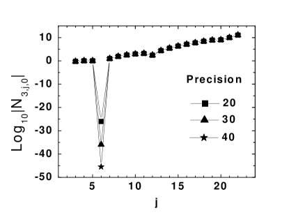
FIG. 1.: $Log_{10}(|N_{3,j,0}|)$ versus $j$.

In Figs. 2 and 3, we show $N_{l,i_{1},0}$ and $N_{l,i_{1},1}$ calculated with $pr$=20. One sees that $N_{2q+1,5q+1,0}$ and $N_{2q+2,5q,1}$ are more than 20 orders of magnitude smaller than the naive interpolation. We have checked in each of these cases that the small value drops by ten order of magnitudes each time the precision is increased just as in Fig. 1.

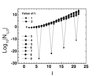
FIG. 2.: $Log_{10}(|N_{l,j,0}|)$ versus $j$ for $l=1,\dots 9$.

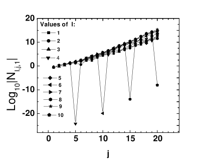
FIG. 3.: $Log_{10}(|N_{l,j,1}|)$ versus $j$ for $l=1,\dots 10$.

In summary, for each zero denominator considered, we found a zero numerator. We thus conjecture that all numerators corresponding to zero denominators are zero. If this conjecture is correct, the $s_{l,{\bf i}}$ corresponding to non-zero denominators are calculable from Eq. (10) and those corresponding to zero denominators are undetermined. The calculations performed above have been done with these coefficients treated as undetermined. The figures have been drawn with these coefficients set to zero. This choice is not essential, we have considered other choices where the undetermined coefficients have been set to values of the same order as the coefficients above and below (in $i_{1}$) and reached identical conclusions. This is a non-trivial statement. For instance, the undetermined coefficient $s_{3,6,0}$ appears explicitly in the numerator of the equation for $s_{5,11,0}$, however it is multiplied by a very small number which drops when $pr$ is increased.

We have checked that the individual terms in the zero numerators were not zero. The fact that we were able to obtain very precise cancellations without any fine-tuning suggests the existence of closed form formulas or of a symmetry forbidding these terms. More generally, the equally spaced spectrum (on a log scale), the number of terms at a given level $m$ (the order in HT expansion) equal to the number of partitions of $m$ [7] and the existence of “nested” ambiguities are somehow reminiscent of string theory. A possible starting point to discover these hypothetical symmetries would be to exploit the fact that since for instance $y_{3}$ and $y_{1}^{6}$ transform the same way under a RG transformation, there exist ambiguities in the construction of $h_{l}$ in terms of the scaling variables.

We should say a few words about the small denominators near other fixed points. The spectrum of the linearized RG transformation near the non-trivial fixed point [11] can be calculated numerically [16]. Investigating the small denominators of the form $\lambda_{l}^{k}\simeq\lambda_{m}^{r}$ for the first twenty eigenvalues and for powers not larger than 100. The best solution we found was $\lambda_{2}^{9}\simeq\lambda_{4}$ with two parts in a thousand. A more detailed study is necessary to decide if the rate of decay of the coefficients is sufficient to take care of the smaller denominator which will appear at larger orders. On the other hand, the spectrum at the Gaussian fixed point [9] is $\lambda_{j}=2c^{-j}$. There are many zero denominators in integer dimensions, e.g., $\lambda_{1}=\lambda_{2}^{2}$ for $D=3$. If the numerators are not zero, one can “repair” [1] the situation by considering $n$-dependent coefficients. This excludes a solution of the form of Eq. (7) but it generates logarithmic corrections which are necessary. These can even be observed in the large order of the HT temperature expansion in Ref. [17].

In conclusion, we have found remarkable cancellations of small denominators by small numerators. If these cancellations occur in general, it is possible to calculate analytically the thermodynamical quantities of Dyson’s hierarchical model in the HT phase using Eq. (10). Our results suggest that this model has features analogous to the integrable systems in Hamiltonian mechanics. As such, the model would stand out as a first approximation to be used in situations where the conventional perturbative expansions are not reliable.

This research was supported in part by the Department of Energy under Contract No. FG02-91ER40664. Y. M. thanks the Aspen Center for Physics for its hospitality in Summer 2000 while this work was in progress and for a conversation there with L. Kadanoff.

REFERENCES

- [1] F. Wegner, Phys. Rev. B 3, 4529 (1972).
- [2] F. Dyson, Comm. Math. Phys. 12, 91 (1969).
- [3] G. Baker, Phys. Rev. B 5, 2622 (1972).
- [4] A. Gonzalez-Arroyo and M. Okawa, Phys. Rev. D 35, 672 (1987).
- [5] P. de Forcrand et al., Nucl. Phys. B 577, 263 (2000).
- [6] K. Wilson, Phys. Rev. B. 4, 3185 (1971).
- [7] Y. Meurice and S. Niermann, u. of Iowa Preprint, hep-lat/00077037.
- [8] G. Baker and G. Golner, Phys. Rev. B 16, 2080 (1977).
- [9] P. Collet and J. Eckmann, A Renormalization Group Analysis of the Hierarchical Model in Statistical Mechanics (Springer-Verlag, Berlin, 1978).
- [10] P. Bleher and Y. Sinai, Comm. Math. Phys. 45, 247 (1975).
- [11] H. Koch and P. Wittwer, Math. Phys. Electr. Jour. 1, Paper 6 (1995).
- [12] Y. Meurice, G. Ordaz, and V. G. J. Rodgers, Phys. Rev. Lett. 75, 4555 (1995).
- [13] J. Godina, Y. Meurice, M. Oktay, and S. Niermann, Phys. Rev. D 57, 6326 (1998).
- [14] J. J. Godina, Y. Meurice, and M. Oktay, Phys. Rev. D 61, 114509 (2000).
- [15] Y. Meurice and S. Niermann, Phys. Rev. E 60, 2612 (1999).
- [16] J. Godina, Y. Meurice, and M. Oktay, Phys. Rev. D 57, R6581 (1998).
- [17] J. J. Godina, Y. Meurice, and S. Niermann, Nucl. Phys. B 519, 737 (1998).