On the Dynamics of the Evolution of HIV Infection

Abstract

We use a cellular automata model to study the evolution of HIV infection and the onset of AIDS. The model takes into account the global features of the immune response to any pathogen, the fast mutation rate of the HIV and a fair amount of spatial localization. Our results reproduce quite well the three-phase pattern observed in T cell and virus counts of infected patients, namely, the primary response, the clinical latency period and the onset of AIDS. We have also found that the infected cells may organize themselves into special spatial structures since the primary infection, leading to a decrease on the concentration of uninfected cells. Our results suggest that these cell aggregations, which can be associated to syncytia, leads to AIDS.

The human immunodeficiency virus (HIV), which causes AIDS (the acquired immunodeficiency syndrome) has been the subject of most intense studies, that encompass diverse fields of scientific research, ranging from the natural to the social sciences. Major progress has been achieved by medical and biological researchers in understanding the genetic code of the virus, the role of its high mutation rate, the virus-host interaction, the apparent failure of the immune system to control and eliminate the virus, and the onset of AIDS. Nevertheless, the mechanisms by which HIV causes AIDS still remain unexplained.

The immune response to any virus pathogen (virus, bacteria, etc.) is generated by a complex web of interactions, involving the cooperative and collective behavior of different types of white blood cells (monocytes, T- and B-cells). The time scale involved to develop a specific immune response may vary from days to weeks. The complex dynamic of HIV infection and the ensuing onset of AIDS involves a wide range of time scales [2]. The primary infection exhibits the same characteristics as any other viral infection: a dramatic increase of the virus population during the first $2-6$ weeks, followed by a sharp decline, due to the action of the immune system. For HIV, however, instead of being completely eliminated after the primary infection, a low virus burden is detected for a long asymptomatic time: the clinical latency period. This period may vary from two to ten (or more) years, depending on the patient. Besides the low concentration of HIV detected during this period, a gradual deterioration of the immune system is manifested by the reduction of CD4⁺T-cell populations in the peripheral blood. The third phase of the disease is achieved when the concentration of the T-cells is lower than a critical value ($\sim 30\%$), leading to the development of AIDS. As a consequence, the patient normally dies from opportunistic diseases, which would be usually controlled by the immune system. This common pattern observed during the course of the HIV infection [2] is depicted in Fig. 1, which shows the plasma viremia titer and the CD4⁺T cell counts in the peripheral blood as functions of time.

Several theories[3] have been proposed to explain why and how the virus remain (albeit in low concentrations) in the organism after the primary immune response, and the causes of the decline of T-cell counts, leading to the onset of AIDS. So far, none of them has provided, a complete explanation for the entire process. The most common assumption made to explain the permanence of the virus is that of fast mutation rate of the HIV, due to its rapid replication and its high degree of variability [4, 5]. This assumption plays a central role in our theory as well.

The challenge to understand the dynamics of the HIV infection has also attracted the attention of mathematicians and physicists that have been working on mathematical models [6] to describe different aspects of the dynamics of the host-parasite interaction. Although many of these models have contributed to the understanding of various aspects of the development of the disease, they fail to describe either the changes in the amount of virus detected in the body (blood, tissues and other body fluids) during the entire process or the two time scales observed in the course of the HIV infection, i.e., the primary response which runs from days to weeks and the clinical latency period that may vary from months to years. From the dynamical point of view, these different time scales may be related to two distinct kinds of interactions: one local and fast; and the other long-ranged and slow.

Most of the mathematical models proposed so far use population equations, treating the infected patient as a homogenous entity. Therefore local interactions and spatial inhomogeneities, caused by localization of the initial of immune response in lymphoid organs, are not taken into account. We believe that this feature, which is a natural ingredient of our model, are of central importance.

Experimental evidences [7] support that the lymphoid tissue is a major reservoir of HIV infection in vivo. Moreover a snapshot of the distribution of cells among the different compartments of the immune system will show only a small fraction ($2-4\%$) of the cells circulating in blood and lymph, while the majority is found in the lymphoid organs [8]. Paradoxically, the process of mobilization and activation of immune cells directed against the virus by the immune system, which occurs in the lymphoid micro-environment in this case, provides a milieu that contributes to the virus spread. [7].

Such spatial structure emerges naturally in discrete models, based on cellular automata that were shown [9] to describe well cooperative and collective patterns in experimentally observed immune response [10]. Therefore we model the course of the HIV infection by a cellular automaton. Our model takes into account the main features of the immune response to any pathogen, the high mutation rate of the HIV and a fair amount of spatial localization that may occur in the lymphoid tissues. Our aim is to test whether the combination of these hypotheses can explain the three-phase dynamics observed on the course of the HIV infection (see Fig. 1). The results obtained by simulations of our model are shown in Fig. 2 and, as far as we know, this is the first time that the complex dynamics of the HIV infection process has been so faithfully reproduced by a theoretical model.

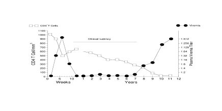
FIG. 1.: The common pattern exhibited by infected patients, first presented by Pantaleo et al [2]. The plasma viremia titer (black circles) and $CD4^{+}T$ cell counts (squares) versus time show a three-phase dynamics.

We model the immune system cells in the lymphoid tissues by a two-dimensional cellular automaton. To each lattice site we associate a cell, that may be a target for the HIV (as for instance, a CD4+T cell or a monocyte). Each cell can be in one of four states: (a) healthy; (b) infected-A1, corresponding to an infected cell that is free to spread the infection; (c) infected-A2, an infected cell against which a specific immune response has already developed and, finally (d) dead, an infected cell that was eliminated by the immune response.

The initial configuration is mainly composed of healthy cells, with a small fraction, $p_{HIV}$, of infected-A1 cells, representing the initial contamination by the HIV. In one time step the entire lattice is updated in a synchronized parallel way, according to the rules described below. The updated state of a cell depends on the states of its eight nearest neighbors.

Rule 1: Update of a healthy cell: (a): if it has at least one infected-A1 neighbor, it becomes infected-A1. (b): if it has no infected-A1 neighbor but does have at least $R$ ($2<R<8$) infected-A2 neighbors, it becomes infected-A1 (c): otherwise it stays healthy.

Rule 1a mimics the spread of the HIV infection by contact, before the immune system had developed its specific response against the virus. Rule 1b represents the fact that infected-A2 cells may, before dying, contaminate a healthy cell if their concentration is above some threshold.

Rule 2: An infected-A1 cell becomes infected-A2 after $\tau$ time steps.

An infected-A2 cell is one against which the immune response has developed and hence its ability to spread the infection is reduced. Here $\tau$ represents the time required for the immune system to develop a specific response to kill an infected cell. Such a time delay is required for each infected cell since in our model we view each new infected cell as carrying a different lineage (strain) of the virus. This is the way we incorporate the fast mutation rate of the virus in our model. When a healthy cell is infected, the virus uses the cell’s DNA in order to transcribe its RNA and replicate. During each transcription an error may occur, producing, on the average, one mutation per generation and hence a new strain of the virus is produced [4, 5].

Rule 3: Infected-A2 cells become dead cells.

This rule simulates the depletion of the infected cells by the immune response.

Rule 4: (a) Dead cells can be replaced by healthy cells with probability $p_{repl}$ in the next time step, (or remain dead with probability $1-p_{repl}$). (b) Each new healthy cell introduced may be replaced by an infected-A1 with probability $p_{infec}$.

Rule 4a describes the bone marrow replenishment of the depleted cells, mimicking the high ability of the immune system to recover from the immunosupression generated by infection. As a consequence, it will also mimic some diffusion of the cells in the tissue. Rule 4b simulates the entrance of new infected cells in the system that could come from other compartments of the immune system.

This four-state automaton allows transitions from each of its four states into the next one in a cyclic manner. We performed simulations of the model on square lattices with periodic boundary conditions of $N=L^{2}$ sites, with $L$ ranging from $300$ up to $1000$. All the parameters adopted in the simulations were based on experimental data. The initial concentration of HIV, $p_{HIV}=0.05$, was chosen based on the observation that the order of one in $10^{2}$ or $10^{3}$ T cells harbor viral DNA during the primary infection [11]. We adopted $p_{infec}=10^{-5}$ due to the fact that only one in $10^{4}$ to $10^{5}$ cells in the peripheral blood of infected individual express viral proteins. Since the immune system has a high ability to replenish the depleted cells, we used $p_{repl}=0.99$, although smaller probabilities could also be considered, representing different individuals. Since the time delay parameter ($\tau$) may vary from $2$ to $6$ weeks, we chose $\tau=4$. Each of our time steps corresponds to one week.

We present in Fig. 2 the evolution of the densities of healthy cells, infected cells (considering both A1 and A2 types) and dead cells, obtained in simulations of our model . We show results averaged over one hundred simulations (that used different initial configurations) and the corresponding standard deviations (shown as error bars). There is excellent qualitative agreement between our results for the density of healthy and infected cells and the time evolution of the number of CD4+ T cells in the peripheral blood and the plasma viremia titer showed in Fig. 1. The model reproduces the two time scales observed in the dynamics of the HIV infection: a short one associated with the primary infection and a long one related to the clinical latency period and the onset of AIDS. The small error bars related to the first stage of the infection indicated that its dynamics is insensitive to the initial configuration. However, the large error bars during the latency period suggest the presence of some mechanism regulating this phase of infection.

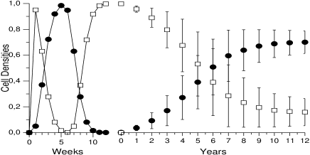
FIG. 2.: The results obtained from our simulations for a two-dimensional lattice with $L=700$, $p_{HIV}=0.05$, $R=4$, $\tau=4$, $p_{infec}=10^{-5}$, $p_{repl}=0.99$. The evolution of the population densities exhibit the same three-phase dynamics observed for infected patients. We have adopted open squares for healthy cells, full circles for infected cells.

The results presented in Fig. 2 are global properties, i.e. average quantities over the entire system. Our model allows also a closer look at local behavior, which in fact, may provide the clue for understanding also the global properties. From the analysis of the spatial configurations generated by the model in various individual simulations, we noticed that the slow dynamics observed in the latency period is related to the emergence, after completion of the primary response, of some special spatial structures of infected cells. These growing special structures spread the infection in such way that they slowly commit more and more healthy cells, segregating and trapping uninfected cells.

In Fig. 3 we present four “snapshots” of typical configurations obtained during one particular simulation. Starting form an initial configuration mostly composed of healthy cells (blue) with a random distribution of infected-A1 cells (yellow), in subsequent time steps each individual infected-A1 cell generates a pulse of infected cells, of width $(\tau+1)$, propagating in all directions. Whenever the average distance $\langle l_{1}\rangle$ between individual infected cells in the initial configuration is less than or equal $(2\tau+1)$, the independent pulses achieve a maximum coverage of the lattice. For $\tau=4$ the maximum coverage occurs after five weeks as shown in Fig. 3a. Note that the distribution of dead (red) cells corresponds to the initial configuration of infected cells. After that the concentration of infected cells decreases to a minimal value at $2(\tau+1)$ time steps, establishing the end of the primary infection phase ($10$ weeks, in this case).

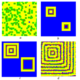
FIG. 3.: (Color) Four snapshots of parts of the lattice configuration for different time steps:(a)-(d) correspond to $5$, $18$, $25$ and $200$ weeks, respectively. During the latency period we observe an organization of different types of cells in layers which interpenetrate each other. We have adopted the same parameters used in Figure 2.

In the following time steps the presence of infected cells will be dictated by $p_{infec}$, according to rule 4b. When new infected cells are introduced, they may generate two different kinds of structures. The simplest case corresponds, as discussed above, to a wave of infected cells propagating in all directions, but in this case since $p_{infec}<<p_{HIV}$ the average distance $\langle l_{2}\rangle$ between the new infected cells, introduced with probability $p_{infec}$ at random locations, is much larger than $(2\tau+1)$. Examples of such structure are shown in the bottom right part of Figs. 3b and 3c. The spread of infection generated by these structures alone takes a longer time to reach nearly complete lattice coverage, and after that the infection vanishes. It is very rare, however, to find only these simple structures. A second type of structure also occurs, due to an interplay between rules 1b, 4a and 4b. These special structures are generated by ”sources” of infected cells. These sources appear, for instance, when a new infected-A1 cell, introduced by rules 4a and 4b, is surrounded by at least four dead cells. At every every ($\tau+3$) time steps they launch a propagating wave front of infected cells with width ($\tau+1$). The period of the wave fronts corresponds to the period of time the infected-A1 cell (source) remains in the same state ($\tau$) plus the three time steps to transition to types infected-A2, dead and healthy, in this sequence. Figs 3b and 3c (upper left) show the growing of such structures for two subsequent periods, corresponding respectively to $18$ and $25$ weeks. As these structures grow, the number of infected cells increases and the concentration of healthy cells decreases. Moreover they segregate and trap uninfected cells between two consecutive waves of infected cells. These special pattern of cell aggregations explain the slow decrease of T cells in infected patients during the latency period. These growing structures may eventually cover the entire lattice, with final densities of different cells evolving towards a steady state with average concentrations: $(\tau+1)/(\tau+3)$ for all the infected cells, and $1/(\tau+3)$ for both the dead and healthy cells. Note that the average density for healthy cells at the steady state is always lower than the observed critical value($\sim 30\%$) of CD4₊ T cells counts related to the onset of AIDS in infected patients, i.e, the system’s breakdown. Therefore the dynamics of real experimental data is related to the transient behavior of our model and not to its steady state. The long time scale, associated with this transient period that follows the primary infection, during which the model relaxes towards its steady state, corresponds to the clinical latency period.

Analysis of the source distribution at any given time shows that the latency period depends on $\langle l_{3}\rangle$, the average distance between sources and, consequently, on the probability of occurrence of sources ($\sim p_{repl}.p_{infec}.p_{HIV}$). Actually, since new sources can be released at any time step, the length of this transient time depends on the spatio-temporal average of the distance between sources.

In this work we have shown that our cellular automaton model reproduces quite well the three-stage dynamics observed in the course of the HIV infection, and the different time scales observed in this process. The short time scale, characteristic of the primary infection, increases when $\tau$ is increased or when $p_{HIV}$ decreases. The long time scale, responsible for the clinical latency period and the onset of AIDS, is associated with the emergence of special structures, that increase slowly the number of infected cells and confine healthy cells. This special pattern formation depends on the value of the parameter $R$ of rule 1b, $p_{repl}$ and $p_{infec}$. Smaller values of $p_{repl}$ enhance the presence of dead cells and favor the formation of the special growing structures. We have also performed a careful investigation of the parameter space, and found that three-phase dynamics is reproducible for a wide range of the parameters. The complete study of the parameter space, the detalied discussion of the necessary conditions to generate the special spatial structures and the role they play spreading the infection, is under preparation and will be published elsewhere.

The growing structures of infected cells may be associated with syncytia, the aggregation of cells observed experimentally, suggesting according to our results that they are responsible for the depletion of T cells leading to AIDS. These results actually corroborate some previous suggestions that syncytia are responsible for the permanence of the virus in the system, based on the analysis of the similarities between HIV infection and other diseases [3, 12].

Finally we emphasize that our cellular automaton model is, as far as we know, the first model which succeeded to reproduce the general features of the complex dynamics of the HIV infection, as observed in infected patients. This work further substantiates claims made in previous studies [10], that discrete models may be useful to describe emergent properties of complex biological systems, and to understand the mechanisms underlying its dynamical behavior. The reason for our success in describing the three-stage dynamics, whereas the other approaches fail, is that they do not take into account the spatial localization effects that play a major role on the course of the infection. A detailed study of the mechanisms underlying the dynamics described by our model may lead to new differential equation approaches, more suitable to describe the kind of dynamics observed in the course of HIV infection.

We thank Dr. M. Curié Cabral, I. Procaccia, S. Bocalletti, and J-P. Eckmann for enlightening discussions and to Borko Stǒsic for assistance with color graphics. RMZS’ thanks J.F. Fontanari for the hospitality during her visit to IFSC-USP, and FAPESP (project 99/09999-1) for supporting her stay. This work was partially supported by the Brazilian Agencies CNPq, CAPES, FINEP (under the grant PRONEX 94.76.0004/97) and FAPERJ.

REFERENCES

- [1] Permanent address: Instituto de Física, Universidade Federal Fluminense, Av. Litorânea s/n- CEP 24210-340-Niterói, Rio de Janeiro, Brazil.
- [2] G. Pantaleo, C. Graziozi and A. S. Fauci, New England J. of Med. 328, 327 (1993)
- [3] A. S. Fauci, Science 239, 617 (1988)
- [4] M. A. Nowak and A. J. Michael, Sci. American 273, 42, August 1995
- [5] W. C. Drosopoulos et al., J. Mol. Med. 76, 604 (1998).
- [6] A. S. Perelson and P. W. Nelson, SIAM Review, 41, 3 (1999), and references therein.
- [7] O. J. Cohen, G. Pantaleo, G. K. Lam and A. S. Fauci, Springer Seminars in Immunopathology 18, 305 (1997).
- [8] D. J. Steckel, J. Theor. Biol. 186, 491 (1997); D. J. Steckel et al, Immunol. Today 18, 216 (1997).
- [9] R. M. Zorzenon dos Santos, in Annual Reviews of Computational Physics VI, 159-202, ed. by D. Stauffer, World Scientific (1999).
- [10] R. M. Zorzenon dos Santos and A. T. Bernardes, Phys. Rev. Lett. 81, 3034 (1998).
- [11] S. M. Schnittman et al., Science 245, 305 (1998); S. M. Schnittman et al., Ann. Int. Med, 113, 438 (1990).
- [12] R. A. Weiss, Science 272, 1885 (1996).