Local structure study of $\bf In_{x}Ga_{1-x}As$ semiconductor alloys using High Energy Synchrotron X-ray Diffraction

Abstract

Nearest and higher neighbor distances as well as bond length distributions (static and thermal) of the $\rm In_{x}Ga_{1-x}As$ $(0\leq x\leq 1)$ semiconductor alloys have been obtained from high real-space resolution atomic pair distribution functions (PDFs). Using this structural information, we modeled the local atomic displacements in $\rm In_{x}Ga_{1-x}As$ alloys. From a supercell model based on the Kirkwood potential, we obtained 3-D As and (In,Ga) ensemble averaged probability distributions. This clearly shows that As atom displacements are highly directional and can be represented as a combination of $\langle 100\rangle$ and $\langle 111\rangle$ displacements. Examination of the Kirkwood model indicates that the standard deviation ($\sigma$) of the static disorder on the (In,Ga) sublattice is around 60% of the value on the As sublattice and the (In,Ga) atomic displacements are much more isotropic than those on the As sublattice. The single crystal diffuse scattering calculated from the Kirkwood model shows that atomic displacements are most strongly correlated along $\langle 110\rangle$ directions.

I Introduction

Semiconductor alloys are known as technologically important materials for their wide applications in optoelectronic devices such as lasers and detectors. [1] The local structure information is of fundamental importance in understanding the alloy systems because their physical properties are strongly influenced by the local atomic displacements present in the alloys. For example, it is known that chemical and compositional disorder strongly affect the electronic structure of zinc-blende type alloys [2, 3, 4, 5, 6, 7] and their enthalpies of formation. [8, 9]

In this paper we present a detailed study of the local and average structure of the $\rm In_{x}Ga_{1-x}As$ alloy series. The average structure of $\rm In_{x}Ga_{1-x}As$ was studied by Woolley. [10] The structure is of the zinc blende type ($F4\overline{3}m$) [11] over the entire alloy range. The lattice parameters, and therefore the average In-As and Ga-As bond lengths, interpolate linearly between the values of the end-members according to Vegard’s law. [12] However, consideration of the local structure reveals a very different situation. The local structure of $\rm In_{x}Ga_{1-x}As$ was first studied by Mikkelson and Boyce using extended x-ray absorption fine structure (XAFS). [13] According to this experiment, the individual nearest neighbor (NN) Ga-As and In-As distances in the alloys are rather closer to the pure Ga-As and In-As distances. Further XAFS experiments showed that this is quite general behavior for many zinc-blende type alloy systems. [14, 15, 16] Since then a number of theoretical and model studies have been carried out on the semiconductor alloys to understand how the alloys accommodate the local displacements. [17, 18, 19, 20, 21, 22, 23, 24]

Until now these models and theoretical predictions are tested mainly by the comparison with XAFS data. The XAFS results give information about the nearest neighbor and next nearest neighbor distances in the alloys but imprecise information about bond-length distributions and no information about higher-neighbor shells. This limited structural data makes it difficult to differentiate between competing models for the local structure. For example, even a simple radial force model [18] rather accurately predicts the nearest neighbor distances of $\rm In_{x}Ga_{1-x}As$ alloys in the dilute limit. Therefore, one needs more complete structural information including nearest neighbor, far-neighbor distances, and bond length distributions to prove the adequacy of model structures for these alloys.

The atomic pair distribution function (PDF), $G(r)$, measures the probability of finding an atom at a distance $r$ from another atom. [25] One of the advantages of the PDF method over other local probes such as XAFS is that it gives both local and intermediate range information because both Bragg peaks and diffuse scattering are used in the analysis. It is also possible to obtain information about the static bond length distribution from the PDF peak width and about correlations of atom displacements. [26]

In this paper, we present a detailed X-ray diffraction study of $\rm In_{x}Ga_{1-x}As$, $(0\leq x\leq 1)$. A preliminary analysis of the data has been published elsewhere. [27] Using high energy synchrotron x-rays, we measured the total scattering structure function, $S(Q)$, of the $\rm In_{x}Ga_{1-x}As$ alloy system extended to high $Q$ ($Q_{max}=45$ Å^-1) where $Q$ is the magnitude of the momentum transfer of the scattered x-rays ($Q=4\pi\sin\theta/\lambda$ for elastic scattering). From these structure functions we obtained the corresponding high real-space resolution PDFs through a Fourier transform according to

$$G(r)={{2\over\pi}\,\int^{\infty}_{0}Q[S(Q)-1]\sin\,Qr\,dQ}.$$ (1)

In these PDFs, the first peak is clearly resolved into two sub-peaks corresponding to the Ga-As and In-As bond lengths. [27] The evolution of the bond-length with doping gives good agreement with XAFS. For the far-neighbor peaks, the peak widths are much broader in the alloy samples than those of the pure end-members reflecting the increased disorder. We model the local structure of $\rm In_{x}Ga_{1-x}As$ alloys using a supercell model [28] based on the Kirkwood potential [29] which gives good agreement with the alloy data with no adjustable parameters. The results of the modeling have been analyzed to reveal the average atomic static distribution on the As and (In,Ga) sublattices. Finally, we have calculated the diffuse scattering that one would get from the Kirkwood model. This compares qualitatively well with published diffuse scattering results from $\rm In_{0.53}Ga_{0.47}As$. [30]

II Experimental details

A Data collection

The alloy samples, with compositions $\rm In_{x}Ga_{1-x}As$, (x = 0, 0.17, 0.33, 0.5, 0.83, 1) were prepared by a melt and quench method. An appropriate fraction of InAs and GaAs crystals were powdered, mixed and sealed under vacuum in quartz ampoules. The samples were heated beyond the liquidus curve of the respective alloy [10, 31] to melt them and held in the molten state for 3 hours before quenching them in cold water. The alloys were powdered, resealed in vacuum, and annealed just below the solidus temperature for 72-96 hours to increase the homogeneity of the samples. This was repeated until the homogeneity of the samples, as tested by x-ray diffraction, was satisfactory. X-ray diffraction patterns from all the samples showed single, sharp diffraction peaks at the positions expected for the nominal alloy similar to the results obtained by Mikkelson and Boyce. [13]

High energy x-ray powder diffraction measurements were conducted at the A2 wiggler beamline at Cornell High Energy Synchrotron Source (CHESS) using intense x-rays of 60 KeV ($\lambda=0.206$ Å). The incident x-ray energy was selected using a Si(111) double-bounce monochromator. All measurements were carried out in flat plate symmetric transmission geometry. In order to minimize thermal atomic motion in the samples, and hence increase the sensitivity to static displacements of atoms, the samples were cooled down to 10 K using a closed cycle helium refrigerator mounted on the Huber 6 circle diffractormeter. The samples were uniform flat plates of loosely packed fine powder suspended between thin foils of kapton tape. The sample thicknesses were adjusted to achieve sample absorption $\mu t\sim 1$ for the 60 KeV x-rays, where $\mu$ is the linear absorption coefficient of the sample and $t$ is the sample thickness.

The experimental data were collected up to $Q_{max}=45$ Å^-1 with constant $\Delta Q$ steps of 0.02 Å^-1. This is a very high momentum transfer for x-ray diffraction measurements. For comparison, $Q_{max}$ from Cu $K_{\alpha}$ x-ray tube is less than 8 Å^-1. This high $Q_{max}$ is crucial to resolve the small difference ($\approx 0.14$ Å) in the In-As and Ga-As bond lengths.

To minimize the measuring time, the data were collected in two parts, one in the low $Q$ region from 1 to 13 Å^-1 and the other in mid-high $Q$ region from 12 to 50 Å^-1. Because of the intense scattering from the Bragg peaks, in the low $Q$ region the incident beam had to be attenuated using lead tape to avoid detector saturation. The maximum intensity was scaled so that the count rate across the whole detector energy range in the Ge detector did not exceed $\sim 2\times 10^{4}~{}s^{-1}$. At these count-rates detector dead-time effects are significant but can be reliably corrected as we describe below. To reduce the random noise level below 1%, we repeated runs until the total elastic scattering counts become larger than 10,000 counts at each value of $Q$. Also, to obtain a better powder average the sample was rocked with an amplitude of $\pm 0.5^{\circ}$ at each $Q$-position. The scattered x-rays were detected using an intrinsic Ge solid state detector. The signal from the Ge detector was processed in two ways. The signal was fed to a multi-channel analyzer (MCA) so that a complete energy spectrum was recorded at each data-point. The signals from the elastic and Compton scattered radiation could then be separated using software after the measurement. In parallel, the data were also fed through single-channel pulse-height analyzers (SCA) which were preset to collect the elastic scattering, Compton scattering, and a wider energy window to collect both the elastic and Compton signals. For normalization, the incident x-ray intensity was monitored using an ion chamber detector containing flowing Ar gas.

For the SCAs, the proper energy channel setting for the elastic scattering is crucial. Any error in the channel setting could cause an unknown contamination by Compton scattering and make data corrections very difficult. There’s no such problem in the MCA method since the entire energy spectrum of the scattered radiation is measured at each value of $Q$. The main disadvantage of the MCA method is that it has a larger dead-time, although this can be reliably corrected as we show below. Fig. 1 shows a representative MCA spectrum

FIG. 1.: MCA spectrum of $\rm InAs$ at Q=45 Å^-1. Peaks in the spectrum from the elastic and Compton scattering are labelled, as is a peak from an electronic pulser used for dead-time correction. The other peaks in the spectrum come from various fluorescence and escape peaks.

taken from the InAs sample at $Q=45$ Å. It is clear that the Compton and elastic scattering are well resolved at this high momentum transfer. The elastically scattered signal, which contains the structural information, is obtained by integrating the area under the elastic scattering peak.

B Data Analysis

The measured x-ray diffraction intensity may be expressed [32] by

$$I^{mea}(Q)=PA[N(I^{coh}_{eu}+I^{inc}_{eu}+I^{mul}_{eu})],$$ (2)

where P is the polarization factor, A the absorption factor, N the normalization constant, and $I^{coh}_{eu},\ I^{inc}_{eu},\ I^{mul}_{eu}$ are the coherent single scattering, incoherent (Compton), and multiple scattering intensities, respectively, per atom, in electron units. The total scattering structure function, $S(Q)$, is then defined as

$$S(Q)=[I^{coh}_{eu}-(\langle f^{2}\rangle-{\langle f\rangle}^{2})]/{\langle f\rangle}^{2},$$ (3)

where $\langle f\rangle=\langle f(Q)\rangle$ is the sample average atomic form factor and $\langle f^{2}\rangle$ is the sample average of the square of the atomic form factor. Therefore, to obtain $S(Q)$ from the measured diffraction data, we have to apply corrections such as multiple scattering, polarization, absorption, Compton scattering and Laue diffuse corrections on the raw data. [32, 33]

The corrections were carried out using a home-written computer program, PDFgetX [34] that is able to utilize the MCA data. The results obtained using the MCA approach are very similar to those obtained using the SCA approach. [27] It appears that both approaches work well for quantitative high energy x-ray powder diffraction. One possible advantage of the MCA method is that energy windows of interest can be set after the experiment is over which is precluded if data are only collected using SCA’s.

We briefly describe some of the features of the data correction using PDFgetX. Data are first corrected for detector dead-time. In this experiment, we used the pulser method. [35] A pulse-train from an electronic pulser of known frequency is fed into the detector preamp. The voltage of the pulser pulses are set so that the signal appears in a quiet region of the MCA spectrum. The measured counts in the pulser signal in the MCA (or, indeed, in an SCA window set on the pulser signal) is then recorded for each data point. The data dead-time correction is then obtained by scaling the raw data by the ratio of the known pulser frequency and the measured pulser counts. This method accounts for dead-time in the preamp, amplifier and MCA/SCA electronics but not in the detector itself. However, in general the dead-time is dominated by the pulse-shaping time in the amplifier or the analogue-digital conversion in the MCA or SCA and so this method gives rather accurate dynamic measurement of the detector dead-time. An alternative dead-time correction protocol for correcting MCA data is to use the MCA real-time/live-time ratio. This works reasonably well if the MCA conversion time is the dominant contribution to the detection dead-time. This approach gave similar results to the pulser correction in this case.

Multiple (mainly double) scattering can be a problem if samples are relatively thick and the radiation is highly penetrating as in the present case. The multiple scattering contribution contains no usable structural information and must be removed from the measured intensity. It depends on sample thickness and many other sample dependent factors such as attenuation coefficient, atomic number and weight of sample constituent. [36, 37, 38] It increases as the sample becomes thicker in both transmission and reflection geometry. The multiple scattering correction was calculated using the approach suggested by Warren [36, 37, 38] in the isotropic approximation. Calculation of the multiple scattering intensity is considerably simplified when the elastic and Compton signals are separated as is done here since only completely elastic multiple scattering events need to be considered. In $\rm In_{x}Ga_{1-x}As$ samples, the multiple scattering ratio was around 10$\%$ maximum at high $Q$ in transmission geometry. This result suggests that the proper multiple scattering correction becomes important in the high $Q$ region. Fig. 2 shows the double scattering ratio calculated for the $\rm In_{0.5}Ga_{0.5}As$ sample.

FIG. 2.: Calculated double scattering ratio, $I_{2}/I_{1}$ where $I_{2}$ is the intensity due to double scattering events and $I_{1}$ the single scattering intensity, for the $\rm In_{0.5}Ga_{0.5}As$ alloy in transmission geometry with a $\mu t=1.32$ appropriate for our sample.

The x-ray polarization correction is almost negligible for synchrotron x-ray radiation because the incident beam is almost completely plane polarized perpendicular to the scattering plane. As a result there is virtually no angle dependence to the measured intensity due to polarization effects. [36]

The Compton scattering correction is very important in high-energy x-ray diffraction data analysis. It can become larger than the coherent scattering intensity at high $Q$, as is evident in Fig. 1. Even a small error in determining the Compton correction can lead to a significant error in the coherent scattering intensity in the high $Q$ region. However, in this region of the diffraction pattern the elastic and Compton-shifted scattering are well separated in energy and can be reliably separated using the energy resolved detection scheme we used here. At low-$Q$ the Compton-shift is small and the Compton and elastic signals cannot be explicitly separated unless a higher energy resolution measurement is made, for example, using an analyzer crystal. However, the Compton intensity is much lower and the coherent scattering intensity is much larger. In this region a theoretically calculated Compton signal can be subtracted from the data containing both elastic and Compton scattering. Uncertainties in this process have a very small effect on the resulting $S(Q)$. Fig. 3 shows the signals from the Compton and elastic

FIG. 3.: Comparison between Compton and elastic scattering intensities measured in $\rm In_{0.5}Ga_{0.5}As$.

scattering in the $\rm In_{0.5}Ga_{0.5}As$ sample. At low $Q$, some contamination from the elastic scattering is apparent in the Compton channel. For the Compton scattering correction, we followed two steps. In the high $Q$ region the Compton scattered signal was directly removed by integrating a narrow region of interest in the MCA spectrum which only contained the elastic peak. In the low $Q$ region we calculated the theoretical Compton scattering [39, 40] and subtracted this from the combined (unresolved) Compton plus elastic scattering signal. These two regions were smoothly interpolated using a window function, following the method of Ruland [41] in which the theoretical Compton intensity is smoothly attenuated with increasing $Q$.

At very high $Q$ values, due to the Debye-Waller factor, the Bragg peaks in the elastic scattering signal disappear and the normalized intensity asymptotes to $\langle f(Q)^{2}\rangle$. This fact allows us to obtain an absolute data normalization by scaling the data to line up with $\langle f(Q)^{2}\rangle$ in the high-$Q$ region of the diffraction pattern. Finally, the total scattering structure function, $S(Q)$, is then obtained using Eq. 3 and the corresponding PDFs, $G(r)$ are obtained according to Eq. 1.

III Results

Fig. 4 shows the experimental reduced total scattering structure functions, $F(Q)=Q[S(Q)-1]$, for the $\rm In_{x}Ga_{1-x}As$ alloys measured at 10 K.

FIG. 4.: The reduced total scattering structure function $[S(Q)-1]Q$ for In_xGa_1-xAs measured at 10K. The data-sets are offset for clarity. The high-$Q$ region is shown on an expanded scale ($\times$ 3) to highlight the presence of diffuse scattering.

It is clear that the Bragg peaks are persistent up to $Q\sim 35$ Å^-1 in the end-members, GaAs and InAs. This reflects both the long range order of the crystalline samples and the small amount of positional disorder (dynamic or static) on the atomic scale. In the alloy samples, however, the Bragg peaks disappear at much lower $Q$-values but still many sharp Bragg peaks are present in the mid-low $Q$ region. Instead, oscillating diffuse scattering which contains local structural information is evident in high $Q$ region. The observation of Bragg peaks reflects the presence of long-range crystalline order in these alloys. The fact that the Bragg peak intensity disappears at lower $Q$-values in the alloys than the end-members reflects that there is significant atomic scale disorder in the alloys as expected. The oscillating diffuse scattering in the high-$Q$ region originates from the stiff nearest-neighbor In-As and Ga-As covalent bonds.

Fig. 5 shows the corresponding reduced PDFs, $G(r)$, obtained using Eq. 1.

FIG. 5.: The reduced PDF, $G(r)$ for In_xGa_1-xAs measured at 10 K. The data-sets are offset for clarity.

In the alloys, it is clear that the first peak is split into a doublet corresponding to shorter Ga-As and longer In-As bonds. [42] The position in $r$ of the left and right peaks does not disperse significantly on traversing the alloy series. This shows that the local bond lengths stay close to their end-member values and do not follow Vegard’s law, in agreement with the earlier XAFS[13] and PDF[27] reports. However, already by 10 Å the structure is behaving much more like the average structure. For example, the doublet of PDF peaks around 11 Å in GaAs (Fig. 5) remains a doublet (it doesn’t become a quadruplet in the alloys) and disperses smoothly across the alloy series to its position at around 12 Å in the pure InAs. This shows that already by 10 Å  the structure is exhibiting Vegard’s law type behavior.

It is also notable that for the nearest neighbor PDF peak, the peak widths are almost the same in both alloys and end-members but for the higher neighbors, the peaks are much broader in the alloys than in the end-members.

IV Atomic displacements in the alloys

A Modeling

A simplified view of the structural disorder in the $\rm A_{x}B_{1-x}C$ type tetrahedral alloys can be intuitively visualized by considering simple tetrahedral clusters centered about C sites (the unalloyed site). In the random alloy this site can have 4 A-neighbors (type-I), 3 A- and 1 B-neighbors (II), 2 A- and 2 B-neighbors (III), 1 A and 3 B-neighbors (IV) or 4 B neighbors (V). We assume that the mixed site (A,B) atoms stay on their ideal crystallographic positions. By considering each cluster type in turn we can predict the qualitative nature of the atomic displacements present in the alloy. Let the A atoms be larger than the B atoms.

FIG. 6.: Schematic diagram of As displacements in cluster (a) type II, (b) type III, and (c) type IV. Cluster types are discussed in the text. At the corner, large dark circle and small grey circle show In and Ga atom position respectively. At the center, the grey and dark circles correspond to the As atom position before and after displacement, respectively.

In clusters of type I and V the C atom will not be displaced away from the center of the tetrahedron. As is shown in Fig. 6, in type II clusters the C atom will displace away from the center directly towards the B atom. This is a displacement in a $\langle 111\rangle$ crystallographic direction. In type III clusters it will displace in a direction between the two B atoms along a $\langle 100\rangle$ crystallographic direction. Finally, in type IV clusters it will again be a $\langle 111\rangle$ type displacement but this time in a direction directly away from the neighboring A atom. Such a cluster model was used to make quantitative comparisons with the nearest neighbor bond distances observed in XAFS measurements[13] over the whole alloy series.[14] However, it was later shown that the agreement was largely accidental due to the boundary conditions chosen that all the clusters should have the average size determined from Vegard’s law.[17] Nonetheless, it is interesting to compare the prediction of this simple cluster model with the nearest-neighbor PDF peaks measured here since, for the first time, we have an accurate measurement of the bond length distributions as well as the bond lengths themselves.

Each cluster is independently relaxed according to the prescription of Balzarotti et al. [14] to get the bond-lengths within each cluster type. Assuming a random alloy the number of each type of cluster that is present can be estimated using a binomial distribution. This gives the static distribution of bond lengths predicted by the model. These are then convoluted with the broadening expected due to thermal motion. This was determined by measuring the width of the nearest neighbor peaks in the end-member compounds, InAs and GaAs. The result is shown in Fig. 7(a). It is clear that, although the

FIG. 7.: Comparison between Experimental PDF (open circles) and model PDF (solid line) for $\rm In_{0.5}Ga_{0.5}As$. (a) Tetrahedral cluster model with no disorder present on (In,Ga) sublattice. The sub-peaks represent the contributions from each type of cluster. Type I ($\times$), type II ($\Box$), type III ($\Diamond$), type IV ($\triangle$), and type V($\ast$). (b) The model PDF is calculated in the Pauling limit. The peak positions were obtained from the InAs and GaAs bond lengths in the end-members (solid line) and the InAs and GaAs bond lengths in the $\rm In_{0.5}Ga_{0.5}As$ PDF (dashed line). See the text for details. (c) Kirkwood supercell model.

cluster model gets the peak positions reasonably correct as exemplified by the agreement it gets with XAFS data, [14] it does rather a poor job of explaining the shape of the measured pair distribution. The major discrepancy is that too much intensity resides at, or close to, the undisplaced position leading to an unresolved broad first PDF peak in sharp contrast to the measurement. In contrast, we show in Fig. 7(b) the nearest neighbor atomic pair distribution in the Pauling limit, [43] again broadened by thermal motion. The peak positions were obtained by using the bond-lengths of the end-member compounds. It is clear that this actually does a better job than the cluster model, though it slightly, and not surprisingly, overemphasizes the splitting. The dashed line in this figure shows the peak profile that we obtain if we make the assumption that the nearest neighbor bond length changes in the alloy as seen in the Z-plot, [13, 27] but there is no increase in the bond length distribution. Again, this gives rather good agreement emphasizing the fact that there is very little inhomogeneous strain to the covalent bond length due to the alloying. [27]

A better model for the structure of these alloys [27, 44] is obtained from a relaxed supercell of the alloy system using a Kirkwood potential. [29] The potential contains nearest neighbor bond stretching force constants $\alpha$ and force constants $\beta$ that couple to the change in the angle between adjacent nearest neighbor bonds. In this relaxed supercell model, the force constants were adjusted to fit the end-members [21] with $\alpha_{{\rm{Ga-As}}}$ = 96N/m, $\alpha_{{\rm{In-As}}}$ = 97N/m, $\beta_{{\rm{Ga-As-Ga}}}$ = $\beta_{{\rm{As-Ga-As}}}$ = 10N/m and $\beta_{{\rm{In-As-In}}}$ = $\beta_{{\rm{As-In-As}}}$ = 6N/m. The additional angular force constants required in the alloy are taken to be the geometrical mean, so that $\beta_{{\rm{Ga-As-In}}}$ = $\sqrt{(\beta_{{\rm{Ga-As-Ga}}}.\beta_{{\rm{In-As-In}}})}$. The PDFs for the alloys could then be calculated in a self-consistent way for all the alloys with no adjustable parameters. [44] In this model, the lattice dynamics are also included in a completely self-consistent way. Starting with the force constants and the Kirkwood potential, the thermal broadening of the PDF peaks at any temperature can be determined directly from the dynamical matrix and this is how the PDFs were calculated in the present case.[27] The model-PDF is plotted with the data in Fig. 8 with the nearest-neighbor peak shown on an expanded scale in Fig. 7(c). The excellent agreement with the data over the entire alloy range suggests that the simple Kirkwood potential provides an adequate starting point for calculating distorted alloy structures in these III-V alloys.

FIG. 8.: Comparison between Experimental PDF (open circles) and model PDF (solid line) for $\rm In_{x}Ga_{1-x}As$. The model was the Kirkwood supercell model. The parameters $\alpha$ and $\beta$ are refined from the end-members and the PDFs for the alloys shown here are then calculated with no adjustable parameters.

Note that in comparing with experiment, the theoretical PDF has been convoluted with a Sinc function to incorporate the truncation of the experimental data at $Q_{max}=45$ Å.

B 3-D atomic probability distribution

Now, we analyze the relaxed supercell of alloy system obtained using a Kirkwood potential to get the average three dimensional atomic probability distribution of As and (In,Ga) atoms. Fig. 9 shows iso-probability surfaces for the As site in the $\rm In_{x}Ga_{1-x}As$ alloy.

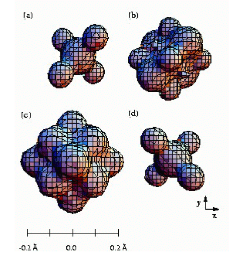
FIG. 9.: Iso-probability surface for the ensemble averaged As atom distribution. The surfaces plotted all enclose the volume where As atoms will be found with 68 % probability. (a) $\rm In_{0.17}Ga_{0.83}As$ (b) $\rm In_{0.33}Ga_{0.67}As$ (c) $\rm In_{0.50}Ga_{0.50}As$ (d) $\rm In_{0.83}Ga_{0.17}As$. In each case, the probability distribution is viewed down the [001] axis.

The probability distributions were created by translating atomic positions of the displaced arsenic atoms in the supercell ($20\times 20\times 20$ cubic cell) into a single unit cell. To improve statistics, this was done 70 times. The surfaces shown enclose a volume where the As atom will be found with 68 % probability. The probability distribution is viewed down the [001] axis. It is clear that the As atom displacements, though highly symmetric, are far from being isotropic. The same procedure has been carried out to elucidate the atomic probability distribution on the (In,Ga) sublattice. The results are shown in Fig. 10, plotted on the same scale as in Fig. 9.

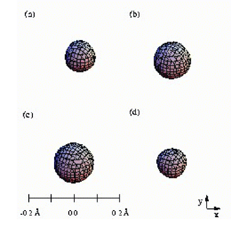
FIG. 10.: Iso-probability surface for the ensemble averaged (In,Ga) atom distribution. The surfaces plotted all enclose the volume where As atoms will be found with 68 % probability. (a) $\rm In_{0.17}Ga_{0.83}As$ (b) $\rm In_{0.33}Ga_{0.67}As$ (c) $\rm In_{0.50}Ga_{0.50}As$ (d) $\rm In_{0.83}Ga_{0.17}As$. In each case, the probability distribution is viewed down the [001] axis. These surfaces are plotted on the same scale as those in Fig. 9.

In contrast to the As atom static distribution, the (In,Ga) probability distribution is much more isotropic and sharply peaked in space around the virtual crystal lattice site.

In all compositions, the As atom distribution is highly anisotropic as evident in Fig. 9 with large displacements along $\langle 100\rangle$ and $\langle 111\rangle$ directions. This can be understood easily within cluster model as we discussed in Section IV A. The $\langle 100\rangle$ displacements occur in type III clusters and the $\langle 111\rangle$ displacements occur in type II and IV clusters. This also explains why, in the gallium rich alloy in which the three and four Ga cluster is dominant, the major As atom displacements are along [111], [1$\bar{1}\bar{1}$], [$\bar{1}$1$\bar{1}$], and [$\bar{1}\bar{1}$1] as we observed in Fig. 9(a). On the contrary, in the indium rich alloy, the major displacements are along [$\bar{1}\bar{1}\bar{1}$], [$\bar{1}$11], [1$\bar{1}$1], and [11$\bar{1}$], as can be clearly seen in Fig. 9(d).

The atomic probability distribution obtained from the Kirkwood model for the (In,Ga) sublattice is shown in Fig. 10. As we discussed, this is much more isotropic (though not perfectly so), and more sharply peaked than the As atom distribution. However, contrary to earlier predictions, [14] and borne out quantitatively by the supercell modeling, there is significant static disorder associated with the (In,Ga) sublattice. In order to compare the magnitude of the static distortion of the (In,Ga) sublattice with that of the As sublattice, we calculated the standard deviation, $\sigma$, of the As and (In,Ga) atomic probability distributions. This was calculated using $\sigma_{i}=\sqrt{{1\over{N-1}}\sum_{k=1}^{N}\,(d_{i}(k))^{2}},(i={x,y,z})$, where $d_{i}$ refers to the displacement from the undistorted sublattice of atoms in the model supercell in $x$, $y$, and $z$ directions, and $N$ is the total number of atoms in the supercell. Table I summarizes the values of $\sigma$ for the As and (In,Ga) atomic probability distributions in the alloys.

TABLE I.: Standard deviation of the As and (In,Ga) atom distributions in In_xGa_1-xAs alloys obtained from the Kirkwood model. The numbers in parentheses are the estimated error on the last digit. For both As, and (In,Ga) atoms, $\sigma=\sigma_{x}=\sigma_{y}=\sigma_{z}$. See text for details.

	x=0.17	x=0.33	x=0.50	x=0.83
$\sigma(As)$ (Å)	0.072(1)	0.092(1)	0.097(1)	0.074(1)
$\sigma(In,Ga)$ (Å)	0.044(1)	0.058(1)	0.060(1)	0.048(1)
${\sigma(In,Ga)\over\sigma(As)}$	0.61	0.63	0.62	0.61

It shows that for all compositions the static disorder on the (In,Ga) sublattice is around 60% of the disorder on the As sublattice. These static distortions give rise to a broadening of PDF peaks as described in Ref. 27 and evident in Fig. 5 of this paper. To evaluate the static contribution to the PDF peak broadening, $\sigma_{D}$, from the $\sigma^{\prime}s$ reported in Table I we used the following expression:

$$\sigma_{D}^{2}=\sigma_{a}^{2}+\sigma_{b}^{2},$$ (4)

where $a$, $b$ can be As, or (In,Ga). For example, for $x$ = 0.5 alloy, we get $\sigma_{D}^{2}$ = 0.0188(4) Ų for As-As peaks in the PDF, 0.0130(4) Ų for As-(In,Ga) peaks and 0.0072(3) Ų for (In,Ga)-(In,Ga) peaks. These values are in good agreement with the mean square static PDF peak broadening of As-As, As-(In,Ga) and (In,Ga)-(In,Ga) peaks, shown in Fig. 4 of Ref. 27, of 0.0187(1) Ų, 0.0128(1) Ų, and 0.0053(1) Ų respectively.

V Correlated atomic displacements

We have shown that on the average, atomic displacements of As atoms in $\rm In_{x}Ga_{1-x}As$ alloy are highly directional. In this section, we would like to address the question whether these atomic displacements are correlated from site to site. To investigate this we have calculated theoretically the diffuse scattering intensity which would be obtained from the relaxed Kirkwood supercell model and compare it with the known experimental diffuse scattering.

The Fig. 11 shows diffuse scattering of

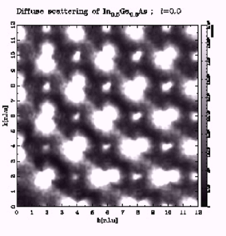
FIG. 11.: Single crystal diffuse scattering intensity obtained from the relaxed supercell model for the $\rm In_{0.5}Ga_{0.5}As$ alloy. The cut shown is the diffuse intensity expected in the $(hk0)$ plane of reciprocal space. Bragg peaks have been removed for clarity. See text for details.

$\rm In_{0.5}Ga_{0.5}As$ alloy calculated using the DISCUS program.[45] In this calculation the Bragg-peak intensities have been removed. Strong diffuse scattering is evident at the Bragg points in the characteristic butterfly shape pointing towards the origin of reciprocal space. This is the Huang scattering which is peaked close to Bragg-peak positions and has already been worked out in detail.[46]

In addition to this, clear streaks are apparent running perpendicular to the [110] direction. The diffuse scattering calculations on $(hkl)$ planes where $l\neq 0,\rm integer$ (Fig. 12),

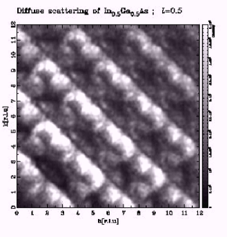
FIG. 12.: Single crystal diffuse scattering intensity obtained from the relaxed supercell model for the $\rm In_{0.5}Ga_{0.5}As$ alloy. The cut shown is the diffuse intensity expected in the $(hk0.5)$ plane of reciprocal space. Bragg peaks have been removed for clarity. See text for details.

show that these diffuse streaks are extended along the $[00l]$ direction consisting of sheets of diffuse scattering perpendicular to the [110] direction of reciprocal space. Diffuse scattering with exactly this (110) symmetry was observed in the TEM study of $\rm In_{0.53}Ga_{0.47}As$.[30] Careful observation of our calculated diffuse scattering indicates that the diffuse scattering has a maximum on the low-$Q$ side of the ($hk0$) planes passing through the Bragg points, with an intensity minimum on the high-$Q$ side of these planes. This is characteristic size-effect scattering obtained from correlated atomic displacements due to a mismatch between chemically distinct species as recently observed in a single-crystal diffuse scattering study on Si_1-xGe_x,[47] for example. This asymmetric scattering was clearly observed in the earlier diffuse scattering study on $\rm In_{0.53}Ga_{0.47}As$.[30]

The single-crystal diffuse scattering intensity which is piled up far from the Bragg-points is giving information about intermediate range ordering of the atomic displacements. It is interesting that it is piled up in planes perpendicular to [110] whereas the local atomic displacements are predominantly along $\langle 100\rangle$ and $\langle 111\rangle$ directions. This observation underscores the complementarity of single-crystal diffuse scattering and real-space measurements such as the PDF. The real-space measurements are mostly sensitive to the direction and magnitude of local atomic displacements and less sensitive to how the displacements are correlated over longer-range (though this information is in the data). On the other hand, the single crystal diffuse scattering immediately yields the intermediate range correlations of the displacements but one has to work harder to extract information about the size and nature of the local atomic displacements. Used together these two approaches, together with XAFS, can reveal a great deal of complementary information about the local structure of disordered materials.

The single crystal diffuse scattering suggests that atomic displacements are most strongly correlated (i.e., correlated over the longest range) along [110] directions although the displacements themselves occur along $\langle 100\rangle$ and $\langle 111\rangle$ directions. The reason may be that the zinc-blende crystal is stiffest along [110] directions because of the elastic anisotropy in the cubic crystal. This was shown for the case of InAs and was used to explain why the 5th peak in the PDF (coming from In-As next neighbor correlations along [110] direction) was anomalously sharp in both experiments and calculations.[26] If the material is stiffer in this direction, one would expect that strain fields from displacements will propagate further in these directions than other directions in the crystal correlating the displacements over longer range. These are consistent with the displacement pair correlation function calculation by Glas [48] which shows that the correlation along $\langle 110\rangle$ directions is larger than correlations along $\langle 100\rangle$ and $\langle 111\rangle$ and extends further.

VI conclusions

In conclusion, we have obtained high real-space resolution PDFs of $\rm In_{x}Ga_{1-x}As$ ($0\leq x\leq 1$) alloys using high energy synchrotron x-ray diffraction. For this purpose, we developed a data analysis technique adequate for high energy synchrotron x-ray diffraction. The PDFs show a clearly resolved doublet corresponding to the Ga-As and In-As bond lengths in the first peak of the alloys. Far-neighbors peaks are much broader in the alloys than that of the pure end members.

We show that As atom displacements are highly directional and can be represented as a combination of $\langle 100\rangle$ and $\langle 111\rangle$ displacements. On the contrary, the (In,Ga) atomic distribution is much more isotropic. The magnitude of (In,Ga) sublattice disorder is less than, but rather comparable ($\sigma_{(In,Ga)}\sim 0.6\sigma_{As}$) to, the As sublattice disorder. Also, the single crystal diffuse scattering shows that atomic displacements are correlated over the longest range in [110] directions although the displacements themselves occur along $\langle 100\rangle$ and $\langle 111\rangle$ directions.

All of the available data, including previous XAFS studies,[13] the present data,[27] differential PDF data,[42] and diffuse scattering on a closely related system[30] are well explained by a relaxed supercell model based on the Kirkwood potential.[44] This study also underscores the importance of having data from complementary techniques when studying the detailed structure of crystals with significant disorder.

- [1] A. M. Glass, Science 235, 1003 (1985).
- [2] A. Zunger and J. E. Jaffe, Phys. Rev. Lett. 51, 662 (1983).
- [3] K. C. Hass, R. J. Lempert, and H. Ehrenreich, Phys. Rev. Lett. 52, 77 (1984).
- [4] J. Hwang, P. Pianetta, Y.-C. Pao, C. K. Shih, Z.-X. Shen, P. A. P. Lindberg, R. Chow, Phys. Rev. Lett. 61, 877 (1988).
- [5] M. F. Ling, and D. J. Miller, Phys. Rev. B 38, 6113 (1988).
- [6] S. N. Ekpenuma, C. W. Myles, and J. R. Gregg, Phys. Rev. B 41, 3582 (1990).
- [7] Z. Q. Li, and W. Potz, Phys. Rev. B 46, 2109 (1992).
- [8] A. Silverman, A. Zunger, R. Kalish, and J. Adler, Phys. Rev. B 51, 10 795 (1995); A. Silverman, A. Zunger, R. Kalish, and J. Adler, Europhys. Lett. 31, 373 (1995).
- [9] L. Bellaiche, S.-H. Wei, and A. Zunger, Phys. Rev. B 56, 13 872 (1997).
- [10] J. C. Woolley, in Compound semiconductors, edited by R. K. Willardson and H. L. Goering Vol. 1, p. 3, New York, 1962, Reinhold Publishing Corp.
- [11] R. W. G. Wyckoff, Crystal Structures, Vol. 1, Wiley, New York, Second edition, 1967.
- [12] L. Vegard, Z. Phys. 5, 17 (1921).
- [13] J. C. Mikkelson and J. B. Boyce, Phys. Rev. Lett. 49, 1412 (1982); J. C. Mikkelsen and J. B. Boyce, Phys. Rev. B 28, 7130 (1983).
- [14] A. Balzarotti, N. Motta, A. Kisiel, M. Zimnal-Starnawska, M. T. Czyzyk, M. Podgorny, Phys. Rev. B 31, 7526 (1985); H. Oyanagi, Y. Takeda, T. Matsushita, T. Ishiguro, T. Yao, and A. Sasaki, Solid State Commun. 67, 453 (1988).
- [15] J. B. Boyce and J. C. Mikkelson, J. Cryst. Growth 98, 37 (1989).
- [16] Z. Wu, K. Lu, Y. Wang, J. Dong, H. Li, C. Li, and Z. Fang, Phys. Rev. B 48, 8694 (1993).
- [17] J. L. Martins and A. Zunger, Phys. Rev. B 30, 6217 (1984).
- [18] C. K. Shih, W. E. Spicer, W. A. Harrison, and A. Sher, Phys. Rev. B 31, 1139 (1985).
- [19] A.-B. Chen and A. Sher, Phys. Rev. B 32, 3695 (1985).
- [20] M. C. Schabel and J. L. Martins, Phys. Rev. B 43, 11 873 (1991).
- [21] Y. Cai and M. F. Thorpe, Phys. Rev. B 46, 15 879 (1992).
- [22] M. Podgorny, M. T. Czyzyk, A. Balzarotti, P. Letardi, N. Motta, A. Kisiel, and M. Zimnal-Starnawska, Solid State Commun. 55, 413 (1985).
- [23] A. Sher, Mark van Schilfgaarde, A.-B. Chen and W. Chen, Phys. Rev. B 36, 4279 (1987).
- [24] W. Zhonghua and L. Kunquan, J. Phys.: Condens. Matter 6, 4437 (1994).
- [25] S. J. L. Billinge and M. F. Thorpe, editors, Local structure from diffraction, New York, 1998, Plenum.
- [26] I.-K. Jeong, Th. Proffen, F. Mohiuddin-Jacobs, and S. J. L. Billinge, J. Phys. Chem. A. 103, 921 (1999).
- [27] V. Petkov, I.-K. Jeong, J. S. Chung, M. F. Thorpe, S. Kycia, and S. J. L. Billinge, Phys. Rev. Lett. 83, 4089 (1999)
- [28] J. S. Chung and M. F. Thorpe, Phys. Rev. B 55, 1545 (1997).
- [29] J. G. Kirkwood, J. Chem. Phys. 7, 506 (1939).
- [30] F. Glas, C. Gors, and P. Henoc, Philos. Mag. B 62, 373 (1990).
- [31] F. A. Cunnel, J. B. Schroeder in Compound semiconductors, edited by R. K. Willardson and H. L. Goering Vol. 1, p. 207 and 222, New York, 1962, Reinhold Publishing Corp.
- [32] Y. Waseda, The structure of non-crystalline materials, McGraw-Hill, New York, (1980).
- [33] C. N. J. Wagner, J. Non-Cryst. Solids 31, 1 (1978).
- [34] I.-K. Jeong, J. Thompson, A. Perez, Th. Proffen, and S. J. L. Billinge, unpublished.
- [35] O. U. Anders, Nucl. Instrum. Methods 68, 205 (1969).
- [36] B. E. Warren, X-Ray Diffraction, Dover, New York, 1990.
- [37] C. W. Dwiggins Jr and D. A. Park, Acta Crystallogr. A 27, 264 (1971); C. W. Dwiggins Jr, Acta Crystallogr. A 28, 155 (1972).
- [38] R. Serimaa, T. Pitkanen, S. Vahvaselka, and T. Paakkari, J. Appl. Crystallogr. 23, 11 (1990).
- [39] B. J. Thijsse, J. Appl. Crystallogr. 17, 61 (1984).
- [40] A. J. C. Wilson, editor, International tables for crystallography, Vol. C, 1995.
- [41] W. Ruland, Brit. J. Appl. Phys. 15, 1301 (1964).
- [42] V. Petkov, I.-K. Jeong, F. Mohiuddin-Jacobs, Th. Proffen and S. J. L. Billinge, J. Appl. Phys. 88, 665 (2000).
- [43] L. Pauling, The nature of the chemical Bond, Cornell Univ. Press, Ithaca, 1967.
- [44] J. S. Chung and M. F. Thorpe, Phys. Rev. B 59, 4807 (1999).
- [45] Th. Proffen, R. B. Neder, J. Appl. Crystallogr. 30, 171 (1997).
- [46] R. I. Barabash and J. S. Chung and M. F. Thorpe, J. Phys.: Condens. Matter 11, 3075 (1999).
- [47] D. Le Bolloc’h, J. L. Robertson, H. Reichert, S. C. Moss and M. L. Crow, unpublished.
- [48] F. Glas, Phys. Rev. B 51, 825 (1995).