Josephson currents through spin-active interfaces

Abstract

The Josephson coupling of two isotropic s-wave superconductors through a small, magnetically active junction is studied. This is done as a function of junction transparency and of the degree of spin-mixing occurring in the barrier. In the tunneling limit, the critical current shows an anomalous $T^{-1}$ temperature dependence at low temperatures and for certain magnetic realizations of the junction. The behavior of the Josephson current is governed by Andreev bound states appearing within the superconducting gap, $\Delta$, and the position of these states in energy is tunable with the magnetic properties of the barrier. This study is done using the equilibrium part of the quasiclassical Zaitsev-Millis-Rainer-Sauls boundary condition for spin-active interfaces and a general solution of the boundary condition is found. This solution is a generalization of the one recently presented by Eschrig [M. Eschrig, Phys. Rev B 61, 9061 (2000)] for spin-conserving interfaces and allows an effective treatment of the problem of a superconductor in proximity to a magnetically active material.

I Introduction

If a superconductor is exposed to magnetically active impurities[2, 3] or materials[4] the superconducting state is modified. Josephson coupling two superconductors through a magnetically active barrier may lead to what is known as a $"\pi"$-junction[3], a junction for which the ground state has an internal phase shift of $\pi$ between the superconductors across the barrier. If the barrier is extended to an S/F/S-structure, a ferromagnetic (F) layer sandwiched between two superconductors (S), the critical current will oscillate as the thickness of F is varied[4]. Additionally, the critical current will also depend on the strength of the exchange field in F. The principal reason for this strong dependence of junction properties is a drastic modification of the local superconducting density of states in the contact region to the F-layer [5]. Scattering of a magnetically active surface or transmission through a ferromagnetic barrier leads to a depairing of the Cooper-pairs and the creation of surface or layer Andreev states at energies within the superconducting gap. There have been an extensive experimental effort to explore the physics above by tunneling through magnetic insulator barriers[6, 7], by probing the proximity effect in S/F-structures[8] and constructing S/F-multilayers[9] (see also references therein). The problem at hand is quite formidable since the strength of the exchange energy is for most ferromagnetic materials, like Ni, Co and Fe, a sizable part of the Fermi energy $(\sim eV)$ while superconductivity lives on a much smaller energy scale $(\sim meV)$. To overcome the difference in energy scales the ferromagnetic layer must be extremely small $(\mathrel{\mathchoice{\lower 3.0pt\vbox{\halign{$\m@th\displaystyle\hfill#\hfil$\cr<\crcr\sim\crcr}}}{\lower 3.0pt\vbox{\halign{$\m@th\textstyle\hfill#\hfil$\cr<\crcr\sim\crcr}}}{\lower 3.0pt\vbox{\halign{$\m@th\scriptstyle\hfill#\hfil$\cr<\crcr\sim\crcr}}}{\lower 3.0pt\vbox{\halign{$\m@th\scriptscriptstyle\hfill#\hfil$\cr<\crcr\sim\crcr}}}}nm)$ and only recently have supercurrents been reported in S/F/S junctions by Veretennikov et al [10] using weak ferromagnetic alloys for the F-layer.

To efficiently model the S/F/S-junction there are two main routes of approach. The first is to assume an extension of a ferromagnetic metal, now characterized by a length and an exchange field, separating the two superconductors. Within this approach both critical current oscillations[4, 11] and the effect of the exchange field on the Andreev bound states[12, 13] have been studied. The limitation of the approach is that it is restricted to small exchange fields, i.e. fields that are comparable to the superconducting gap. An alternative approach is to treat the ferromagnetic part as a partially transparent barrier which transmits the two spin projections differently [3, 5, 14, 15]. Using Bogoliubov-deGennes equations and a WKB-approach for the ferromagnetic barrier[15], Josephson current-phase relations[16] and quasiparticle tunneling[17, 18] have been studied for both conventional s-wave and unconventional d-wave superconductors.

In this Paper, I follow the second path making use of the quasiclassical theory appropriate for describing low-energy phenomena like superconductivity for which considered energies are small compared to the Fermi energy $E_{F}$ [[19, 20, 21]]. Ferromagnetism will enter as a boundary problem for the quasiclassical Green’s functions $\hat{g}({\hat{\mbox{\boldmath$p$}}_{\!f}},{\mbox{\boldmath$R$}}_{s};\varepsilon)$ at a semi-transparent interface separating two conventional s-wave superconductors. There is no general restriction of validity of the present work to conventional superconductivity. The physics revealed in the simplest system proves to be quite rich without adding properties related to an unconventional pairing state[16, 17, 18] and therefore s-wave superconductivity in proximity to ferromagnetism should be studied in its own right. In section II, a general solution of the quasiclassical boundary condition, as posed by Millis, Rainer and Sauls [14], is given for equilibrium Green’s functions. In section III the local density of states in proximity to a ferromagnetic insulator is discussed. This is an important step in understanding the Josephson coupling between two s-wave superconductors studied as function of a simple phenomenological two spin-band scattering $\hat{S}$-matrix. Section IV is devoted to the study of the Josephson coupling and maps out regions where the junction is in a normal ”0”-state and where it switches to the ”$\pi$”-state.

II Boundary conditions for quasiclassical projectors at spin-active interfaces

Surfaces and interfaces involve energies of order $E_{F}$ which in quasiclassical theory[19] are integrated out at the onset. This means that boundary conditions for the quasiclassical Green’s function at surfaces and interfaces must be posed for the full Green’s function satisfying the Gor’kov equation. Resulting boundary conditions have then to be energy integrated into their quasiclassical form [22]. Physical properties of an interface can then be accounted for by a suitably chosen scattering S-matrix. A boundary condition for partially transmitting interfaces was first derived by Zaitsev [23] and, independently, by Kieselmann [24]. The boundary condition was later generalized by Millis, Rainer and Sauls (MRS) to include spin-active interfaces[14], i.e. interfaces which transmit and reflect quasiparticles differently depending on the spin projection.

Recently, Eschrig [25] used a projector method to solve Zaitsev’s boundary condition in general. The projectors, $\check{\cal P}^{(I)}_{\alpha}$, introduced relate to the quasiclassical Green’s function as $\check{g}^{(I)}=-i\pi(\check{\cal P}^{(I)}_{+}-\check{\cal P}^{(I)}_{-}).$ The superscripts $(I)$ label the side of the interface, the subscripts $\pm$ are directional indices and finally the ”háček” denote the Keldysh-matrix structure of the Green’s function. For a full account on the quasiclassical projectors $\check{\cal P}^{(I)}_{\alpha}$ and their parameterization, I refer the reader to Eschrig’s original paper[25] and in Appendix A I give a brief review of elements of quasiclassical theory used in this paper. Written in projectors $\check{\cal P}^{(I)}_{\alpha}$ equations (63-66) of MRS reads

  

$$\begin{array}[]{lr}\check{\cal P}^{(2)}_{-}\,\mbox{$\scriptscriptstyle\otimes$}\,\hat{S}_{22}\check{\cal P}^{(2)}_{+}\hat{S}_{22}^{\dagger}\,\mbox{$\scriptscriptstyle\otimes$}\,(\check{\cal P}^{(2)}_{-}-\check{1})&=\check{\cal P}^{(2)}_{-}\,\mbox{$\scriptscriptstyle\otimes$}\,\hat{S}_{21}\check{\cal P}^{(1)}_{-}\hat{S}_{21}^{\dagger}\,\mbox{$\scriptscriptstyle\otimes$}\,(\check{1}-\check{\cal P}^{(2)}_{-})\\[2.84544pt] \check{\cal P}^{(2)}_{+}\,\mbox{$\scriptscriptstyle\otimes$}\,\hat{S}_{22}^{\dagger}\check{\cal P}^{(2)}_{-}\hat{S}_{22}\,\mbox{$\scriptscriptstyle\otimes$}\,(\check{1}-\check{\cal P}^{(2)}_{+})&=\check{\cal P}^{(2)}_{+}\,\mbox{$\scriptscriptstyle\otimes$}\,\hat{S}_{12}^{\dagger}\check{\cal P}^{(1)}_{+}\hat{S}_{12}\,\mbox{$\scriptscriptstyle\otimes$}\,(\check{\cal P}^{(2)}_{+}-\check{1})\\[2.84544pt] (\check{\cal P}^{(1)}_{-}-\check{1})\,\mbox{$\scriptscriptstyle\otimes$}\,\hat{S}_{11}^{\dagger}\check{\cal P}^{(1)}_{+}\hat{S}_{11}\,\mbox{$\scriptscriptstyle\otimes$}\,\check{\cal P}^{(1)}_{-}&=(\check{1}-\check{\cal P}^{(1)}_{-})\,\mbox{$\scriptscriptstyle\otimes$}\,\hat{S}_{21}^{\dagger}\check{\cal P}^{(2)}_{-}\hat{S}_{21}\,\mbox{$\scriptscriptstyle\otimes$}\,\check{\cal P}^{(1)}_{-}\\[2.84544pt] (\check{1}-\check{\cal P}^{(1)}_{+})\,\mbox{$\scriptscriptstyle\otimes$}\,\hat{S}_{11}\check{\cal P}^{(1)}_{-}\hat{S}_{11}^{\dagger}\,\mbox{$\scriptscriptstyle\otimes$}\,\check{\cal P}^{(1)}_{+}&=(\check{\cal P}^{(1)}_{+}-\check{1})\,\mbox{$\scriptscriptstyle\otimes$}\,\hat{S}_{12}\check{\cal P}^{(2)}_{+}\hat{S}_{12}^{\dagger}\,\mbox{$\scriptscriptstyle\otimes$}\,\check{\cal P}^{(1)}_{+}\end{array}$$ (1)

  

Here, the non-commutative $\scriptscriptstyle\otimes$-product is a usual matrix product and a folding of internal energies. The solution of the system of equations (1) is facilitated by a convenient parameterization of $\check{\cal P}_{\alpha}$ in terms of four coherence functions $\gamma^{R},\tilde{\gamma}^{R},\gamma^{A},\tilde{\gamma}^{A}$ and two distribution functions $x^{K},\tilde{x}^{K}$. These six functions are 2$\times$2 spin matrices and superscripts (R,A,K) stand for Retarded, Advanced and Keldysh. The set of functions above obey Riccati-like equations that are easier to handle than the original quasiclassical matrix equation[25]. Especially, they fulfill certain stability criteria when integrated for along trajectories $x$. The functions $\gamma^{R},\tilde{\gamma}^{A}$ and $x^{K}$ are bounded when integrating the along a trajectory $({\mbox{\boldmath$v$}_{\!f}}({\hat{\mbox{\boldmath$p$}}})\cdot{\mbox{\boldmath$x$}}>0)$ and functions $\tilde{\gamma}^{R},\gamma^{A}$ and $\tilde{x}^{K}$ are bounded integrating in the opposite direction $({\mbox{\boldmath$v$}_{\!f}}({\hat{\mbox{\boldmath$p$}}})\cdot{\mbox{\boldmath$x$}}<0)$ [[26]]. Restating this in context of the interface problem we can always integrate up to the barrier obtaining $\gamma^{R},\tilde{\gamma}^{A}$, $x^{K}$ along trajectories with ${\mbox{\boldmath$v$}_{\!f}}({\hat{\mbox{\boldmath$p$}}})\cdot{\mbox{\boldmath$x$}}>0$, i.e. along the trajectories ${\hat{\mbox{\boldmath$p$}}}_{1}$ and ${\hat{\mbox{\boldmath$p$}}}_{2}$ in Figure 1. Similarly, $\tilde{\gamma}^{R},\gamma^{A}$ and $\tilde{x}^{K}$ are integrated stably along ${\mbox{\boldmath$v$}_{\!f}}(\underline{\hat{\mbox{\boldmath$p$}}})\cdot{\mbox{\boldmath$x$}}<0$, i.e. $\underline{\hat{\mbox{\boldmath$p$}}}_{1}$ and $\underline{\hat{\mbox{\boldmath$p$}}}_{2}$ in Figure 1. For constructing the Greens’s function at the surface that fulfills eqs. (1) we still need the ”scattered” functions $\Gamma^{R},\tilde{\Gamma}^{A}$ and $X^{K}$ with ${\mbox{\boldmath$v$}_{\!f}}(\underline{\hat{\mbox{\boldmath$p$}}})\cdot{\mbox{\boldmath$x$}}<0$ and $\tilde{\Gamma}^{R},\Gamma^{A}$ and $\tilde{X}^{K}$ with ${\mbox{\boldmath$v$}_{\!f}}({\hat{\mbox{\boldmath$p$}}})\cdot{\mbox{\boldmath$x$}}>0$. These functions have to be solved for from eqs. (1). Using the functions $(\gamma^{R}_{i},\tilde{\gamma}^{R}_{i},\Gamma^{R}_{i},\tilde{\Gamma}^{R}_{i})$, the Retarded projectors are constructed as

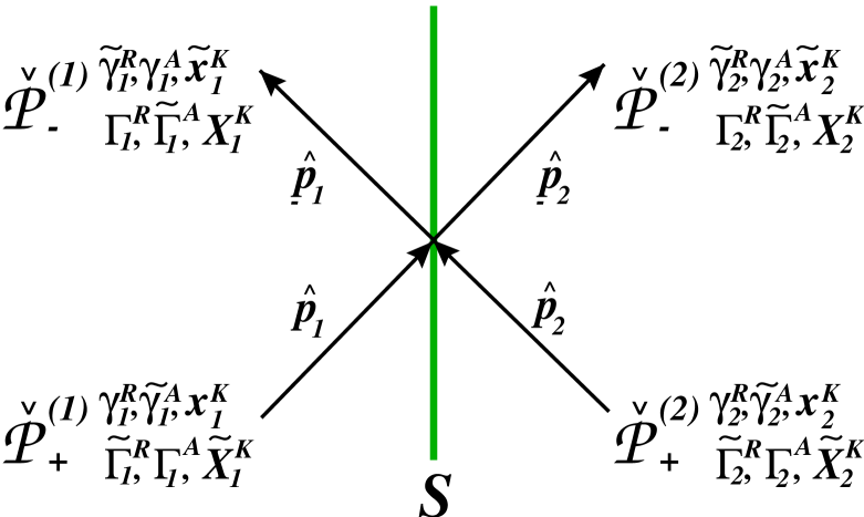
FIG. 1.: A schematic picture of the in-scattering trajectories $({\hat{\mbox{\boldmath$p$}}}_{1},{\hat{\mbox{\boldmath$p$}}}_{2})$ connected over an interface barrier parameterized by an S-matrix to the out-scattering ones $(\underline{\hat{\mbox{\boldmath$p$}}}_{1},\underline{\hat{\mbox{\boldmath$p$}}}_{2})$

$$\Bigg{\{}\begin{array}[]{l}\hat{\cal P}^{R}_{+}({\hat{\mbox{\boldmath$p$}}}_{1})=\left(\begin{array}[]{c}1\\ -\tilde{\Gamma}^{R}_{1}\end{array}\right)\mbox{$\scriptscriptstyle\otimes$}(1-\gamma^{R}_{1}\mbox{$\scriptscriptstyle\otimes$}\tilde{\Gamma}^{R}_{1})^{-1}\mbox{$\scriptscriptstyle\otimes$}\left(\begin{array}[]{c}1\,\,\,\gamma^{R}_{1}\end{array}\right)\\ \hat{\cal P}^{R}_{-}(\underline{\hat{\mbox{\boldmath$p$}}}_{1})=\left(\begin{array}[]{c}-\Gamma^{R}_{1}\\ 1\end{array}\right)\mbox{$\scriptscriptstyle\otimes$}(1-\tilde{\gamma}^{R}_{1}\mbox{$\scriptscriptstyle\otimes$}\Gamma^{R}_{1})^{-1}\mbox{$\scriptscriptstyle\otimes$}\left(\begin{array}[]{c}\tilde{\gamma}^{R}_{1}\,\,\,1\end{array}\right)\\ \end{array}$$

$$\Bigg{\{}\begin{array}[]{l}\hat{\cal P}^{R}_{+}({\hat{\mbox{\boldmath$p$}}}_{2})=\left(\begin{array}[]{c}-\gamma^{R}_{2}\\ 1\end{array}\right)\mbox{$\scriptscriptstyle\otimes$}(1-\tilde{\Gamma}^{R}_{2}\mbox{$\scriptscriptstyle\otimes$}\gamma^{R}_{2})^{-1}\mbox{$\scriptscriptstyle\otimes$}\left(\begin{array}[]{c}\tilde{\Gamma}^{R}_{2}\,\,\,1\end{array}\right)\\ \hat{\cal P}^{R}_{-}(\underline{\hat{\mbox{\boldmath$p$}}}_{2})=\left(\begin{array}[]{c}1\\ -\tilde{\gamma}^{R}_{2}\end{array}\right)\mbox{$\scriptscriptstyle\otimes$}(1-\Gamma^{R}_{2}\mbox{$\scriptscriptstyle\otimes$}\tilde{\gamma}^{R}_{2})^{-1}\mbox{$\scriptscriptstyle\otimes$}\left(\begin{array}[]{c}1\,\,\,\Gamma^{R}_{2}\end{array}\right)\\ \end{array}$$

and after substitution into eqs. (1) one finds after some straightforward algebra that the scattered-out functions can be expressed solely by scattering-in functions as

$$\begin{array}[]{ll}\Gamma^{R}_{1}&=(S_{11}\gamma^{R}_{1}\tilde{S}_{11}^{-1})\,\,\,\mbox{$\scriptscriptstyle\otimes$}\,\,{\cal{R}}^{R}_{1r}+(S_{12}\gamma^{R}_{2}\tilde{S}_{12}^{-1})\,\,\,\mbox{$\scriptscriptstyle\otimes$}\,\,{\cal{T}}^{R}_{1r}\\[2.84544pt] \tilde{\Gamma}^{R}_{1}&=(\tilde{S}^{\dagger}_{11}\tilde{\gamma}^{R}_{1}S^{\dagger-1}_{11})\,\mbox{$\scriptscriptstyle\otimes$}\,\,\tilde{\cal{R}}^{R}_{1r}+(\tilde{S}^{\dagger}_{21}\tilde{\gamma}^{R}_{2}S^{\dagger-1}_{21})\,\mbox{$\scriptscriptstyle\otimes$}\,\,\tilde{\cal{T}}^{R}_{1r}\end{array}$$ (8)

The generalized reflection coefficients ${\cal{R}}^{R}_{Sp}$ are defined as

$$\begin{array}[]{l}{\cal{R}}^{R}_{1r}=\tilde{S}_{11}\rho^{R-1}_{21}\,\mbox{$\scriptscriptstyle\otimes$}\,[\tilde{S}_{11}\rho^{R-1}_{21}-\tilde{S}_{12}\rho^{R-1}_{22}]^{-1}\\[2.84544pt] \tilde{\cal{R}}^{R}_{1r}=S^{\dagger}_{11}\tilde{\rho}^{R-1}_{12}\,\mbox{$\scriptscriptstyle\otimes$}\,[S_{11}^{\dagger}\tilde{\rho}^{R-1}_{12}-S^{\dagger}_{21}\tilde{\rho}^{R-1}_{22}]^{-1}\end{array}$$ (9)

and corresponding transmission coefficients ${\cal{T}}^{R}_{Sp}=1-{\cal{R}}^{R}_{Sp}$. The functions $\rho^{R}_{ij}$ and $\tilde{\rho}^{R}_{ij}$ are given as $\rho^{R}_{ij}=\tilde{S}_{ij}-\tilde{\gamma}^{R}_{i}\mbox{$\scriptscriptstyle\otimes$}S_{ij}\gamma^{R}_{j}\quad\mbox{and}\quad\tilde{\rho}^{R}_{ij}=S^{\dagger}_{ij}-\gamma^{R}_{j}\mbox{$\scriptscriptstyle\otimes$}\tilde{S}^{\dagger}_{ij}\tilde{\gamma}^{R}_{i}$. The scattered coherence functions on side 2 are given by interchanging the side index $1\leftrightarrow 2$. Advanced functions are related to the retarded ones by general symmetry $\hat{g}^{A}=\hat{\tau}_{3}(\hat{g}^{R})^{\dagger}\hat{\tau}_{3}$. The similarity in form of the final result given in equation (8) to the solution of a scattering problem is not a coincidence as the boundary condition for the quasiclassical Green’s function can also be solved by a direct scattering approach [27].

So far no reference to the form of the scattering $S$-matrix has been made. $S$ is a scalar in Keldysh space and a matrix ${\cal S}$ in particle-hole space, spanned by Pauli-matrices $\hat{\tau}_{j}$, with the form ${\cal S}=S(1+\hat{\tau}_{3})/2+\tilde{S}(1-\hat{\tau}_{3})/2$ where $\tilde{S}(p_{{}_{\parallel}})=S^{tr}(-p_{{}_{\parallel}})$ [[14]]. For spin-active interfaces the different components of the $S$-matrix, $S_{ij}$ in (8) above, are $2\times 2$ spin matrices. To proceed further a specific $S$-matrix is chosen to model the magnetic barrier

$$\hat{S}=\left(\begin{array}[]{cr}S_{11}&S_{12}\\ S_{21}&S_{22}\end{array}\right)=\left(\begin{array}[]{cr}r&t\\ t&-r\end{array}\right)\exp(i\Theta\sigma_{3})$$ (10)

where $\sigma_{j}$ notes the Pauli-matrices spanning spin space and parameters $(t,r)$ are the usual transmission and reflection coefficients. The S-matrix (10) is one of the simplest choices that allows a variable degree of spin mixing at the interface and the spin mixing is parameterized by the spin-mixing angle $\Theta$. By this construction $\hat{S}$ only violates spin conservation, i.e. it does not commute with the quasiparticle spin operator ${\sigma}$. The angle $\Theta$ will be considered as a phenomenological parameter independent of the trajectory direction in this paper, but as shown by Tokuyasu et al in the appendix of Ref. [[28]] one can relate $\Theta$ to the microscopic properties of the magnetic barrier. In particular, in Ref. [[28]] an S-matrix is constructed for a magnetically ordered insulating barrier and it is found, as expected, that $\hat{S}$ depends on the quasiparticle momentum projection parallel to the interface and on material parameters describing the barrier such as the average band gap, $E_{g}$, the internal exchange field, $h_{i}$, and its orientation $\hat{\mbox{\boldmath${\mu}$}}$.

Only the simplest case of an isotropic s-wave superconductor will be considered in this paper using weak coupling BCS theory. For this, assuming a constant order parameter in space $\Delta(x)=\Delta$, the retarded coherence functions are $\gamma^{R}=\gamma_{0}i\sigma_{2}$ and $\tilde{\gamma}^{R}=i\sigma_{2}\tilde{\gamma}_{0}$ with $\gamma_{0}=-\Delta/(\varepsilon^{R}+i\Omega)$, $\tilde{\gamma}_{0}=\Delta^{*}/(\varepsilon^{R}+i\Omega)$, $\Omega=\sqrt{|\Delta|^{2}-(\varepsilon^{R})^{2}}$ and $\varepsilon^{R}=\varepsilon+i\delta$. If, on the other hand, the effect of proximity to a magnetic material on the superconductor is of interest the Riccati equations[25]

$$\begin{array}[]{l}{i\,{\mbox{\boldmath$v$}_{\!f}}\!\!\cdot\!\!\mbox{\boldmath$\nabla$}_{\!\!{\mbox{\boldmath\mbox{$\scriptscriptstyle R$}}}}\,}\gamma^{R}+2\varepsilon^{R}\gamma^{R}=\gamma^{R}\tilde{\Delta}^{R}\gamma^{R}+\Sigma_{d}^{R}\gamma^{R}-\gamma^{R}\tilde{\Sigma}_{d}^{R}-\Delta^{R}\\ {i\,{\mbox{\boldmath$v$}_{\!f}}\!\!\cdot\!\!\mbox{\boldmath$\nabla$}_{\!\!{\mbox{\boldmath\mbox{$\scriptscriptstyle R$}}}}\,}\tilde{\gamma}^{R}-2\varepsilon^{R}\tilde{\gamma}^{R}=\tilde{\gamma}^{R}\Delta^{R}\tilde{\gamma}^{R}+\tilde{\Sigma}_{d}^{R}\tilde{\gamma}^{R}-\tilde{\gamma}^{R}\Sigma_{d}^{R}-\tilde{\Delta}^{R}\end{array}$$ (11)

have to be solved together with a self consistent determination of the order parameter $\hat{\Delta}(x)$ and of the impurity self energy $\hat{\Sigma}(x;\varepsilon)$ as described in the appendix. In eq. (11), $\Delta^{R}=\Delta+\Sigma^{R}_{od}$ and $\tilde{\Delta}^{R}=\tilde{\Delta}+\tilde{\Sigma}^{R}_{od}$ are the impurity renormalized gaps, while $\Sigma_{d}^{R}$ and $\tilde{\Sigma}_{d}^{R}$ are diagonal in Nambu space, and include both the impurity self energies $\Sigma_{\rm i}$ and the mean fields $\Sigma_{\rm m}$. All functions entering are spin matrices, and for the problems that will be considered in this paper it is sufficient to parameterize the matrices by two components as e.g. $(\gamma_{o}+\gamma_{3}\sigma_{3})i\sigma_{2}$ and $i\sigma_{2}(\tilde{\gamma}_{0}-\tilde{\gamma}_{3}\sigma_{3})$. The bulk values for $\gamma^{R}$ and $\tilde{\gamma}^{R}$, given above, serve in this case as initial values when integrating eqs. (11).

III Andreev bound states at an impenetrable magnetic barrier.

As a first point we return to the half-space model of Tokuyasu et al[28], a semi-infinite BCS-superconductor bounded by a magnetic insulator. The scattering off the insulator is assumed to be specular with a phase shift acquired differently at reflection for spin-up and spin-down quasiparticles. Using the $\hat{S}$-matrix above, the coherence functions scattered off the magnetic insulator are given directly by the incoming ones as $\Gamma=\exp{(i\Theta\sigma_{3})}\gamma_{0}i\sigma_{2}$ and $\tilde{\Gamma}=i\sigma_{2}\tilde{\gamma}_{0}\exp{(i\Theta\sigma_{3})}$. Using the information of the scattered coherence functions the Green’s function is given for a trajectory with $\hat{\mbox{\boldmath$n$}}\cdot{\hat{\mbox{\boldmath$p$}}_{\!f}}>0$ as

$$\hat{g}^{R}=-i\pi\;\hat{N}^{R}\left(\begin{array}[]{cc}(1+\gamma^{R}\tilde{\Gamma}^{R})&2\gamma^{R}\\ -2\tilde{\Gamma}^{R}&-(1+\tilde{\Gamma}^{R}\gamma^{R})\end{array}\right),$$ (12)

where

$$\hat{N}^{R}=\left(\begin{array}[]{cc}(1-\gamma^{R}\tilde{\Gamma}^{R})^{-1}&0\\ 0&(1-\tilde{\Gamma}^{R}\gamma^{R})^{-1}\end{array}\right).$$ (13)

If the trajectory is $\hat{\mbox{\boldmath$n$}}\cdot{\hat{\mbox{\boldmath$p$}}_{\!f}}<0$, the Green’s function is simply given by interchanging $\gamma\rightarrow\Gamma$ and $\tilde{\Gamma}\rightarrow\tilde{\gamma}$. The effect of the spin mixing is perhaps best seen in the spin and angle-resolved density of states (DOS) right at the barrier. On a trajectory with $\hat{\mbox{\boldmath$n$}}\cdot{\hat{\mbox{\boldmath$p$}}_{\!f}}>0$ this quantity is given by the imaginary part of $g^{R}({\hat{\mbox{\boldmath$p$}}_{\!f}},\varepsilon)$, the upper left component of (12) as described in eq. (A12). Assuming a constant order parameter up to the interface, the local DOS at the interface for spin-up quasiparticles, $N_{\uparrow}$, can be written as

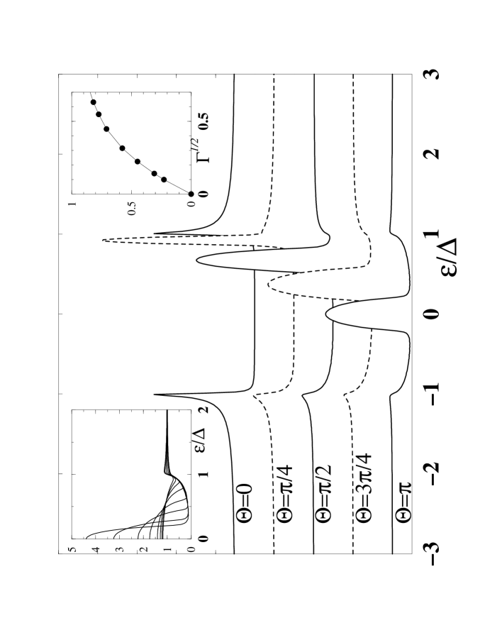
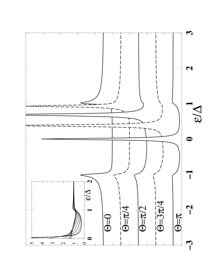
FIG. 2.: Tunneling density of states for spin-up quasiparticles at an impenetrable magnetically active insulator. The superconductor is a conventional BCS superconductor with a self consistently determined order parameter. In the main panels $\Theta$ is varied from 0 to $\pi$ in steps of $\pi/4$ going top to bottom and the curves are shifted for clarity. In the left figure the impurity scattering is in the Born limit while in the right panel the scattering is taken in the unitary limit. In both cases the scattering rate is chosen to $0.01$ in units of $2\pi T_{c}$. In the left inset in the left figure the DOS is plotted for $\Theta=\pi$ but with varying impurity scattering. The dependence of the zero-energy peak width with $\sqrt{\Gamma}$ is plotted in the right inset of the left panel. In the panel to the right the impurity scattering is in the unitary limit. As expected the broadening of the Andreev states is very much suppressed.

$$N_{\uparrow}({\hat{\mbox{\boldmath$p$}}_{\!f}},\varepsilon;\Theta)=Im\Bigg{[}\frac{\varepsilon^{R}\cos(\Theta/2)+\Omega\sin(\Theta/2)}{\Omega\cos(\Theta/2)-\varepsilon^{R}\sin(\Theta/2)}\Bigg{]}.$$ (14)

For spin-down quasiparticles $N_{\downarrow}$ reads the same after substitution $\Theta\rightarrow-\Theta$. This density of states has Andreev bound states inside the gap, i.e. for $|\varepsilon|<\Delta$. These states are located at $\varepsilon_{b,\uparrow(\downarrow)}=\pm\Delta\cos(\Theta/2)$, with $+(-)$ for the spin-up (-down) branch. It is notable that the DOS (14) has exactly the same form as the DOS calculated for a S/F/S weak link, for which the angle $\Theta$ is shown to depend on the thickness of and exchange field in the F-layer[29].

The existence of bound states will lead to a reduction of the order parameter amplitude in the vicinity of the magnetic interface. This is seen in Figure 2 in Ref. [[28]]. The pairbreaking occurs gradually as the bound state on either spin branch is tuned towards $\varepsilon_{b}=0$ with $\Theta\rightarrow\pi$. At $\Theta=\pi$ the order parameter is totally reduced at the interface and recovers to its bulk value over a distance of order $\xi_{o}$, the zero temperature coherence length in the superconductor. It turns out that the position in energy of the surface states, $\varepsilon_{b}$, is not to sensitive to a spatial variation in the order parameter. The Andreev bound states would be delta peaks if the superconductor had an infinite mean free path. The presence of impurities in the bulk give rise to a finite life time $\tau$ which broadens the Andreev peak. The broadening of the Andreev states is sensitive to the scattering strength of the impurities. In the main panels of the figures 2 the DOS is shown for different values of spin-mixing $\Theta$. The surface order parameter is self consistently determined for each spin-mixing angle. The scattering rate is $\Gamma=1/2\tau=0.01$ in units of $2\pi T_{c}$ and corresponds to a mean free path $\ell_{\rm{mfp}}=50\,\xi_{o}$. From the literature on d-wave superconductors it is known that surface bound states are broadened by impurity scattering as $\sim\sqrt{\Delta\Gamma}$ in the Born limit [30]. In the two insets in figure 2 the dependence of the width of the zero energy peak with scattering rate for $\Theta=\pi$ is shown. For small scattering rates indeed the $\sqrt{\Delta\Gamma}$-dependence is recovered. If, on the other hand, the scattering strength of the impurities is in the strong scattering limit the broadening of the Andreev bound states will be exponentially small, $\sim\sqrt{\Delta\Gamma}\exp[{-\Delta/\Gamma}]$ [[30]]. The effect of unitary scatterers is shown in the figure to the right in Fig. 2.

IV Josephson current-phase relation and the energy state of the junction.

Next, let us consider the Josephson current-phase relation through a magnetically active point contact. Assuming a point contact allows several simplifications. Effects of the contact itself on superconductivity i.e. the order parameter profile may be disregarded. This holds true if the contact radius is taken much smaller than the superconducting coherence length. Furthermore, spin-neutral surface scattering alone does not affect an isotropic s-wave superconductor and thus bulk values of the coherence functions $\gamma,\tilde{\gamma}$ can be used for the in-scattering ones in the boundary condition (8). An additional advantage of the point contact condition is that the results will not depend on the presence of non-magnetic bulk impurities as the current through the point contact depends only on bulk coherence functions. On the other hand, the point contact itself is fully described by its transmission $t$ and degree of spin mixing, $\Theta$. The Josephson current through the contact is calculated as a function of the phase difference, $\phi$, between two superconductors by the current formula

$${\mbox{\boldmath$j$}}(\phi)=eN_{f}\int^{\infty}_{-\infty}\frac{d\varepsilon}{8\pi i}{\rm Tr}\langle{\mbox{\boldmath$v$}_{\!f}}\hat{\tau}_{3}\hat{g}^{K}_{\phi}({\hat{\mbox{\boldmath$p$}}_{\!f}},0;\varepsilon)\rangle_{\hat{\mbox{\boldmath$p$}}_{\!f}}.$$ (15)

Here $\hat{g}^{K}_{\phi}({\hat{\mbox{\boldmath$p$}}_{\!f}},0;\varepsilon)=(\hat{g}^{R}_{\phi}({\hat{\mbox{\boldmath$p$}}_{\!f}},0;\varepsilon)-\hat{g}^{A}_{\phi}({\hat{\mbox{\boldmath$p$}}_{\!f}},0;\varepsilon))\tanh(\varepsilon/2T)$ is the equilibrium Keldysh Green function constructed from the retarded and advanced ones, $\hat{g}^{R,A}_{\phi}({\hat{\mbox{\boldmath$p$}}_{\!f}},0;\varepsilon)$, at the interface. Functions $\hat{g}^{R,A}_{\phi}({\hat{\mbox{\boldmath$p$}}_{\!f}},0;\varepsilon)$ are calculated at the interface so the boundary condition (8) is fulfilled. The resulting critical current of the junctions is characterized by different transparency and spin-mixing angle and show a rich variety as seen in Figures 3. This quantity is defined as the maximum amplitude of the current reached between a phase difference of $0$ and $\pi$. The sign of the critical current is either positive giving a $"0"$-junction or negative signaling a $"\pi"$-junction. For arbitrary transmission and spin mixing the analytic expression for the current is not very tractable and numerical analysis of the current-phase relation is more practical. In the two extreme limits of tunneling, $t<<1$, and high transparency, $t\simeq 1$, the analytical expression is simpler and reveals the physics going on.

Starting with the tunneling limit, the transmitted coherence functions $\Gamma,\tilde{\Gamma}$ as given by equations (8) are expanded to leading order in transparency ${\cal T}=|t|^{2}$. The expanded $\Gamma,\tilde{\Gamma}$ are then put into the expression for $\hat{g}^{R}$, eq. (12), and to first order in ${\cal T}$ the resulting current is given as follows

$$j(\phi;\Theta)={\cal T}j_{o}\sin\phi\,\int^{\infty}_{-\infty}\frac{d\varepsilon}{4\pi}\bigg{[}{\cal K}_{+}(\varepsilon,\Theta)+{\cal K}_{-}(\varepsilon,\Theta)\bigg{]}$$ (16)

where ${\cal K}_{\pm}(\varepsilon,\Theta)=[\Omega\cos(\Theta/2)\pm\varepsilon\sin(\Theta/2)]^{-2}\tanh(\frac{\varepsilon}{2T})$ and $j_{o}=2ev_{f}N_{f}\Delta^{2}$. In general the current is totally governed by the bound states at $\varepsilon_{b}=\pm\Delta\cos(\Theta/2)$ and their population at the given temperature $T$. Notable is that for all values of $\Theta$, the current-phase relation is sinusoidal. Setting $\Theta=0$ reproduces the usual Ambegaokar-Baratoff expression [31]. At $\Theta=\pi$, $\varepsilon_{b}$ is a zero-energy bound state and give rise to a $"\pi"$-junction with a critical current which increases as $T^{-1}$ with decreasing temperature as shown in the inset in the left figure 3. A similar anomaly in the critical current occurs for d-wave superconductors [32]. The difference between the anomaly in the two types of superconductors is that for d-wave superconductors any concentration of bulk impurities will give a finite width of the zero energy bound states and reduce the $T^{-1}$-anomaly. For an s-wave superconductor at a point contact only inelastic scattering processes, phase-breaking impurities or, as shown below, a finite ${\cal T}$ can give a similar broadening and the anomaly is quite robust due to long inelastic (phase-breaking) scattering times, i.e. $1/2\tau_{inel,(phase)}<<\Delta$. Going away from $\Theta=\pi$, $\varepsilon_{b}$ moves to finite energy and the functions ${\cal K}_{\pm}(\varepsilon,\Theta)$ acquire double pole structure at $\varepsilon_{b}$. The two poles are slightly shifted and have slightly asymmetric magnitude in residues. Given that the residues also are of different sign, they contribute oppositely to the critical current. The separation in energy of the poles is dependent on the imaginary part, $\delta$, of the energy $\varepsilon+i\delta$. $\delta$ can loosely be interpreted as an inelastic scattering rate. At $T=0$ and $\delta\rightarrow 0$ it turns out that the ground state of the junction is always a ”0”-junction except at $\Theta=\pi$. As temperature and/or the $\delta$ is increased the region in $\Theta$ showing a $"\pi"$-state junction increases. This is clearly demonstrated in figure 3 where the critical current is plotted as function of temperature. For all but the two largest values of $\Theta$ the low-T critical current is positive.

Sticking to the tunneling limit, the results derived here can also be obtained using equations (93-94) of MRS. What is crucial to note is that in order to find the bound state contribution to the current the Green’s functions must be the ones arrived at in eq. (12). This is taking into account the spatial dependence of the Green’s function at the magnetic pinhole, i.e. solving the impenetrable wall problem with the $\hat{S}$-matrix describing the pinhole. If this spatial dependence is neglected, and the bulk Green’s functions are used in equations (93-94) of MRS, the resulting Josephson current will simply have two contributions $\sin(\phi\pm\Theta)$, one contribution for each spin band.

Moving away from the tunneling limit the $T^{-1}$-anomaly is cut off by the finite value of ${\cal T}$. Instead, the switching between ”0” and $"\pi"$-states happens in abrupt jumps in the critical current. This abruptness is spurious since the current-phase relation has three zeros between 0 and $\pi$ and the change of state from $"\pi"$ to ”0” occurs without the current being zero for every phase difference. Instead the junction has two local minima in energy, at phase difference $\phi=0$ and $\pi$. Right at the switching point the two states are degenerate and the junction state can be tuned with temperature. This is shown in the inset of the middle figure 3 which depicts the junction energy vs. phase difference for a junction with ${\cal T}=0.1$ and $\Theta=3\pi/4$. As seen, between the two energy minima there is a potential barrier. This barrier is at highest at an intermediate phase $0<\phi<\pi$ where the current through the junction is zero. As temperature is swept over the switching temperature, which for this junction is at $T_{sw}\approx 0.12T_{c}$, the energy minimum jumps from $\phi=\pi$ to $\phi=0$ as temperature is increased through $T_{sw}$ and vice versa as the temperature is decreased through $T_{sw}$. The position in temperature depends on the two junction parameters ${\cal T}$ and $\Theta$. For larger transparencies the values of tunable junctions is restricted to a decreasing range in $\Theta$ just below $\Theta=\pi/2$.

If the transparency is taken to unity the tunability of the junction state with temperature vanishes. This is seen from the current-phase relation

$$j(\phi;\Theta)=j_{o}\int^{\infty}_{-\infty}\frac{d\varepsilon}{4\pi}\bigg{[}{\cal J}_{+}(\phi;\varepsilon,\Theta)+{\cal J}_{-}(\phi;\varepsilon,\Theta)\bigg{]}$$ (17)

with

$\displaystyle{\cal J}_{\pm}(\phi;\varepsilon,\Theta)={{\sin(\phi\pm\Theta)}\over{[\Omega^{2}-\varepsilon^{2}+\Delta^{2}\cos(\phi\pm\Theta)]}}\tanh(\frac{\varepsilon}{2T}).$

The current is now controlled by interface states located at $\varepsilon_{i}=\pm\Delta\cos[(\phi\pm\Theta)/2]$, i.e. at a position given by the phase $\phi$ but shifted by $\pm\Theta$ for the two spin bands as compared to the spin-neutral case. This shows up in the fact that at $\Theta=0$ the usual Kulik-Omel’yanchuk (KO) formula is recovered [33] and at finite $\Theta$, eq. (17) is a sum of two KO supercurrents evaluated at phases shifted by $\pm\Theta$. For spin-mixing angles $\Theta<\pi/2$ the junction is in the ”0”-state and at $\Theta>\pi/2$ in the $"\pi"$-state. At $\Theta=\pi/2$ the junction state is degenerate for every temperature as the current-phase relation has doubled periodicity.

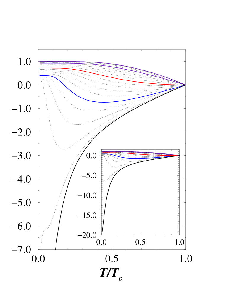
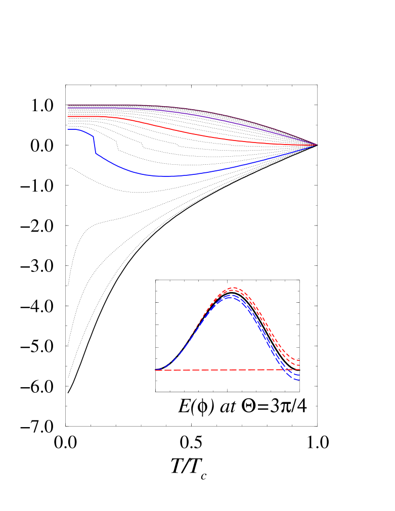
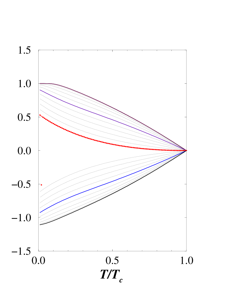
FIG. 3.: Critical currents for different transparencies $0.01,0.1$ and $0.99$, left to right, and for a dense sampling of the spin-mixing angle, $\Theta$ running from 0 to $\pi$ in steps of $\pi/20$. Thick lines are in intervals of $\pi/4$ as a guide for the eye. All currents are scaled with the value of the critical current at $T=0$ and $\Theta=0$ for the current value of ${\cal T}$. As is seen for all values of transparency, ${\cal T}$, the junction may either be a ”0” or a ”$\pi$”-junction depending on the degree of spin mixing. In the low transparency limit and at $\Theta=\pi$ the zero-energy bound state gives rise to a critical current $\sim T^{-1}$ as seen in the inset of the left most panel. At intermediate $\Theta$ the junction may switch between the ”0” and the ”$\pi$”-junction state with temperature. At larger ${\cal T}$ this switching becomes more abrupt in temperature. Finally, in the high transparency limit the switching between ”0” and the ”$\pi$”-junction state is lost and $\Theta$ defines the junction state for all temperatures.

V Discussion

In this paper a general solution is derived for the equilibrium part of the Zaitsev-Millis-Rainer-Sauls boundary condition describing spin-active interfaces. This solution is the main result of the paper and will be an important part in further studies of hybrid superconductor-(ferro)magnetic systems. As an application, the effects of a magnetically active barrier, as described by a simple two-parameter $\hat{S}$-matrix, are studied. In particular, it is shown that spin-mixing brings about Andreev bound states within the superconducting gap $\Delta$. The energy of these states is sensitive to the amount of spin-mixing imposed by the scattering off the interface. Comparing with the DOS calculated here and those obtained in the tunneling experiments of Stageberg et al[6] it is plausible to conclude that the spin-mixing angle is not that large but rather in the range $|\Theta|\mathrel{\mathchoice{\lower 3.0pt\vbox{\halign{$\m@th\displaystyle\hfill#\hfil$\cr<\crcr\sim\crcr}}}{\lower 3.0pt\vbox{\halign{$\m@th\textstyle\hfill#\hfil$\cr<\crcr\sim\crcr}}}{\lower 3.0pt\vbox{\halign{$\m@th\scriptstyle\hfill#\hfil$\cr<\crcr\sim\crcr}}}{\lower 3.0pt\vbox{\halign{$\m@th\scriptscriptstyle\hfill#\hfil$\cr<\crcr\sim\crcr}}}}\pi/4$ for the materials studied in the experiment[6]. None the less, it is important to note that the shift seen in the tunneling conductance may be dependent on, and described by, the tunneling barrier properties[28] and thus not directly dependent of the exchange field in the ferromagnet probed[7, 21]. On account of the Josephson coupling through a magnetically active interface, a small value of $\Theta$ would imply that ”$\pi$”-junctions are hard to realize at least in large junctions. To obtain a ”$\pi$”-junction it is shown that $\Theta$ must exceed $\pi/2$ for any range of transparency. On the other hand, new experiments are in the making like the magnetic Cobalt grains studied by S. Guéron et al[34]. These small magnetic systems may well prove to offer magnetic scattering where a large $\Theta\sim\pi$ is realized. As an example, using STM-techniques, as those performed on the Au point contacts in Ref. [[35]], on small magnetic grains and with superconducting electrodes, the Josephson physics described in this paper could be probed.

A Quasiclassical Theory

Calculations presented in this paper are done within the quasiclassical approximation which is a generalization of the Landau Fermi-liquid theory to include superconduncting[19] and superfluid[20] phenomena. Quasiclassical theory is an expansion in quantities like $T/T_{f}$ or $1/\xi k_{f}$, which are usually of order $\sim 10^{-2}-10^{-3}$ in conventional superconductors. I use the quasiclassical theory for a p-wave superfluid ³He as worked out by Serene and Rainer[20] together with the real-metal-oriented weak-coupling theory of Alexander et al[21] to describe the superconductor in proximity to a magnetically active material. In this appendix a brief review, or collection, of the building blocks of quasiclassical theory is given.

Our starting point is the Eilenberger equation

$${i\,{\mbox{\boldmath$v$}_{\!f}}\!\!\cdot\!\!\mbox{\boldmath$\nabla$}_{\!\!{\mbox{\boldmath\mbox{$\scriptscriptstyle R$}}}}\,}\hat{g}+[\varepsilon\hat{\tau}_{3}-\hat{v}-\hat{\Sigma},\hat{g}]=0$$ (A1)

for the $4\times 4$ matrix propagator $\hat{g}({\hat{\mbox{\boldmath$p$}}_{\!f}},{\mbox{\boldmath$R$}};\varepsilon)$. Here ${\mbox{\boldmath$v$}_{\!f}}$ is the Fermi velocity, ${\hat{\mbox{\boldmath$p$}}_{\!f}}$ is a point on the Fermi surface, The explicit $2\times 2$-matrix structure of $\hat{g}$ reflects particle-hole (Nambu) space. The spin degree of freedom is in the parameterization into spin scalars, $g({\hat{\mbox{\boldmath$p$}}_{\!f}},{\mbox{\boldmath$R$}};\varepsilon)$, $\tilde{g}({\hat{\mbox{\boldmath$p$}}_{\!f}},{\mbox{\boldmath$R$}};\varepsilon)$, $f({\hat{\mbox{\boldmath$p$}}_{\!f}},{\mbox{\boldmath$R$}};\varepsilon)$, $\tilde{f}({\hat{\mbox{\boldmath$p$}}_{\!f}},{\mbox{\boldmath$R$}};\varepsilon)$, and spin vectors, ${\mbox{\boldmath$g$}}({\hat{\mbox{\boldmath$p$}}_{\!f}},{\mbox{\boldmath$R$}};\varepsilon)$, $\tilde{\mbox{\boldmath$g$}}({\hat{\mbox{\boldmath$p$}}_{\!f}},{\mbox{\boldmath$R$}};\varepsilon)$, ${\mbox{\boldmath$f$}}({\hat{\mbox{\boldmath$p$}}_{\!f}},{\mbox{\boldmath$R$}};\varepsilon)$, $\tilde{\mbox{\boldmath$f$}}({\hat{\mbox{\boldmath$p$}}_{\!f}},{\mbox{\boldmath$R$}};\varepsilon)$ as

$$\hat{g}=\left(\begin{array}[]{cc}g+{\mbox{\boldmath$g$}}\!\cdot\!{{\mbox{\boldmath${\sigma}$}}}&(f+{\mbox{\boldmath$f$}}\!\cdot\!{{\mbox{\boldmath${\sigma}$}}})i\sigma_{2}\\ i\sigma_{2}(\tilde{f}-\tilde{\mbox{\boldmath$f$}}\!\cdot\!{{\mbox{\boldmath${\sigma}$}}})&\sigma_{2}(\tilde{g}-\tilde{\mbox{\boldmath$g$}}\!\cdot\!{{\mbox{\boldmath${\sigma}$}}})\sigma_{2}\end{array}\right).$$ (A2)

In addition to (A1) the propagator obeys the normalization condition $\hat{g}^{2}({\hat{\mbox{\boldmath$p$}}_{\!f}},{\mbox{\boldmath$R$}};\varepsilon)=-\pi^{2}$. There is some redundancy in the parameterization of (A2) which gives the following symmetries[20]

$$\tilde{x}({\hat{\mbox{\boldmath$p$}}_{\!f}},{\mbox{\boldmath$R$}};\varepsilon)=x(-{\hat{\mbox{\boldmath$p$}}_{\!f}},{\mbox{\boldmath$R$}};-\varepsilon^{*})^{*}$$ (A3)

where $x$ ($\tilde{x}$) is one of the spin components $g_{\alpha\beta}$ or $f_{\alpha\beta}$ ($\tilde{g}_{\alpha\beta}$ or $\tilde{f}_{\alpha\beta}$) of the Green’s function. Matsubara propagators are obtained by $(\varepsilon\rightarrow i\varepsilon_{n}=i\pi T(2n+1))$, retarded propagators by $(\varepsilon\rightarrow\varepsilon+i\delta)$, and advanced propagators by $(\varepsilon\rightarrow\varepsilon-i\delta)$. Analogous symmetry relations hold for the self energies.

The self energy $\hat{\Sigma}$ in equation (A1) contains impurity contributions, the Fermi-liquid mean fields and the order parameter

$$\hat{\Sigma}({\hat{\mbox{\boldmath$p$}}_{\!f}},{\mbox{\boldmath$R$}};\varepsilon)=\hat{\Sigma}_{\rm{i}}({\hat{\mbox{\boldmath$p$}}_{\!f}},{\mbox{\boldmath$R$}};\varepsilon)+\hat{\Sigma}_{\rm{m}}({\hat{\mbox{\boldmath$p$}}_{\!f}},{\mbox{\boldmath$R$}})+\hat{\Delta}({\hat{\mbox{\boldmath$p$}}_{\!f}},{\mbox{\boldmath$R$}})$$ (A4)

The self-consistency equations for the impurity self energy $\hat{\Sigma}_{\rm{i}}$ given one impurity potential $\hat{u}_{\rm{i}}$ and one impurity concentration $n_{\rm{i}}$ is

$$\hat{\Sigma}_{\rm{i}}({\hat{\mbox{\boldmath$p$}}_{\!f}},{\mbox{\boldmath$R$}};\varepsilon)=n_{\rm{i}}\hat{t}_{\rm{i}}({\hat{\mbox{\boldmath$p$}}_{\!f}},{\hat{\mbox{\boldmath$p$}}_{\!f}},{\mbox{\boldmath$R$}};\varepsilon)\\$$ (A5)

with the quasiclassical T-matrix equation

$$\begin{array}[]{l}\hat{t}_{\rm{i}}({\hat{\mbox{\boldmath$p$}}_{\!f}},{\hat{\mbox{\boldmath$p$}}_{\!f}}^{\prime},{\mbox{\boldmath$R$}};\varepsilon)=\hat{u}_{\rm{i}}({\hat{\mbox{\boldmath$p$}}_{\!f}},{\hat{\mbox{\boldmath$p$}}_{\!f}}^{\prime})\\[5.69046pt] \quad+N_{f}\langle\hat{u}_{\rm{i}}({\hat{\mbox{\boldmath$p$}}_{\!f}},{\hat{\mbox{\boldmath$p$}}_{\!f}}^{\prime\prime})\hat{g}({\hat{\mbox{\boldmath$p$}}_{\!f}}^{\prime\prime},{\mbox{\boldmath$R$}};\varepsilon)\hat{t}_{\rm{i}}({\hat{\mbox{\boldmath$p$}}_{\!f}}^{\prime\prime},{\hat{\mbox{\boldmath$p$}}_{\!f}}^{\prime},{\mbox{\boldmath$R$}};\varepsilon)\rangle_{{\hat{\mbox{\boldmath$p$}}_{\!f}}^{\prime\prime}}\end{array}$$ (A6)

$N_{f}$ is the averaged normal state density of states at the Fermi surface and $\langle\dots\rangle_{{\hat{\mbox{\boldmath$p$}}_{\!f}}}$ denotes a Fermi-surface average. If there are more than one type of impurity potentials equation (A5) will be a sum over the different impurity contributions, each with its own density and its own T-matrix. It is important to bare in mind that $\hat{\Sigma}_{\rm{i}}$ is in general not diagonal in particle-hole space. The self energy $\hat{\Sigma}_{\rm{m}}$ contains the Fermi-liquid mean-field self energies. It is diagonal in particle-hole space and divided into a symmetric (${\Sigma}_{m}$) and an antisymmetric (${\mbox{\boldmath${\Sigma}$}}_{m}$) part as

$${\Sigma}_{m}({\hat{\mbox{\boldmath$p$}}_{\!f}},{\mbox{\boldmath$R$}})=T\sum_{\varepsilon_{n}}\big{\langle}A^{s}({\hat{\mbox{\boldmath$p$}}_{\!f}},{\hat{\mbox{\boldmath$p$}}_{\!f}}^{\prime})g({\hat{\mbox{\boldmath$p$}}_{\!f}}^{\prime},{\mbox{\boldmath$R$}};\varepsilon_{n})\big{\rangle}_{{\hat{\mbox{\boldmath$p$}}_{\!f}}^{\prime}}$$ (A7)

$${\mbox{\boldmath${\Sigma}$}}_{m}({\hat{\mbox{\boldmath$p$}}_{\!f}},{\mbox{\boldmath$R$}})=T\sum_{\varepsilon_{n}}\big{\langle}A^{a}({\hat{\mbox{\boldmath$p$}}_{\!f}},{\hat{\mbox{\boldmath$p$}}_{\!f}}^{\prime}){\mbox{\boldmath$g$}}({\hat{\mbox{\boldmath$p$}}_{\!f}}^{\prime},{\mbox{\boldmath$R$}};\varepsilon_{n})\big{\rangle}_{{\hat{\mbox{\boldmath$p$}}_{\!f}}^{\prime}}$$ (A8)

The Fermi-liquid interactions $A^{(s,a)}({\hat{\mbox{\boldmath$p$}}_{\!f}},{\hat{\mbox{\boldmath$p$}}_{\!f}}^{\prime})$ are parameterized by the Fermi-liquid parameters $A^{s}$ and $A^{a}$ which are phenomenological parameters determined from experiments. The order parameter $\hat{\Delta}$ is split into a singlet $\Delta$ and a triplet ${\Delta}$ parts by the singlet and triplet pairing interactions $V^{s}({\hat{\mbox{\boldmath$p$}}_{\!f}},{\hat{\mbox{\boldmath$p$}}_{\!f}}^{\prime})$ and $V^{t}({\hat{\mbox{\boldmath$p$}}_{\!f}},{\hat{\mbox{\boldmath$p$}}_{\!f}}^{\prime})$, and is calculated as

$$\Delta({\hat{\mbox{\boldmath$p$}}_{\!f}},{\mbox{\boldmath$R$}})=T\sum_{\varepsilon_{n}}\big{\langle}V^{s}({\hat{\mbox{\boldmath$p$}}_{\!f}},{\hat{\mbox{\boldmath$p$}}_{\!f}}^{\prime})f({\hat{\mbox{\boldmath$p$}}_{\!f}}^{\prime},{\mbox{\boldmath$R$}};\varepsilon_{n})\big{\rangle}_{{\hat{\mbox{\boldmath$p$}}_{\!f}}^{\prime}}$$ (A9)

$${\mbox{\boldmath${\Delta}$}}({\hat{\mbox{\boldmath$p$}}_{\!f}},{\mbox{\boldmath$R$}})=T\sum_{\varepsilon_{n}}\big{\langle}V^{t}({\hat{\mbox{\boldmath$p$}}_{\!f}},{\hat{\mbox{\boldmath$p$}}_{\!f}}^{\prime}){\mbox{\boldmath$f$}}({\hat{\mbox{\boldmath$p$}}_{\!f}}^{\prime},{\mbox{\boldmath$R$}};\varepsilon_{n})\big{\rangle}_{{\hat{\mbox{\boldmath$p$}}_{\!f}}^{\prime}}.$$ (A10)

The set of equations written above, the Eilenberger equation for $\hat{g}$ and the equations for the self energies $\hat{\Sigma}$, must be solved self-consistently by iteration together with the appropriate boundary conditions imposed on the propagator. With $\hat{g}({\hat{\mbox{\boldmath$p$}}_{\!f}},{\mbox{\boldmath$R$}};\varepsilon)$ determined, physical quantities like the current densitymay be computed

$${\mbox{\boldmath$j$}}({\mbox{\boldmath$R$}})=2eN_{f}T\sum_{\varepsilon_{n}}\big{\langle}{\mbox{\boldmath$v$}_{\!f}}({\hat{\mbox{\boldmath$p$}}_{\!f}})g({\hat{\mbox{\boldmath$p$}}_{\!f}},{\mbox{\boldmath$R$}};\varepsilon_{n})\big{\rangle}_{{\hat{\mbox{\boldmath$p$}}_{\!f}}}.$$ (A11)

The local density of states resolved for a given ${\hat{\mbox{\boldmath$p$}}_{\!f}}$ and a given spin direction $e$ is calculated at real energies as

$$N_{{\mbox{\boldmath$e$}}}({\hat{\mbox{\boldmath$p$}}_{\!f}},{\mbox{\boldmath$R$}};\varepsilon^{R})=-\frac{N_{f}}{\pi}{\rm Im}\bigg{[}g({\hat{\mbox{\boldmath$p$}}_{\!f}},{\mbox{\boldmath$R$}};\varepsilon^{R})+{\mbox{\boldmath$e$}}\!\cdot\!{\mbox{\boldmath$g$}}({\hat{\mbox{\boldmath$p$}}_{\!f}},{\mbox{\boldmath$R$}};\varepsilon^{R})\bigg{]}$$ (A12)

REFERENCES

- [1] Present Address: Institute for Theoretical Physics, Chalmers University of Technology and Göteborg University, S-412 96 Gothenburg, Sweden
- [2] H. Shiba, Prog. Theo. Phys. 40 435 (1968); H. Shiba and T. Soda, Prog. Theo. Phys. 41 25 (1969)
- [3] L. N. Bulaevskiĭ, V. V. Kuziĭ and A. A. Sobyanin, JETP Lett. 25, 290 (1977)
- [4] A. I. Buzdin, L. N. Bulaevskiĭ and S. V. Panyukov, JETP Lett. 35, 178 (1982)
- [5] M. J. DeWeert and G. B. Arnold, Phys. Rev. Lett 55, 1522 (1985); Phys. Rev. B 39 11 307 (1989)
- [6] F. Stageberg, R. Cantor, A. M. Goldman, and G. B. Arnold, Phys. Rev. B 32 3292 (1985)
- [7] R. Meservey and P. M. Tedrow, Phys. Rep. 238 173 (1994)
- [8] M. Giroud, H. Courtois, K. Hasselbach, D. Mailly, and B. Pannetier, Phys. Rev. B 58 R11872 (1998); V. T. Petrashov, I. A. Sosnin, I. Cox, A. Parsons, and C. Troadec, Phys. Rev. Lett. 83, 3281 (1999)
- [9] C. L. Chien and D. H. Reich, J. Magn. Magn. Mater. 200, 83 (1999)
- [10] A. V. Veretennikov, V. V.Ryazanov, V. A. Oboznov, A. Yu. Rusanov, V. A. Larkin, J. Aarts, Physica B 284-288 (2000)
- [11] Z. Radović, M. Ledvij, L. Dobrosavljević-Grujić, A. I. Buzdin, and J. R. Clem, Phys. Rev. B 44 759 (1991)
- [12] S. V. Kuplevakhskiĭ and I. I. Fal’ko, JETP Lett. 52, 340 (1990)
- [13] R. Zikić, L. DobrosavljevićGrujić, and Z. Radović , Phys. Rev. B 59 14644 (1999)
- [14] A. Millis, D. Rainer and J. A. Sauls, Phys. Rev. B 38, 4504 (1988)
- [15] M. J. M. de Jong and C. W. J. Beenakker, Phys. Rev. Lett 74, 1657 (1995)
- [16] Y. Tanaka and S. Kashiwaya, Physica C 274 357 (1997)
- [17] S. Kashiwaya, Y. Tanaka, N. Yoshida, and M. R. Beasley, Phys. Rev. B 60, 3572 (1999)
- [18] I. Žutić and O. T. Valls, Phys. Rev. B 61, 1555 (2000)
- [19] G. Eilenberger, Z. Phys. 214, 195 (1968); A. I. Larkin and Y. N. Ovchinnikov, Zh. Eksp. Teor. Fiz. 55, 2262 (1968), [Sov. Phys. JETP 28, 1200 (1969)]; G. M. Eliashberg, Zh. Eksp. Teor. Fiz. 61, 1254 (1971), [Sov. Phys. JETP 34, 668 (1972)].
- [20] J. W. Serene and D. Rainer, Phys. Rep. 101, 221 (1983)
- [21] J. A. X. Alexander, T. P. Orlando, D. Rainer, and P. M. Tedrow, Phys. Rev. B 31, 5811 (1985)
- [22] L. J. Buchholtz and D. Rainer, Z. Phys. B 35, 151 (1979); see also articles in: Quasiclassical Methods in Superconductivity and Superfluidity, Bayreuth 1998, Eds. D. Rainer and J. A. Sauls
- [23] A.V. Zaitzev, JETP 59, 1015 (1984)
- [24] G. Kieselmann, Phys. Rev. B 35, 6762 (1987)
- [25] M. Eschrig, Phys. Rev B 61, 9061 (2000)
- [26] Stability properties of the Riccati equations are closely related to particle-like and hole-like solutions of the Andreev equations [27]. can be seen as a coherence function relating the Andreev amplitudes as were correspond to a particle like solution, i.e. with a group velocity along the . The same goes for but corresponding to a hole-like solution as .
- [27] A. Shelankov and M. Ozana, Phys. Rev. B 61, 7077 (2000)
- [28] T. Tokuyasu, J. A. Sauls and D. Rainer, Phys. Rev. B 38, 8823 (1988)
- [29] Z. Radović, L. Dobrosavljević-Grujić, and B. Vujičić, Phys. Rev. B 60 6844 (1999); L. Dobrosavljević-Grujić, R. Zikić and Z. Radović, unpublished (cond-mat/9911339)
- [30] A. Poenicke, Yu. S. Barash, C. Bruder, and V. Istyukov, Phys. Rev. B 59, 7102 (1999)
- [31] V. Ambegaokar and A. Baratoff, Phys. Rev. Lett. 10 486 (1963); Phys. Rev. Lett. 11 104 (1963)
- [32] Yu. S. Barash, H. Burkhardt and D. Rainer, Phys. Rev. Lett. 77, 4070 (1996)
- [33] I. O. Kulik and A. N. Omel’yanchuk, Fiz. Nizk. Temp. 3 945 (1977)
- [34] S. Guéron, Mandar M. Deshmukh, E. B. Myers, and D. C. Ralph, Phys. Rev. Lett. 83 4148 (1999)
- [35] E. Scheer,N. Agrait, J.C. Cuevas, A. Levy Yeyati, B. Ludoph, A. Martin-Rodero, G. Rubio, J.M. van Ruitenbeek and C. Urbina, Nature 394 154 (1998)