[

Spectral functions in a magnetic field as a probe of spin-charge separation in a Luttinger liquid

Abstract

We show that the single-particle spectral functions in a magnetic field can be used to probe spin-charge separation of a Luttinger liquid. Away from the Fermi momentum, the magnetic field splits both the spinon peak and holon peak; here the spin-charge separation nature is reflected in the different magnitude of the two splittings. At the Fermi momentum, the magnetic field splits the zero-field peak into four peaks. The feasibility of experimentally studying this effect is discussed.

]

Spin-charge separation is a clear-cut example of what could happen in a non-Fermi liquid metal. The defining characteristics of spin-charge separation are two-fold. First, there are more than one type of elementary excitations. Second, and equally important, one kind of excitations carries spin quantum number only while the other carries charge quantum number only. Theoretically, this phenomenon is well-established in one dimension[1, 2]. Whether, and how, it occurs in two dimensions remains an active topic of current studies.

Our goal in this work is to seek for experimental manifestations of spin-charge separation[3]. We demonstrate that the single-particle spectral functions in a magnetic field can be used to probe spin-charge separation. For concreteness, we will focus on the one-dimensional Luttinger liquid. In general, the single-particle spectral function of a Luttinger liquid is expected to contain two dispersive peaks, at the spinon and holon energies respectively[4, 5, 6]. Phenomenologically, to establish that the dispersive features of the spectral function indeed correspond to spinon and holon peaks instead of, say, simply two ordinary electron bands, it is necessary to determine the quantum numbers of these excitations. In this paper, we show that a Zeeman coupling can be used for this purpose.

The natural language to describe the Luttinger model is the bosonization of the electronic degrees of freedom[7]. We write the boson representation of the fermion fields as follows,

$$\Psi_{r\sigma}(x)=\lim_{a\rightarrow 0}\frac{e^{irk_{F}x}}{\sqrt{2\pi a}}F_{r\sigma}e^{ir\Phi_{r\sigma}(x)}$$ (1)

$\Psi_{r\sigma}$ describes fermions with spin $\sigma=\uparrow,\downarrow$ on two branches ($r=\pm 1$) with linear dispersion [$\varepsilon_{r}(k)=v_{F}(rk-k_{F})$] about the two Fermi points $\pm k_{F}$.The boson field $\Phi(x)$ is defined as:

$$\Phi_{r\sigma}(x)= {2\pi x\over L}N_{r\sigma}+\sum_{q>0}\sqrt{2\pi\over qL}(-ib_{qr\sigma}^{\dagger}e^{iqx}$$ (3)

$$+ib_{qr\sigma}e^{-iqx})e^{-qa/2}$$

where the Tomonaga bosons are related to the original electron operators by $b_{qr\sigma}=\sqrt{2\pi/qL}\sum_{k}\Psi_{kr\sigma}^{\dagger}\Psi_{k+q~{}r\sigma}$, and $x\in[-L/2,L/2]$. $N_{r\sigma}$ and $F_{r\sigma}$ represent the zero modes: $N_{r\sigma}$ is the deviation of the conduction electron occupation number from the chosen reference state value, while the Klein factor $F_{r\sigma}^{\dagger}$ ($F_{r\sigma}$) raises (lowers) $N_{r\sigma}$ by one.

In terms of the boson variables $\Phi_{c,s}=1/\sqrt{2}(\Phi_{\uparrow}\pm\Phi_{\downarrow})$, the zero field Luttinger Hamiltonian assumes the simple charge-spin separated form:

$$H=\sum_{\nu=c,s}\frac{v_{\nu}}{2\pi}\int~{}dx\left(K_{\nu}(\partial_{x}\theta_{\nu})^{2}+\frac{1}{K_{\nu}}(\partial_{x}\phi_{\nu})^{2}\right)\;\;,$$ (4)

with $\theta_{\nu},\phi_{\nu}$ defined through $\Phi_{r,\nu}=\phi_{\nu}+r\theta_{\nu}$. The charge and spin velocities are given in terms of the original Fermi velocity and the interaction strengths $g_{ic,s}$

$$v_{c,s}=\sqrt{\left(v_{F}+\frac{g_{4c,s}}{\pi}\right)^{2}-\left(\frac{g_{2c,s}}{\pi}\right)^{2}}\;\;.$$ (5)

The stiffness constants $K_{c,s}$ are given by

$$K_{c,s}=\sqrt{\frac{\pi v_{F}+g_{4c,s}-g_{2c,s}}{\pi v_{F}+g_{4c,s}+g_{2c,s}}}\;\;.$$ (6)

Here $g_{ic,s}=\frac{1}{2}(g_{i\|}\pm g_{i\perp})$, for i=2,4 are interactions between density fluctuations at the same or opposite Fermi points respectively and $\|,\perp$ refer to parallel or anti-parallel spins. We have here assumed a simplified model where the couplings $g_{i}$ are momentum independent. For a spin-rotationally invariant system at the fixed point, $K^{*}_{s}$ is equal to unity and the backscattering term is renormalized to zero. Additional terms induced by the curvature of the band dispersion are not included in Eq. (4), since they are irrelevant in the renormalization group (RG) sense[2].

We now turn a magnetic field on by adding a Zeeman term to the Hamiltonian,

$$H_{h}=-h\sum_{r,\sigma}\sigma N_{r\sigma}\;.$$ (7)

For small fields, the renormalized parameter

$$K_{s}^{*}\simeq 1+\frac{1}{2ln(h_{c}/h)}\;\;,$$ (8)

with $h_{c}\simeq v_{s}k_{F}$ being the critical field that spin polarizes the sample. Eq. (8) agrees with the Bethe-Ansatz results for the 1D positive U Hubbard model in a magnetic field [8] [9]. The magnetic field affects the single particle spectrum through the zero modes. The first effect is through the time dependence of the Klein factors,

$$F_{r\sigma}(t)= = F_{r\sigma}(0)exp(-i\sigma\{\frac{\pi v_{s}}{2L}[K_{s}(N_{r,s}-N_{-r,s})$$ (10)

$$+\frac{1}{K_{s}}(N_{r,s}+N_{-r,s})]-h\}t)\;.$$

However, to the linear order in $h$, the expectation value of $N_{r,s}=N_{r\uparrow}-N_{r\downarrow}$ is just equal to $L\chi h/2$, with $\chi=2K_{s}(\pi v_{s})^{-1}$. So when computing Green’s functions of $\Psi$ we can set $F_{r\sigma}$ to be time independent,

$$F_{r\sigma}(t)=F_{r\sigma}(0)\;\;.$$ (11)

The remaining effect is that $\Phi_{r\sigma}(x)$ acquires the ground state expectation value, $\langle\Phi_{r\sigma}(x)\rangle=\sigma x\frac{K_{s}}{v_{s}}h\simeq\sigma x\frac{h}{v_{s}}$. This in turn corresponds to a splitting in $k_{F}$

$$k_{F\sigma}=k_{F}+\sigma\frac{h}{v_{s}}\;\;.$$ (12)

We can now discuss the fate of spin-charge separation in a magnetic field. For models with a quadratic dispersion, $v_{F\uparrow}\neq v_{F\downarrow}$. To the linear order in $h$,

$$\Delta v_{F}=v_{F\uparrow}-v_{F\downarrow}=2v_{F}\frac{h}{h_{c}}$$ (13)

This leads to a mixing of spin and charge variables,

$$H_{mix}=\frac{\Delta v_{F}}{2\pi}\int~{}dx\left(\partial_{x}\theta_{c}\partial_{x}\theta_{s}+\partial_{x}\phi_{c}\partial_{x}\phi_{s}\right)$$ (14)

For all relevant fields and band fillings $\Delta v_{F}$ is very small. We can diagonalize $H$ by going to new variables $(\phi_{c,s}^{\prime},\theta_{c,s}^{\prime})$. The new velocities $v_{c}^{\prime}$ and $v_{s}^{\prime}$ differ from $v_{c}$ and $v_{s}$ respectively only to order $(\Delta v_{F})^{2}$. Namely, to the linear order in $h$, $v_{c}^{\prime}=v_{c}$ and $v_{s}^{\prime}=v_{s}$; the mixing will be visible only as a correction to the critical exponents in correlation functions (see below). In this sense, spin-charge separation is preserved to the linear order in $h$.

The survival of spin-charge separation allows us to understand the physical meaning of Eqs. (11,12). By introducing Klein factors for spinon and holon[10], we can see that to the linear order in $h$ the spinon “Fermi momentum” is shifted to $k_{F}+\sigma h/v_{s}$ while the holon “Fermi momentum” remains at $2k_{F}$. The Fermi energy is also unaffected to this order.

We now calculate the total single-electron spectral function:

$$A(q,\omega)=\sum_{\sigma}A_{\sigma}(q,\omega)$$ (15)

We will measure momentum with respect to the zero-field Fermi momentum ($q\equiv k-k_{F}$) and energy with respect to the (field-independent) Fermi energy $E_{F}$. $A_{\sigma}(q,\omega)$ is determined by the imaginary part of the Fourier transform of the retarded electron Green’s function:

$$G^{R}_{r,\sigma}(x,t) = -i\theta(t)\langle 0|\{\Psi_{r,\sigma}(x,t),\Psi^{\dagger}_{r,\sigma}(0,0)\}|0\rangle$$ (16)

$$= \theta(t)\frac{e^{irk_{F\sigma}}}{2\pi i}\{\prod_{\nu=c,s}\left(\frac{a^{2}}{(a+iv_{\nu}t)^{2}+x^{2}}\right)^{2\beta_{\nu}^{\sigma}\gamma_{\nu}}$$ (18)

$$\times\frac{1}{[a+i(v_{\nu}t-rx)]^{\beta_{\nu}^{\sigma}}}+(x,t\rightarrow-x,-t)\}\;,$$

where to linear order in $\Delta v_{F}$ and $\Delta v_{F}<<v_{c}-v_{s}$ the exponents are

$$\beta_{c,s}^{\sigma}=\frac{1}{2}(1\pm\sigma\frac{v_{c}(K_{c}+K_{c}^{-1})+v_{s}(K_{s}+K_{s}^{-1})}{2(v_{c}^{2}-v_{s}^{2})}\Delta v_{F})$$ (20)

and

$$\gamma_{\nu}=\frac{1}{8}(K_{\nu}+\frac{1}{K_{\nu}}-2)\;.$$ (21)

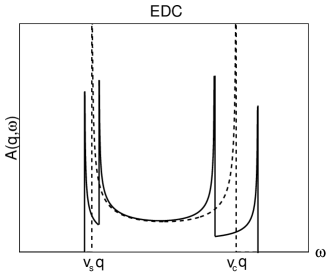
FIG. 1.: Energy distribution curve (EDC) of the spectral function $A(q,\omega)$ for a given $q\equiv k-k_{F}>0$. The solid (dashed) curve corresponds to the finite (zero) field case.

We first consider the Luttinger model with only $g_{4\perp}\neq 0$, which corresponds to the one-branch Luttinger model where there is no communication between right and left movers but still is spin-charge separated with corresponding velocities $v_{c,s}=v_{F}\pm g_{4\perp}/{2\pi}$. Although this is a simplified model it captures the basic physics of the electron decay into charge and spin collective excitations. (For zero field case see [4].) We restrict our attention to the $r=+$ branch, and to the electron injection process:

$$A(q,\omega)\sim\sum_{\sigma}\int_{\sigma h/v_{s}}^{q}dk_{s}\frac{\delta(\omega-\varepsilon_{c}(q-k_{s})-\varepsilon_{s}(k_{s})+\sigma h)}{|\varepsilon_{c}(q-k_{s})|^{\beta_{c}^{\sigma}}|\varepsilon_{s}(k_{s})-\sigma h|^{\beta_{s}^{\sigma}}},$$ (22)

At $h=0$ the spectral function has a continuum with well defined edges and power law singularities (Fig.1). The edges trace out the spin and charge dispersion relation, $\varepsilon_{c,s}(q)\equiv v_{c,s}k$. The lower (spinon) edge corresponds to where all the electron momentum is carried by the spinon and the upper (holon) edge where the anti-holon carries all q.

When $h\neq 0$ the region of nonzero spectral weight is in between the frequencies $v_{s}(k-k_{F\uparrow})<\omega<v_{c}(k-k_{F\downarrow})$ $(v_{c}>v_{s})$. We assume a small $\Delta v_{F}$ and keep the exponents of both singularities close to $1/2$. The spin and charge edges are respectively split by

$$\Delta\omega_{s} = 2h$$ (24)

$$\Delta\omega_{c} = 2\frac{v_{c}}{v_{s}}h\;\;.$$ (25)

The resulting energy distribution curve (EDC) is shown in Fig. 1. That the holon peak is also split by a magnetic field, while surprising at the first sight, can be understood as follows: As a holon is knocked out it is always accompanied by a spinon whose energy is shifted. What is not obvious is that the holon peak is split by a magnitude different from that of the splitting of the spinon peak. This is due to the fact that the splitting by the magnetic field takes place in $k-$space: The magnetic field splits the “spinon Fermi surface” by $\Delta k_{s,\sigma}=\sigma h/v_{s}$, without changing the “holon Fermi surface”. Since the single-electron Green’s function is a convolution of the spinon and holon Green’s functions, the energy change for the spinon peak is then $v_{s}\Delta k_{s,\sigma}$, while that for the holon peak is $v_{c}\Delta k_{s,\sigma}$.

The field effect on the momentum distribution curve (MDC) is very different. When the reference point of the spinon momentum changes, both edges respond equally in the MDC. As a result, both peaks are split by the same amount $2h/v_{s}$, as illustrated in Fig. 2.

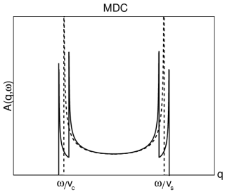
FIG. 2.: Momentum distribution curve (MDC) of the spectral function for a given $\omega\equiv E-E_{F}>0$. The solid (dashed) curve corresponds to the finite (zero) field result.

The difference in the splitting of the spinon and holon edges in the EDC provides a means to determine the spin quantum number of the two excitations. Suppose we divide the Zeeman energy between the holon and spinon in a parametrized fashion, i.e. $(1-\lambda)h$ for the spinon and $\lambda h$ for the anti-holon with $\lambda\in[0,1]$, from (22) we have

$$\frac{\Delta\omega_{c}}{\Delta\omega_{s}} = \frac{v_{c}}{v_{s}}$$ (26)

$$\Delta\omega_{c}-\Delta\omega_{s} = 2(\frac{v_{c}}{v_{s}}-1)(1-\lambda+\frac{v_{s}}{v_{c}}\lambda)h\;\;.$$ (27)

That tells us that if the edge splittings (24) and (25) are observed then $\lambda=0$ and all the magnetic coupling is carried by the spinon.

Let’s now turn to more realistic models. A finite $\gamma_{c}$ couples left to right movers and this introduces anomalous fermion exponents for the edge singularities and generates spectral weight in Fig. 1 for frequencies above the $v_{c}q$ edge and a small cusp below $-\varepsilon_{c}(q)$ [4]. The calculation of the spectral function in this case is rather involved but the power law behavior at the spinon and holon edges can be extracted easily by power counting:

$$A_{\sigma}(q,\omega\sim\varepsilon_{s}(q)) \sim |\omega-\varepsilon_{s}(q)+\sigma h|^{-\alpha_{s}^{\sigma}}$$ (28)

$$A_{\sigma}(q,\omega\sim\varepsilon_{c}(q)) \sim |\omega-\varepsilon_{c}(q)+\frac{v_{c}}{v_{s}}\sigma h|^{-\alpha_{c}^{\sigma}}$$ (29)

Where $\alpha_{s}^{\sigma}=\beta_{c}^{\sigma}-2\gamma^{\sigma}_{c}-\gamma^{\sigma}_{s}$, $\alpha_{c}^{\sigma}=\beta_{s}^{\sigma}-2\gamma^{\sigma}_{s}-\gamma^{\sigma}_{c}$, with $\gamma^{\sigma}_{\nu}=2\beta_{c}^{\sigma}\gamma_{\nu}$. The peak structure for both EDC at $q\neq 0$ and MDC at $\omega\neq 0$ remains essentially unchanged from Figs. 1 and 2.

Consider now the EDC at the Fermi momentum $k=k_{F}$. For the zero field case it has a power law singularity determined by the anomalous exponent $\gamma_{c}$ and no sign of spin-charge separation can be seen. Turning on a finite $h$ now splits this peak into four peaks, as seen in Fig. 3. Here even at $k_{F}$ and fairly strong coupling ($\gamma_{c}=0.2$, $\gamma_{s}\sim 0$) the sign of spin-charge separation is still visible as the Zeeman lines are split into contributions coming from the spinon and holon edges. As $\gamma_{c}$ increases we enter the strong coupling regime and the edge singularities are more and more obscured as the anomalous exponent dominates over the spin-charge separated character of the single particle spectrum.

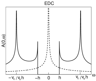
FIG. 3.: EDC at $k=k_{F}$ for $\gamma_{c}=0.2$ and $\gamma_{s}\sim 0$ (dash curve for $h=0$).

This splitting of one peak at Fermi momentum into four represents the most dramatic and direct manifestation of electron fractionalization. It unambiguously shows that the initial electron peak is in fact a composite of two different elementary excitations.

We turn next to MDC at the Fermi energy $E_{F}$. In the $h=0$ case it is, for $\gamma_{c}=0$, just the delta function $\delta(q)$. For $h\neq 0$ it is easy to verify, from the Lehmann representation of $A(q,\omega)$ and the properties of $\Psi_{r,\sigma}(x)$ zero modes in a magnetic field, that

$$A(q,0)\sim\sum_{\sigma}\delta(q-\sigma\frac{h}{v_{s}})\;.$$ (30)

The only interaction effect that remains in this MDC is the renormalization of $v_{F}$ to $v_{s}$ in the Zeeman splitting of the Fermi momentum. (A finite $\gamma_{c}$ would turn each delta function into a peak whose width and height depend on temperature in a power-law fashion.)

We stress that the contrasting behavior of the Zeeman-splittings in EDC and MDC reflects a generic feature of spin-charge separation. Namely, the main effect of the magnetic field is to split the spinon Fermi momentum.

Finally, the integrated spectral weight $N(\omega)\sim|\omega|^{\alpha}$, with $\alpha=2(\gamma^{\sigma}_{c}+\gamma^{\sigma}_{s})$. Here aside from the exponents the magnetic field has no other effect.

In several quasi-one-dimensoinal materials, ARPES experiments have seen two dispersive peaks[11, 12]. One interpretation is that these two peaks correspond to dispersing spinon and holon modes respectively. In the high $T_{c}$ cuprates, with fastly improving resolution in both energy and momentum, ARPES is now providing both EDC and MDC[13]. The theoretical interpretation of the lineshapes is actively being pursued[14]. Our results imply that studying the Zeeman effect on the spectral functions can provide valuable information about the quantum numbers of the elementary excitations.

We conclude with a few remarks concerning the experimental implementations. The Zeeman effects can in principle be studied using ARPES in a magnetic field. For 1D systems, an alternative technique to study the magnetic field effect is the momentum-resolved tunneling[16, 17]. We illustrate the quantitative effects of the magnetic field on the exponents by using seminconductor quantum wires as an example. We take[18] $K_{c}\approx 0.7$ and $E_{F}\approx 20meV$. For a vanishing field, $\alpha_{s}^{\sigma}\approx 0.47$ and $\alpha_{c}^{\sigma}\approx 0.48$. For a field of, say, $10$ T, and using $g\approx 0.4$ for GaAs, we estimate the corrections to $\alpha_{s}^{\sigma}$ and $\alpha_{c}^{\sigma}$ to be small, of the order of $\pm 0.05$. The experiments have to be done at temperatures below the Zeeman splitting, which are relatively easy to access. We also note that the situation would be even better for materials with high $g$ factors, such as InSb for which $g\sim-50$ [15].

We would like to thank G. Aeppli, N. Andrei, P.-A. Bares, S. A. Grigera, A. J. Schofield, and especially R. Gatt, for useful discussions. This work has been supported by the Robert A. Welch Foundation, NSF Grant NSF Grant No. DMR-0090071, and TCSUH.

REFERENCES

- [1] E.H. Lieb and F.Y. Wu, Phys. Rev. Lett. 20, 1445 (1968).
- [2] J. Voit, Rep. Prog. Phys. 58, 977 (1995).
- [3] For considerations based on spin transport, see Q. Si, Phys. Rev. Lett. 78, 1767 (1997); ibid. 81, 3191 (1998); Physica C341, 1519 (2000).
- [4] J. Voit, Phys. Rev. B 47, 6740 (1993); J. Phys.: Cond. Mat. 5,8305 (1993).
- [5] V. Meden and K.Schonhammer, Phys. Rev. B 46, 15753 (1992).
- [6] Y. Ren and P.W. Anderson, Phys. Rev. B 48, 16662 (1993).
- [7] J. von Delft and H. Schoeller, Ann. der Phys. 4, 225 (1998). For earlier discussions on the Klein factors, see G. Kotliar and Q. Si, Phys. Rev. B53, 12373 (1996).
- [8] H. Frahm and V.E. Korepin, Phys. Rev. B 43, 5653 (1991).
- [9] K. Penc and J. Solyom, Phys. Rev. B 47, 6273 (1993).
- [10] S. Rabello and Q. Si, in preparation (2002).
- [11] C. Kim et al, Phys. Rev. Lett. 77, 4054 (1996); J.D. Delinger et al, ibid. 82, 2540 (1999); P. Segovia et al., Nature 402, 504 (1999).
- [12] M. Grioni and J. Voit, J. de Phys. IV (Proceedings) 10, 91 (2000).
- [13] T. Valla et al., Science 285, 2110 (1999); P. V. Bogdanov et al., Phys. Rev. Lett. 85, 2581 (2001); A. Kaminski et al., ibid. 86, 1070 (2001).
- [14] E. Abrahams and C. M. Varma, Proc. Natl. Acad. Sci. USA 97, 5714 (2000); D. Orgad et al., Phys. Rev. Lett. 86, 4362 (2001); R. B. Laughlin, ibid. 79, 1726 (1997); P. W. Anderson, in High Temperature Superconductivity, eds. K. S. Bedell et al. (Addison-Wesley, Redwood City, 1990).
- [15] Crystal and Solid State Physics, eds. O. Madelung et al., Landolt-Bornstein, New Series, Group III, Vol. 16, Pt. a (Springer, Berlin, 1982).
- [16] S. Rabello et al., in preparation (2002).
- [17] A. Altland et al., Phys. Rev. Lett. 83, 1203 (1999).
- [18] O. M. Auslaender et al., Phys. Rev. Lett. 84, 1764 (2000).