Gorkov equations for a pseudo-gapped high temperature superconductor

Abstract

A theory of superconductivity based on the two-body Cooperon propagator is presented. This theory takes the form of a modified Gorkov equation for the Green’s function and allows one to model the effect of local superconducting correlations and long range phase fluctuations on the spectral properties of high temperature superconductors, both above and below $T_{c}$. A model is proposed for the Cooperon propagator, which provides a simple physical picture of the pseudo-gap phenomenon, as well as new insights into the doping dependence of the spectral properties. Numerical calculations of the density of states and spectral functions based on this model are also presented, and compared with the experimental STM and ARPES data. It is found, in particular, that the sharpness of the peaks in the density of states is related to the strength and the range of the superconducting correlations and that the apparent pseudo-gap in STM and ARPES can be different, although the underlying model is the same.

I Introduction

The anomalous properties of high temperature superconductors (HTS) have been the object of many investigations over the last ten years.[2] Among these anomalous properties, the pseudo-gap phenomenon (a substantial decrease of the one particle density of states near the Fermi energy in the normal state below a certain temperature $T^{*}$) has been studied by several experimental techniques. In tunneling spectroscopy experiments, in particular, the pseudo-gap manifests itself as a gap in the excitation spectrum.[3] On the theoretical front, many competing models have been proposed.[4, 5, 6, 7, 8, 9, 10, 11, 12, 13] One of the popular interpretations of the pseudo-gap is that superconductivity forms locally at $T^{*}$, but the phases of distant superconducting “droplets” remain incoherent until the superconducting transition temperature $T_{c}$ is reached.[4, 5] This view is supported by an increasing evidence that the pseudo-gap phenomenon is intimately connected to the underlying superconducting phase, mainly because the $d$-wave symmetry of the pseudo-gap is the same as that of the gap in the superconducting phase.[14, 15] The phase fluctuation model of the pseudo-gap state is different from the usual theory of superconducting fluctuations, because the latter is only valid near $T_{c}$, and involves both size and phase fluctuations.[16]

A theory of the pseudo-gap above $T_{c}$ has also consequences below $T_{c}$. In particular, it is connected to the character of the excitations responsible for destroying superconductivity. Different mechanisms (thermal phase fluctuations, quantum phase fluctuations, nodal quasiparticles) may all contribute to the properties in the superconducting state, and these contributions may be of varying importance if one considers low temperatures or temperatures near $T_{c}$.[17] One may add that the clue to a theory of high temperature superconductivity will go through the explanation of detailed properties, like the absence of quasiparticles above $T_{c}$ and their appearance below $T_{c}$,[18] or the anomalous properties of the density of states in vortices.[19]

Within the BCS theory, the inclusion of phase fluctuations in a droplet model must be done in two steps. First, one introduces a local BCS gap, with a phase, and then one must somehow analyze the phase fluctuations in a second analytical step distinct from the first. The theory of Franz and Millis[20] gives an example of this type of approach. Starting from the form of the Green’s function in a uniform superflow, they extend it semi-classically to non-uniform situations assuming slow spatial variations of the superfluid velocity. This Green’s function is then averaged over a Gaussian distribution of velocity fluctuations, which relates the result to a correlation function of the velocities. A similar approach has been used by Kwon and Dorsey,[21] who treat the coupling to the fluctuating phase using a self-consistent perturbation theory. As emphasized by Geshkenbein et al.[12] and Randeria,[22] strong pairing correlations should however be incorporated at the basis of any model of the pseudo-gap regime.

A systematic theory of the effect of phase fluctuations on the density of states (and other properties) in HTS, above and below $T_{c}$, must start by putting the phase-phase correlation function at the core of the theory for superconductivity, at the same level as the size of the local gap. This program implies that one avoids developing the theory of superconductivity by defining a gap function and an anomalous propagator. This is equivalent to writing the BCS theory in a particle number conserving scheme (i.e. in the canonical ensemble, avoiding the definition of an anomalous amplitude between states with different particle numbers). This theory has actually been written down forty years ago by Kadanoff and Martin[23] (KM), and rediscovered by others, in particular for the discussion of Josephson arrays.[24] The KM theory is based on the two-body Cooperon propagator, and describes quite naturally the effect of phase fluctuations. This theory has already been applied to the HTS in a nice series of papers by Levin et al.,[25] but with a different interpretation (not related to phase fluctuations), a different focus, and a different formalism than in our work. In this paper we rewrite the basic KM equations for the case of a lattice Hamiltonian, we show again how the standard BCS theory is recovered with a straightforward approximation for the two-body Cooperon correlation function, and we then derive the basic equations for a pseudo-gap state, in particular the equivalent Gorkov equations which have to be used in the calculation of vortex states.

II Kadanoff-Martin equations in a lattice model

We consider the lattice Hamiltonian

$${\cal H}=\sum_{ij\sigma}t_{ij}\,c^{\dagger}_{i\sigma}c_{j\sigma}+\sum_{ij}V_{ij}\,b^{\dagger}_{i}b_{j}.$$ (1)

In this, $c^{\dagger}_{i\sigma}$ creates an electron at site $i$ and $b^{\dagger}_{i}=c^{\dagger}_{i\downarrow}c^{\dagger}_{i\uparrow}$ creates a Cooper pair at site $i$. We assume that $t$ and $V$ are symmetric and real. The usual Gorkov equations can then be written as a single equation:

$$\big{[}{\cal G}^{0}(\omega_{n})\big{]}^{-1}{\cal G}(\omega_{n})=\openone+\tilde{\Sigma}(\omega_{n})\,{\cal G}(\omega_{n}),$$ (2)

where ${\cal G}_{ij}(\tau)=-\langle T_{\tau}\{c_{i\uparrow}(\tau)c^{\dagger}_{j\uparrow}(0)\}\rangle$ and

$$\tilde{\Sigma}_{ij}(\omega_{n})=-\sum_{r_{1}r_{2}}V_{ir_{1}}B_{r_{1}}B^{\star}_{r_{2}}V_{r_{2}j}{\cal G}_{ji}^{0}(-\omega_{n}).$$ (3)

$\big{[}{\cal G}^{0}(\omega_{n})\big{]}^{-1}_{ij}=i\omega_{n}\delta_{ij}-t_{ij}$ is the free Green’s function, $\omega_{n}$ are the odd Matsubara frequencies, and $B_{\ell}=\left\langle b_{\ell}\right\rangle$. The notation $\big{[}{\cal G}^{0}\big{]}^{-1}{\cal G}$ implies matrix multiplication in the $\{i,\,j\}$ space. These equations are supplemented by the self-consistent equation for $B_{i}$ (or $\Delta_{i}$) and the self-consistent equation relating the number of particles $N$ to the chemical potential. The equation for $B_{i}$ is

$$B_{i}=-{\cal F}_{ii}(0^{+})=-\frac{1}{\beta}\sum_{\omega_{n}}{\cal F}_{ii}(\omega_{n})\,e^{-i\omega_{n}0^{+}}$$ (4)

with ${\cal F}^{\star}_{ij}(\tau)=-\langle T_{\tau}\{c^{\dagger}_{i\downarrow}(\tau)c^{\dagger}_{j\uparrow}(0)\}\rangle$.

The Kadanoff-Martin correlation function description of superconductivity consists simply (after a long and thorough discussion of higher order correlation functions) in replacing $\tilde{\Sigma}$ in Eq. (2) by

$$\Sigma_{ij}(\omega_{n})=-\frac{1}{\beta}\sum_{\omega_{m}}\sum_{r_{1}r_{2}}V_{ir_{1}}L_{r_{2}r_{1}}(\omega_{n}+\omega_{m})V_{r_{2}j}{\cal G}_{ji}^{0}(\omega_{m})$$ (5)

where $L_{r_{2}r_{1}}(\tau)=\left\langle T_{\tau}\left\{b_{r_{1}}(\tau)b^{\dagger}_{r_{2}}(0)\right\}\right\rangle$ is the Cooperon propagator. The self-consistent equation for $B$ is replaced by the equations

$$L_{r_{2}r_{1}}(\Omega_{m})=-\frac{1}{\beta}\sum_{\omega_{n}}{\cal G}_{r_{2}r_{1}}(\Omega_{m}+\omega_{n}){\cal G}^{0}_{r_{1}r_{2}}(-\omega_{n})$$ (8)

$$\quad-\frac{1}{\beta}\sum_{\omega_{n}}\sum_{ij}{\cal G}_{ir_{2}}(\Omega_{m}+\omega_{n}){\cal G}^{0}_{ir_{2}}(-\omega_{n})V_{ji}L_{jr_{1}}(\Omega_{m})$$

for $T>T_{c}$, and

$$L_{r_{2}r_{1}}(\Omega_{m})=$$ (9)

$$\quad-\frac{1}{\beta}\sum_{\omega_{n}}\sum_{ij}{\cal G}_{ir_{2}}(\Omega_{m}+\omega_{n}){\cal G}^{0}_{ir_{2}}(-\omega_{n})V_{ji}L_{jr_{1}}(\Omega_{m})$$ (10)

for $T<T_{c}$, where $\Omega_{m}$ are the even Matsubara frequencies. The fact that the inhomogeneous term in the ladder equation for $L$ has to be dropped when calculating the order parameter in the condensed state is not much commented upon in the original paper of KM, but it is related to the range of $L_{r_{2}r_{1}}(\Omega_{m})$, which is finite above $T_{c}$ and infinite below $T_{c}$ (see below). In fact, the quantity $\sum_{r_{1}r_{2}}L_{r_{2}r_{1}}(\Omega_{m})$ is of the order $N^{2}$ below $T_{c}$ (where $N$ is the number of sites) whereas the corresponding sum of the inhomogeneous term in Eq. (8) is only of order $N$. The usual BCS theory is recovered by setting

$\displaystyle L_{r_{2}r_{1}}(\tau)=B_{r_{1}}B^{\star}_{r_{2}},\quad L_{r_{2}r_{1}}(\Omega_{m})=\beta B_{r_{1}}B^{\star}_{r_{2}}\delta_{\Omega_{m},0}$

in Eq. (5). The self-consistent equation Eq. (9) for $L$ then goes over into the self-consistent equation Eq. (4) for $B$, and clearly Eq. (5) goes into Eq. (3). In the BCS framework, the Thouless criterion for $T_{c}$ becomes the gap equation for $T<T_{c}$.

The KM description of superconductivity, which is entirely based on the properties of the function $L$, is thus seen to be a natural starting point if one wants to introduce explicitly local order and phase fluctuations in the physical description of high temperature superconductors. This is done in the next section.

III Phenomenological description of a pseudo-gapped superconductor

Our fundamental assumption is that Eq. (5) is generally valid, in the sense that it expresses in general the single particle Green’s function in terms of the Cooperon propagator, regardless of the model or the approximations involved in calculating this propagator. Our purpose in this paper is to explore the experimental consequences of a simple heuristic form for $L$, which is the translation of the physical picture presented in the Introduction. For $T>T_{c}$, we write:

$$L_{r_{2}r_{1}}(\tau)=|B^{0}|^{2}\,R(r_{12}/\varrho_{0})+|B^{1}|^{2}\,F(r_{2}-r_{1},\,\tau)$$ (12)

with $r_{12}=|r_{2}-r_{1}|$ and $R(x)$ some cutoff function which vanishes rapidly for $x>1$. This equation expresses the fact that there are strong superconducting correlations at the scale $\varrho_{0}$, represented by a finite value of $B^{0}$, going to zero gradually at a temperature $T^{*}$. The strength of the superconducting correlations between “droplets” is represented by an amplitude $B^{1}$ and some function $F$ describing essentially the correlations in an $XY$ model above the Kosterlitz-Thouless (KT) transition. Both $B^{1}$ and $F$ will be temperature dependent. As $T$ approaches $T_{c}$ from above (we identify $T_{c}$ with the KT transition temperature), the correlation length of $F$ diverges and $F$ approaches 1. For $T<T_{c}$, we write:

$$L_{r_{2}r_{1}}(\tau)=|B^{0}|^{2}\,R(r_{12}/\varrho_{0})+B^{1}_{r_{1}}{B^{1}_{r_{2}}}^{\star},$$ (13)

where only the amplitude $B^{1}$ carries a phase. The assumption here is that short range correlations have a strong incoherent part, even in the superconducting state. When introduced into the equation for the self-energy, Eq. (13) for $L$ means that the self-energy in the superconducting state is the sum of a coherent and an incoherent part; this appears to be the case in some recent calculations based on a fermion-boson model.[26] Inspection of Eqs. (13) and (5) shows that if, in the ladder approximation for a homogeneous system, it turns out that $L_{r_{2}r_{1}}$ is the sum of a constant term and a term of finite range, then the constant term will obey Eq. (9), whereas the finite range term will obey Eq. (8).

Eqs. (III) translate into the following equation for ${\cal G}$:

$$\big{[}\tilde{\cal G}^{0}(\omega_{n})\big{]}^{-1}{\cal G}(\omega_{n})=\openone+\Sigma^{1}(\omega_{n})\,{\cal G}(\omega_{n}),$$ (14)

where

$$\big{[}\tilde{\cal G}^{0}(\omega_{n})\big{]}^{-1}_{ij}=\big{[}{\cal G}^{0}(\omega_{n})\big{]}^{-1}_{ij}$$ (15)

$$\qquad+\sum_{r_{1}r_{2}}V_{ir_{1}}|B^{0}|^{2}\,R(r_{12}/\varrho_{0})\,V_{r_{2}j}{\cal G}^{0}_{ji}(-\omega_{n})$$ (16)

and

$$\Sigma^{1}_{ij}(\omega_{n}) = -\frac{1}{\beta}\sum_{\omega_{m}}\sum_{r_{1}r_{2}}V_{ir_{1}}|B^{1}|^{2}F(r_{2}-r_{1},\,\omega_{n}+\omega_{m})$$ (19)

$$\hskip 72.00008pt\times V_{r_{2}j}{\cal G}^{0}_{ji}(\omega_{m}),\;T\!>\!T_{c}$$

$$\Sigma^{1}_{ij}(\omega_{n}) = {\displaystyle-\!\!\sum_{r_{1}r_{2}}V_{ir_{1}}B^{1}_{r_{1}}{B^{1}_{r_{2}}}^{\!\star}V_{r_{2}j}{\cal G}^{0}_{ji}(-\omega_{n})},\;T\!<\!T_{c}.$$ (20)

Inspection of Eq. (20), together with Eq. (14), shows that below $T_{c}$, a pseudo-gapped superconductor obeys the following modified Gorkov equations:

$$\left\{\big{[}\tilde{\cal G}^{0}(\omega_{n})\big{]}^{-1}{\cal G}(\omega_{n})\right\}_{\!ij}+\!\sum_{\ell}V_{i\ell}B_{\ell}^{1}\tilde{\cal F}_{ij}^{\star}(\omega_{n}) = \delta_{ij}$$ (22)

$$\left\{\big{[}{\cal G}^{0}(-\omega_{n})\big{]}^{-1}\!\tilde{\cal F}^{\star}(\omega_{n})\right\}_{\!ij}\!\!-\!\sum_{\ell}V_{\ell i}{B_{\ell}^{1}}^{\star}{\cal G}_{ij}(\omega_{n}) = 0.$$ (23)

Quantum Monte Carlo (QMC) calculations of the pairing correlations were recently reported for the attractive Hubbard model at zero temperature.[27] Although these results are restricted to short distances ($\sim$ 6–10 lattice sites) we tentatively connect our model to the QMC calculations with the following arguments. For the system sizes considered in the QMC calculations (typically $14\times 14$ sites) the correlation function for the largest distance in the system has not converged to its asymptotic value. We attribute the slow decrease of the correlations at intermediate distances (see inset of Fig. 4 in Ref. [27]) to a large value of $\varrho_{0}$ with respect to the system size. The results of Ref. [27] also show that the strength of the pairing correlations at intermediate distances increases, and differs increasingly from the BCS result, as the Hubbard interaction $U/t$ increases. Closer inspection of the data in Fig. 3 of Ref. [27] indicates that the ratio of the BCS to the QMC correlations at intermediate distances is also an increasing function of $U/t$. The simplest BCS approximation to Eq. (13) is to replace the cutoff function $R$ by $1$, describing correlations which are independent of $r_{1}$ and $r_{2}$ (in a homogeneous system, the second term of Eq. (13) is a constant $|B^{1}|^{2}$). With this approximation, one can account for the above trends by assuming that both $B^{0}$ and the ratio $B^{0}/B^{1}$ increase as $U/t$ increases. Finally, we shall include in our numerical calculations the “onsite” correlations found in Ref. [27] for distances within two lattice spacings, by adding a term

$$L^{\text{os}}_{r_{2}r_{1}}=\left(|B^{0}|^{2}+|B^{1}|^{2}\right)e^{-2\,r_{12}/a}$$ (24)

to the model Eqs. (III), where $a$ is the lattice parameter. We find, however, that this correction has a negligible impact on the spectral functions, and could equally be dropped without changing the results presented below.

IV Numerical results

We now use the general equations derived in Section II, together with the model Eqs. (III) and (24), to calculate the temperature dependence of the density of states and spectral functions in a homogeneous system. The calculations are compared with the STM and ARPES experimental results for BSCCO. In order to reduce the number of adjustable parameters, we take for the correlation function $F(\mathchoice{{\hbox{\boldmath$\displaystyle r$}}}{{\hbox{\boldmath$\textstyle r$}}}{{\hbox{\boldmath$\scriptstyle r$}}}{{\hbox{\boldmath$\scriptscriptstyle r$}}},\,\tau)=\exp[-r/\xi(T)]$, which describes time-independent phase-phase correlations above $T_{c}$. The correlation length $\xi$ is equal to $\varrho_{1}\alpha\exp[b/\sqrt{(T-T_{c})/J}]$, with $\alpha\approx 0.21$, $b\approx 1.73$, and $J\approx T_{c}/0.89$.[28] The length-scale $\varrho_{1}$ is the lattice parameter of the effective $2D-XY$ model describing phase fluctuations. We found that the main features in the spectral properties above $T_{c}$ are rather insensitive to the details of the correlation function. We have explicitly checked this point by comparing different functions $F$, in particular functions which give a better description of the correlations in the $XY$ model. The cutoff function $R$ is modeled as $\exp(-r/\varrho_{0})$.

The four parameters $\varrho_{0}$, $\varrho_{1}$, $B^{0}$, and $B^{1}$ are chosen to achieve good agreement with the experimental results. We use the value $\varrho_{0}=50a$; if the first term in the right-hand side of Eq. (13) is the dominant one ($B^{0}>B^{1}$), we found that a relatively large value of $\varrho_{0}$ is needed in order to obtain well developed coherence peaks in the zero temperature density of states. In addition, we see that, according to the previous discussion, $\varrho_{0}$ must be large with respect to $\sim 14a$. The parameter $\varrho_{1}$ controls the temperature evolution of the spectral functions above $T_{c}$, and takes the value $\varrho_{1}=5a$. The larger $\varrho_{1}$, the wider the temperature region above $T_{c}$ in which finite range phase coherence contributes to the pseudo-gap. The amplitude $B^{0}$ is adjusted to fix the gap energy to $\sim 40$ meV. Finally, the ratio $B^{0}/B^{1}$ is varied in order to control the relative importance of short range superconducting correlations and long-range phase fluctuations. The behavior of the resulting Cooperon propagator $L(\mathchoice{{\hbox{\boldmath$\displaystyle r$}}}{{\hbox{\boldmath$\textstyle r$}}}{{\hbox{\boldmath$\scriptstyle r$}}}{{\hbox{\boldmath$\scriptscriptstyle r$}}})$ is illustrated in Fig. 1 for temperatures below and above $T_{c}$ and for different values of $|B^{0}/B^{1}|$.

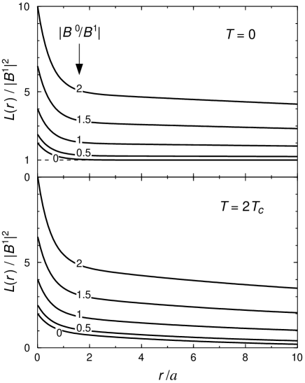
FIG. 1.: Model two-body Cooperon correlation function at temperatures below and above $T_{c}$. The increase of the correlations for $r\lesssim a$ is due to $L^{\text{os}}$ given in Eq. (24). Below $T_{c}$, $L(r)$ converges to the finite asymptotic value $|B^{1}|^{2}$ at distances of the order $\varrho_{0}$ if $B^{0}>0$ and of the order $a$ if $B^{0}=0$. Above $T_{c}$, the range of $L(r)$ is finite. If $B^{0}>0$, this range is given by $\max(\varrho_{0},\,\xi(T))$ while if $B^{0}$ vanishes it is given by $\xi(T)$.

For a translationally invariant system and our model Cooperon propagator, Eq. (5) can be recast as

$$\Sigma(\mathchoice{{\hbox{\boldmath$\displaystyle k$}}}{{\hbox{\boldmath$\textstyle k$}}}{{\hbox{\boldmath$\scriptstyle k$}}}{{\hbox{\boldmath$\scriptscriptstyle k$}}},\,\omega_{n})=\frac{1}{(2\pi)^{2}}\int_{\text{BZ}}\frac{V^{2}(\mathchoice{{\hbox{\boldmath$\displaystyle q$}}}{{\hbox{\boldmath$\textstyle q$}}}{{\hbox{\boldmath$\scriptstyle q$}}}{{\hbox{\boldmath$\scriptscriptstyle q$}}})L(\mathchoice{{\hbox{\boldmath$\displaystyle q$}}}{{\hbox{\boldmath$\textstyle q$}}}{{\hbox{\boldmath$\scriptstyle q$}}}{{\hbox{\boldmath$\scriptscriptstyle q$}}})d\mathchoice{{\hbox{\boldmath$\displaystyle q$}}}{{\hbox{\boldmath$\textstyle q$}}}{{\hbox{\boldmath$\scriptstyle q$}}}{{\hbox{\boldmath$\scriptscriptstyle q$}}}}{i\omega_{n}+\varepsilon_{\mathchoice{{\hbox{\boldmath$\displaystyle q$}}}{{\hbox{\boldmath$\textstyle q$}}}{{\hbox{\boldmath$\scriptstyle q$}}}{{\hbox{\boldmath$\scriptscriptstyle q$}}}-\mathchoice{{\hbox{\boldmath$\displaystyle k$}}}{{\hbox{\boldmath$\textstyle k$}}}{{\hbox{\boldmath$\scriptstyle k$}}}{{\hbox{\boldmath$\scriptscriptstyle k$}}}}}$$ (25)

where $V(\mathchoice{{\hbox{\boldmath$\displaystyle q$}}}{{\hbox{\boldmath$\textstyle q$}}}{{\hbox{\boldmath$\scriptstyle q$}}}{{\hbox{\boldmath$\scriptscriptstyle q$}}})=V_{0}+2V_{1}(\cos q_{x}a+\cos q_{y}a)$, $L(\mathchoice{{\hbox{\boldmath$\displaystyle q$}}}{{\hbox{\boldmath$\textstyle q$}}}{{\hbox{\boldmath$\scriptstyle q$}}}{{\hbox{\boldmath$\scriptscriptstyle q$}}})$ is the Fourier transform of $L(\mathchoice{{\hbox{\boldmath$\displaystyle r$}}}{{\hbox{\boldmath$\textstyle r$}}}{{\hbox{\boldmath$\scriptstyle r$}}}{{\hbox{\boldmath$\scriptscriptstyle r$}}})$, and $\varepsilon_{\mathchoice{{\hbox{\boldmath$\displaystyle k$}}}{{\hbox{\boldmath$\textstyle k$}}}{{\hbox{\boldmath$\scriptstyle k$}}}{{\hbox{\boldmath$\scriptscriptstyle k$}}}}$ is the free dispersion. Here, $V_{0}$ and $V_{1}$ are the onsite and nearest-neighbor potentials, respectively, and we neglect next-nearest neighbor interactions; we assume $V_{1}=V_{0}/4$ in all of our calculations. For the dispersion, we use a tight-binding expression which fits the BSCCO Fermi surface and corresponds to a bandwidth of 2 eV.[29] The self-energy at real frequencies is evaluated by making the analytic continuation $i\omega_{n}\rightarrow\omega^{+}=\omega+i0^{+}$ in Eq. (25) and discretizing the BZ integral.[30] The spectral function is then calculated according to $A(\mathchoice{{\hbox{\boldmath$\displaystyle k$}}}{{\hbox{\boldmath$\textstyle k$}}}{{\hbox{\boldmath$\scriptstyle k$}}}{{\hbox{\boldmath$\scriptscriptstyle k$}}},\,\omega)=-\frac{1}{\pi}\text{Im}\big{\{}\!\left[\omega^{+}-\varepsilon_{\mathchoice{{\hbox{\boldmath$\displaystyle k$}}}{{\hbox{\boldmath$\textstyle k$}}}{{\hbox{\boldmath$\scriptstyle k$}}}{{\hbox{\boldmath$\scriptscriptstyle k$}}}}-\Sigma(\mathchoice{{\hbox{\boldmath$\displaystyle k$}}}{{\hbox{\boldmath$\textstyle k$}}}{{\hbox{\boldmath$\scriptstyle k$}}}{{\hbox{\boldmath$\scriptscriptstyle k$}}},\,\omega^{+})\right]^{-1}\!\big{\}}$, and the density of states is $N(\omega)\propto\int_{\text{BZ}}A(\mathchoice{{\hbox{\boldmath$\displaystyle k$}}}{{\hbox{\boldmath$\textstyle k$}}}{{\hbox{\boldmath$\scriptstyle k$}}}{{\hbox{\boldmath$\scriptscriptstyle k$}}},\,\omega)\,d\mathchoice{{\hbox{\boldmath$\displaystyle k$}}}{{\hbox{\boldmath$\textstyle k$}}}{{\hbox{\boldmath$\scriptstyle k$}}}{{\hbox{\boldmath$\scriptscriptstyle k$}}}$. It is easy to check from Eq. (25) that, if $L(\mathchoice{{\hbox{\boldmath$\displaystyle q$}}}{{\hbox{\boldmath$\textstyle q$}}}{{\hbox{\boldmath$\scriptstyle q$}}}{{\hbox{\boldmath$\scriptscriptstyle q$}}})>0$ — a condition obeyed by our model — then the Green’s function is analytic in the upper half of the complex plane, the spectral function $A(\mathchoice{{\hbox{\boldmath$\displaystyle k$}}}{{\hbox{\boldmath$\textstyle k$}}}{{\hbox{\boldmath$\scriptstyle k$}}}{{\hbox{\boldmath$\scriptscriptstyle k$}}},\,\omega)$ is positive, and the Green’s function goes to zero as $\omega^{-1}$ for $|\omega|\rightarrow\infty$.

A Scanning tunneling spectroscopy

FIG. 2.: Tunneling conductance as a function of temperature. The model parameters represent (a) underdoped ($V_{0}B^{0}=15$ meV, $B^{0}/B^{1}=2$) and (b) overdoped ($V_{0}B^{0}=7$ meV, $B^{0}/B^{1}=0.5$) situations. The critical temperature is $T_{c}=80$ K (bold line). The dashed lines show the $T=300$ K spectra corresponding to $B^{1}=0$ and (a) $V_{0}B^{0}=7.5$ meV, (b) $V_{0}B^{0}=3.5$ meV. The curves have been shifted for clarity.

Neglecting possible anisotropies of the tunneling matrix element as well as $k_{z}$-dispersion effects, we calculate the tunneling conductance as the convolution of the density of states with the derivative of the Fermi function. The result is shown in Fig. 2 for various temperatures. In order to focus on the effect of local superconductivity and phase fluctuations, we have kept the model parameters independent of temperature: the whole temperature dependence of the curves, in Fig. 2, relates to the variation of the correlation length $\xi$ and Fermi function with $T$. A better fit to the experimental data could be obtained, in principle, by allowing the amplitudes $B^{0}$ and $B^{1}$ to vary with temperature. This would not, however, change the qualitative conclusions we wish to draw. In Fig. 2(a), $B^{0}$ is larger than $B^{1}$ while in Fig. 2(b) $B^{1}$ is larger than $B^{0}$. In the next section, we argue that these two typical cases correspond to underdoped (UD) and overdoped (OD) situations, respectively. The spectra shown in Fig. 2 reproduce some of the characteristic features observed experimentally in BSCCO samples.[3] Both UD and OD curves evolve smoothly across $T_{c}$ into a pseudo-gapped spectrum, the peak-to-peak distance remaining approximately temperature independent. Moreover, the coherence peaks and the gap structure disappear more rapidly in the OD case as the temperature is raised, which is also consistent with the experimental findings. The model, however, is not able to account for a number of experimental observations, such as the asymmetry in the temperature dependence of the positive and negative-bias conductance peaks, or the dip structure recorded at $\sim 2\Delta$ below $T_{c}$. We also note that the model Eqs. (III) has $s$-wave symmetry. The calculated spectra are therefore not expected to agree in details with experiment at low energies.

According to our model, the local superconducting correlations responsible for the high temperature pseudo-gap also have implications below $T_{c}$. In the underdoped case, the local (incoherent) superconducting correlations broaden the zero temperature density of states. The resulting conductance spectra have small coherence peaks and a rounded line-shape around the fermi energy. In the overdoped case, in contrast, the $T=0$ curve looks more like a ($s$-wave) BCS spectrum.

As the temperature increases from zero to $T_{c}$, the density of states remains unchanged in both UD and OD cases, and the temperature dependence of the conductance spectra relates solely to the Fermi function. This behavior persists above $T_{c}$ in the UD case owing to the dominant role of $B^{0}$ (which is $T$-independent in our calculations). In the OD situation, on the contrary, the gap fills in rapidly above $T_{c}$ as the contribution of $B^{1}$ disappears due to increasing phase fluctuations; at elevated temperatures, only a weak pseudo-gap due to $B^{0}$ remains. Fig. 2 also illustrates the effect of the temperature dependence of the amplitudes $B^{0}$ and $B^{1}$. At room temperature, $B^{1}$ is expected to vanish and $B^{0}$ is expected to be smaller than at low temperature. Taking $B^{1}=0$ and $B^{0}(300~{}{\text{K}})=B^{0}(0~{}{\text{K}})/2$, one obtains the dashed spectra in Fig. 2, which no longer exhibit a sizable pseudo-gap structure.

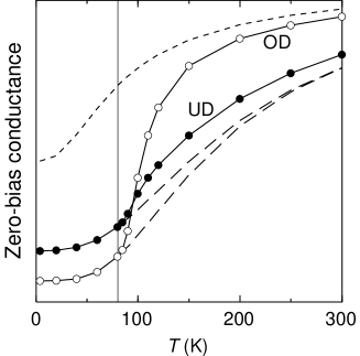
FIG. 3.: Calculated zero-bias conductance as a function of temperature for underdoped (UD, black symbols), and overdoped (OD, white symbols) systems. The parameters are the same as in Fig. 2. The dashed lines show the conductance obtained by thermally broadening the $T=0$ spectra. The dotted line is obtained by letting $B^{1}$ go to zero in the OD situation. The vertical axis starts at zero.

The difference between the temperature evolutions of the UD and OD spectra is best seen in Fig. 3, where we plot the calculated zero-bias conductance. Below $T_{c}$, the zero-bias conductance is larger in the UD case due to strong local correlations. Above $T_{c}$, the conductance increases sharply in the OD case, corresponding to the filling of the gap. In either UD and OD cases, the zero-bias conductance above $T_{c}$ is larger than the value expected by thermally broadening the $T=0$ spectra (see Fig. 3).

From a general point of view, one can confirm from our calculations that the sharpness of the peaks in the density of states (and correspondingly the size of the zero-bias conductance) is related to the strength and range of the superconducting correlations. The larger the ratio $B^{1}/B^{0}$ and/or the longer the range $\varrho_{0}$, the sharper the peaks (the smaller the zero-bias conductance). As an example, we show in Fig. 3 the conductance obtained by letting the coherence term $B^{1}$ go to zero in the OD situation. Comparison of the curves with and without $B^{1}$ shows that the phase coherence has the effect to depress the density of states at the Fermi energy — therefore raising the coherence peaks — below $T_{c}$ and in some temperature range above $T_{c}$, where the correlation length $\xi(T)$ is large.

B Angle-resolved photoemission

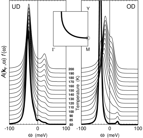
FIG. 4.: Calculated ARPES intensity near $(\pi,\,0)$ as a function of temperature for underdoped (UD) and overdoped (OD) systems. The parameters are the same as in Fig. 2. The curves have been shifted for clarity. Inset: representation of the Brillouin zone showing the Fermi surface used in the calculations and the Fermi crossing near $(\pi,\,0)$.

Experimentally, it is found that the temperature dependence of the energy dispersion curves measured by ARPES near $(\pi,\,0)$ depends on doping. In overdoped samples, the leading-edge midpoint energy moves toward the Fermi energy — suggesting that the gap closes — as $T$ increases above $T_{c}$. The temperature variations of the midpoint energy are usually smaller in underdoped samples.[31, 32]

Apart from a matrix element, the ARPES intensity is just the product of the spectral and Fermi functions. This quantity, calculated at the Fermi crossing near the $M$ point, is shown in Fig. 4 as a function of temperature. A clear difference between the temperature evolution of the spectral peak in the UD and OD cases can be seen. Consistently with experiment, the peak shifts toward the Fermi energy in the OD case as $T$ increases. In the UD case, the peak position is to first approximation independent of temperature. Below $T_{c}$, the curves are almost identical to the spectrum at $T_{c}$ (because the temperature $T<T_{c}\approx 7$ meV is small with respect to the peak energy $\sim 35$ meV) and are not shown. One can see that the quasiparticle peak is much sharper at $T_{c}$ in the overdoped as compared to the underdoped system. This has also been seen experimentally[32] and can easily be understood in our model. The destruction of long range order by phase fluctuations clearly affects qualitatively the spectral functions in the OD case where the transition across $T_{c}$ is accompanied by a decrease of the quasiparticle lifetime and increase of the intensity at the Fermi energy.

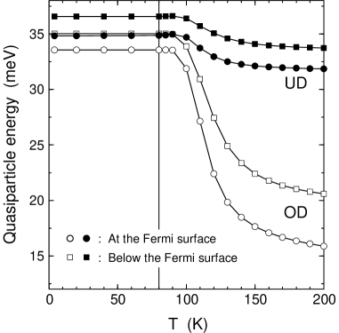
FIG. 5.: Temperature dependence of the quasiparticle energy (maximum of the curves in Fig. 4) at the Fermi crossing near $(\pi,\,0)$ for underdoped (UD, black circles), and overdoped (OD, white circles) systems. The squares show the energy of the quasiparticle at a $\textstyle k$ point just below the Fermi surface along the $M$–$Y$ line.

The position of the main quasiparticle peak in Fig. 4 is reported in Fig. 5 as a function of temperature. The temperature dependence of the gap was studied in Refs [20] and [32] by fitting the experimental ARPES curves to a three parameters Green’s function. For overdoped samples, the gap was found to decrease with increasing temperature (Ref. [32]), in a way very similar to what we obtain in the OD case, although the decrease was found to begin already below $T_{c}$. Note that a small finite gap persists at all temperatures in our calculations, since no temperature dependence of $B^{0}$ and $B^{1}$ was taken into account. In a real situation, $B^{0}$ and $B^{1}$ would both vanish at some temperature above $T_{c}$. In the underdoped samples, the gap was found to be temperature independent within error bars (Ref. [32]) or slightly decreasing above $T_{c}$ (Ref. [20]). The trend in Fig. 5 is similar. The slight decrease of the gap above $T_{c}$ in the UD case results from the suppression of the phase correlations as the temperature is raised.

The spectral line-shapes in Fig. 4 are considerably sharper than what is usually measured by ARPES, especially at elevated temperatures. The estimated experimental resolution of $\sim 10$ meV cannot alone explain this difference. Similar conclusions have been reached in Ref. [20]. It was shown there that the inverse quasiparticle lifetime implied by fitting the experimental spectra are an order of magnitude larger in ARPES with respect to STM. Inhomogeneities in the sample properties could explain this discrepancy,[33] since a much larger region of the sample surface is probed by ARPES compared to STM.

The temperature dependence of the OD quasiparticle peak in Fig. 5 contrasts with the apparent temperature independence of the gap width in Fig. 2. The coherence peaks in the density of states are due to quasiparticle states with momenta just nearby $\mathchoice{{\hbox{\boldmath$\displaystyle k$}}}{{\hbox{\boldmath$\textstyle k$}}}{{\hbox{\boldmath$\scriptstyle k$}}}{{\hbox{\boldmath$\scriptscriptstyle k$}}}_{\text{F}}$. Therefore, one may expect that the energies of all these quasiparticles evolve in the same way as the temperature increases. In this case, the coherence peaks would rigidly follow this temperature evolution and both the STM and ARPES gaps would close in the OD situation. We have found, however, that in our model the energies of the quasiparticles at and nearby $\mathchoice{{\hbox{\boldmath$\displaystyle k$}}}{{\hbox{\boldmath$\textstyle k$}}}{{\hbox{\boldmath$\scriptstyle k$}}}{{\hbox{\boldmath$\scriptscriptstyle k$}}}_{\text{F}}$ have different temperature dependencies in the OD case. This is illustrated in Fig. 5, where we plot the energy of a quasiparticle with a momentum $\textstyle k$ just below the Fermi surface along the $M$–$Y$ line. For $T<T_{c}$, this particular $\textstyle k$ point contributes to the coherence peaks in the density of states, since the corresponding energy is within $\sim 2$ meV of the energy at $\mathchoice{{\hbox{\boldmath$\displaystyle k$}}}{{\hbox{\boldmath$\textstyle k$}}}{{\hbox{\boldmath$\scriptstyle k$}}}{{\hbox{\boldmath$\scriptscriptstyle k$}}}_{\text{F}}$. At 200 K, instead, the two energies differ by $\sim 5$ meV in the OD case, which is approximately half the width of the zero temperature coherence peaks. This explains why the STM gap fills in instead of closing although the ARPES gap at $\mathchoice{{\hbox{\boldmath$\displaystyle k$}}}{{\hbox{\boldmath$\textstyle k$}}}{{\hbox{\boldmath$\scriptstyle k$}}}{{\hbox{\boldmath$\scriptscriptstyle k$}}}_{\text{F}}$ closes. Thus, our results show that the apparent “visual” pseudo-gap may be different in STM and ARPES data, even if each measurement is in agreement with the same underlying theory.

V Conclusion

Many workers in the field share the belief that the pseudo-gap phase in HTS is a kind of mixed state, where strong short range superconducting correlations coexist with long range phase disorder. This fact should reflect in the properties of the Cooperon propagator, which should show “partial” superconductivity even above $T_{c}$. In this paper, we have shown that it is possible to describe the properties of pseudo-gapped superconductors by writing the superconductivity theory in general in terms of this Cooperon propagator, and that reasonable phenomenological assumptions about the form of this propagator lead to good agreement with experimental data. We have thus a theoretical framework which is valid both above and below $T_{c}$, without special treatment of the pseudo-gapped phase. Our main assumption is that the relevant difference between overdoped and underdoped HTS is in the relative magnitude of the short and long range parts of the Cooperon propagator, described by the parameters $B^{0}$ and $B^{1}$, respectively. In the underdoped HTS we assume that the ratio $B^{0}/B^{1}$ is larger than in the overdoped HTS. We tentatively claim that $B^{0}$ is related to the single-particle energy gap $\Delta_{p}$ measured by single-particle spectroscopy, while $B^{1}$ is related to the coherence gap $\Delta_{c}$ measured in Andreev reflection or Josephson experiments. As shown by Deutscher,[34] $\Delta_{p}$ and $\Delta_{c}$ differ in the HTS: the ratio $\Delta_{p}/\Delta_{c}$ is close to one in the overdoped region and increases as the doping is reduced.

In this paper, we do not attempt to calculate the Cooperon propagator using one or the other theoretical method. We first want to derive some empirical constraints on the function $L$ from direct comparison with experiments. Our approach is also limited, at this stage, to $s$-wave gap symmetry. We are currently working on an extension of these calculations for $d$-wave symmetry and on the calculation of the density of states in vortices. Also, comparisons of our model with other detailed spectroscopic data below $T_{c}$ (vortices and Josephson effect in particular) will show whether the approach presented here is a fruitful one.

- [1] Bernard.Giovannini@physics.unige.ch
- [2] For a recent review see, e.g., T. Timusk and B. Statt, Rep. Prog. Phys. 62, 61 (1999).
- [3] Ch. Renner, B. Revaz, J.-Y. Genoud, K. Kadowaki, and Ø. Fischer, Phys. Rev. Lett. 80, 149 (1998).
- [4] E. Roddick and D. Stroud, Phys. Rev. Lett. 74, 1430 (1995).
- [5] V. J. Emery and S. A. Kivelson, Nature 374, 434 (1995).
- [6] P. W. Anderson, The Theory of Superconductivity in the High- Cuprates (Princeton University Press, Princeton, 1997).
- [7] M. Randeria, J.-M. Duan, and L.-Y. Shieh, Phys. Rev. Lett. 62, 981 (1989).
- [8] J. R. Schrieffer and A. P. Kampf, J. Phys. Chem. Solids 56, 1673 (1995).
- [9] A. V. Chubukov, D. Pines, and B. P. Stojković, J. Phys.: Condens. Matter 8, 10017 (1996).
- [10] P. A. Lee and X.-G. Wen, Phys. Rev. Lett. 78, 4111 (1997).
- [11] J. Ranninger, J. M. Robin, and M. Eschrig, Phys. Rev. Lett. 74, 4027 (1995), and references therein.
- [12] V. B. Geshkenbein, L. B. Ioffe, and A. I. Larkin, Phys. Rev. B 55, 3173 (1997).
- [13] A. Perali, C. Castellani, C. Di Castro, M. Grilli, E. Piegari, and A. A. Varlamov, cond-mat/9912363.
- [14] A. G. Loeser, Z.-X. Shen, D. S. Dessau, D. S. Marshall, C. H. Park, P. Fournier, and A. Kapitulnik, Science 273, 325 (1996); J. M. Harris, Z.-X. Shen, P. J. White, D. S. Marshall, M. C. Schabel, J. N. Eckstein, and I. Bozovic, Phys. Rev. B 54, R15665 (1996).
- [15] H. Ding, T. Yokoya, J. C. Campuzano, T. Takahashi, M. Randeria, M. R. Norman, T. Mochiku, K. Kadowaki, and J. Giapintzakis, Nature 382, 51 (1996).
- [16] For some recent efforts to separate the effect of phase fluctuations from size fluctuations, see P. Curty and H. Beck, Phys. Rev. Lett. 85, 796 (2000).
- [17] A. Paramekanti and M. Randeria, cond-mat/0001109.
- [18] A. Kaminski, J. Mesot, H. Fretwell, J. C. Campuzano, M. R. Norman, M. Randeria, H. Ding, T. Sato, T. Takahashi, T. Mochiku, K. Kadowaki, and H. Hoechst, Phys. Rev. Lett. 84, 1788 (2000).
- [19] Ch. Renner, B. Revaz, K. Kadowaki, I. Maggio-Aprile, and Ø. Fischer, Phys. Rev. Lett. 80, 3606 (1998).
- [20] M. Franz and A. J. Millis, Phys. Rev. B 58, 14572 (1998).
- [21] H.-J. Kwon and A. T. Dorsey, Phys. Rev. B 59, 6438 (1999).
- [22] M. Randeria, cond.mat/9710223.
- [23] L. P. Kadanoff and P. C. Martin, Phys. Rev. 124, 670 (1961).
- [24] L. Weiss and B. Giovannini, Helvetica Physica Acta 55, 468 (1982).
- [25] B. Jankó, J. Maly, and K. Levin, Phys. Rev. B 56, R11407 (1997); Q. Chen, I. Kosztin, B. Jankó, and K. Levin, Phys. Rev. Lett. 81, 4708 (1998); Q. Chen, I. Kosztin, and K. Levin, cond-mat/9908362; J. Maly, B. Jankó, and K. Levin, Phys. Rev. B 59, 1354 (1999); I. Kosztin, Q. Chen, Y.-J. Kao, and K. Levin, cond-mat/9906180; K. Levin, Q. Chen, and I. Kosztin, cond-mat/0003133.
- [26] S. E. Barnes, Int. J. of Mod. Phys. B 13, 3478 (1999).
- [27] M. Guerrero, G. Ortiz, and J. E. Gubernatis, cond-mat/9912114.
- [28] R. Gupta and C. F. Baillie, Phys. Rev. B 45, 2883 (1992).
- [29] J. Schmalian, S. Grabowski, and K. H. Bennemann, Phys. Rev. B 56, R509 (1997).
- [30] The self-energy Eq. (25) is most easily calculated using a Fast Fourier Transform algorithm. To achieve a good precision, we set meV and use a -point mesh in the Brillouin zone for calculating the density of states, and a mesh when calculating individual spectral functions.
- [31] M. R. Norman, H. Ding, M. Randeria, J. C. Campuzano, T. Yokoya, T. Takeuchi, T. Takahashi, T. Mochiku, K. Kadowaki, P. Guptasarma, and D. G. Hinks, Nature 392, 157 (1998); J. Phys. Chem. Solids 59, 1888 (1998).
- [32] M. R. Norman, M. Randeria, H. Ding, and J. C. Campuzano, Phys. Rev. B 57, R11093 (1998).
- [33] M. Franz, private communication.
- [34] G. Deutscher, Nature 397, 410 (1999).