RENORMALIZATION GROUP ANALYSIS OF QUANTUM CRITICAL POINTS IN $d$-WAVE SUPERCONDUCTORS

Erratum: Quantum phase transitions in $d$-wave superconductors
Phys. Rev. Lett. 85, 4940 (2000)

Abstract

We describe a search for renormalization group fixed points which control a second-order quantum phase transition between a $d_{x^{2}-y^{2}}$ superconductor and some other superconducting ground state. Only a few candidate fixed points are found. In the finite temperature ($T$) quantum-critical region of some of these fixed points, the fermion quasiparticle lifetime is very short and the spectral function has an energy width of order $k_{B}T$ near the Fermi points. Under the same conditions, the thermal conductivity is infinite in the scaling limit. We thus provide simple, explicit, examples of quantum theories in two dimensions for which a purely fermionic quasiparticle description of transport is badly violated.

Abstract

We correct an error in our paper Phys. Rev. Lett. 85, 4940 (2000) [arXiv:cond-mat/0007170]. Our characterization of the physical properties of the superconducting state G was incorrect: it breaks time-reversal symmetry, carries spontaneous currents, and possesses Fermi surface pockets.

1 Introduction

The quasiparticle excitations of the $d_{x^{2}-y^{2}}$-wave high temperature superconductors have been subjected to intense scrutiny in the past few years. An especially important test of our understanding of the underlying physics is whether quasiparticle relaxation processes measured by different experimental probes can be reconciled with each other. A striking dichotomy appears to have emerged recently in such a context. Photoemission experiments [1] indicate that the nodal quasiparticles have very short lifetimes in the superconducting state, with their spectral functions having linewidths of order $k_{B}T$. In contrast, transport experiments, especially measurements of the thermal conductivity, when interpreted in a simple quasiparticle model, indicate far larger quasiparticle lifetimes in the superconductor [2].

Motivated primarily by the photoemission experiments [1], we recently proposed a scenario [3, 4] in which the large linewidths in the fermion spectral functions are explained by fluctuations near a quantum critical point between the $d_{x^{2}-y^{2}}$ superconductor and some other superconducting state $X$ (see Fig 1). In this paper we will review and extend earlier arguments which classify various possibilities for the state $X$. We will provide the details of a renormalization group (RG) analysis which shows that only a small number of the candidates for $X$ are associated with a RG fixed point which describes a second-order phase boundary between $X$ and the $d_{x^{2}-y^{2}}$ superconductor that can be generically crossed by varying a single parameter $r$; we will identify the subset of these fixed points which lead to fermion spectral linewidths of order $k_{B}T$. We will also initiate a discussion of the transport properties of these fixed points, and argue that they offer attractive possibilities for explaining the transport experiments as well.

Figure 1: Finite-temperature phase diagram [3] of the $d$-wave superconductor close to a quantum-critical point. Superconductivity is present for $T<T_{c}$. The long-range order associated with the state $X$ vanishes for $T>T_{X}$, but fluctuations of this order provide anomalous damping of the nodal quasiparticles in the quantum-critical region. The tuning parameter $r$ is some coupling constant in the Hamiltonian, with the suitable choice depending upon the identity of the state $X$. It is possible, although not necessary, that increasing $r$ corresponds to increasing doping concentration, $\delta$. The critical point $r=r_{c}$ is not required to be in the experimentally accessible parameter regime, just not too far from the $d_{x^{2}-y^{2}}$ superconductor.

We begin with a brief review of studies of quantum phase transitions in the cuprate superconductors. The subject was initiated in the work of Chakravarty et al.[5], who presented a field-theoretic study of the destruction of Néel order in insulating antiferromagnets, but focused mainly on thermal fluctuations above a Néel ordered state. Subsequent work examined the nature of the paramagnetic ground state in the insulator [6], and of its quantum-critical point to the Néel state [7, 8]. In particular, it was proposed [7] that destroying the Néel order by adding a finite density of mobile charge carriers also led a quantum-critical point in the same universality class as in an insulating antiferromagnet, with dynamic critical exponent $z=1$. This scenario had strong consequences for magnetic experiments, and for the manner in which a spin ‘pseudo-gap’ would develop as $T$ was lowered, and these appear to be consistent with observations: crossovers in NMR relaxation rates [9], uniform susceptibility [7], and dynamic neutron scattering [10] all indicate that $z=1$. Moreover, a further consequence [7, 11] of such a scenario was that the paramagnetic state should have a stable $S=1$ ‘resonant’ spin excitation near the antiferromagnetic wavevector, and this is also borne out by numerous neutron scattering studies [12].

If we accept that the mobile charge carriers have a superconducting ground state (in particular, a $d$-wave superconductor), then the arguments for the common universality of the magnetic quantum critical point in insulating and doped antiferromagnets can be sharpened. For both cases, it is clear that the order parameter is a 3-component real field, $N_{\alpha}$, which measures the amplitude of the local antiferromagnetic order. In the paramagnetic state, $N_{\alpha}$ will fluctuate about $N_{\alpha}=0$, and indeed, the triplet ‘resonance’ modes just mentioned are the 3 normal mode oscillations of $N_{\alpha}$. The transition to the state with magnetic long-range order (we assume that the charge sector is superconducting on both sides of the transition) is described by the condensation of $N_{\alpha}$, and the theory for the quantum-critical point will depend upon whether the $N_{\alpha}$ couple efficiently to other low-energy excitations, not directly associated with the magnetic transition. In a $d$-wave superconductor, the important candidates for these low energy excitations are the fermionic $S=1/2$ Bogoliubov quasiparticles (one can also consider fluctuations in the phase of the superconducting order parameter, but we will argue below that such a coupling can be safely neglected). Momentum conservation now plays a key role: fluctuations of $N_{\alpha}$ occur primarily at a finite wavevector ${\bf Q}$ (in the present situation, this is the wavevector at which the magnetic order appears), and the fermions will be scattered by this the wavevector. If ${\bf Q}$ does not equal the separation between two nodal points of the $d$-wave superconductor [the nodes are the locations in the Brillouin zone of gapless fermionic excitations, and they are at $(\pm K,\pm K)$ with $K=0.39\pi$ at optimal doping], then it is not difficult to show that the fermion scattering serves mainly to renormalize the parameters in the effective low energy action for the $N_{\alpha}$, and does not lead to any disruptive low energy damping [13]. In such a situation, there is no fundamental difference between the magnetic fluctuations in a superconductor and an insulating paramagnet, and both cases have the same theory for the quantum critical point to the onset of long-range magnetic order. Conversely, if ${\bf Q}=(2K,2K)$, the coupling to the fermionic quasiparticles is important, and a new theory obtains: such a theory was discussed by Balents et al.[14]

In this paper we will focus on the fermionic quasiparticles rather than the magnetic excitations. We are interested in damping mechanisms for the fermions and associated possibilities for the state $X$ in Fig 1. The above discussion on magnetic properties suggests a natural possibility for $X$: a state with co-existing magnetic and superconducting order. However, it should also be clear from the discussion above that strong damping of the fermionic quasiparticles requires ${\bf Q}=(2K,2K)$. For the current experimental values, this condition is far from being satisfied, and so the magnetic ordering transition is just as in an insulator. This also means that the magnetic quantum critical point is not currently a favorable candidate for the quantum critical point in Fig 1. We are therefore led to a search for other possibilities, and this paper will describe the results of such a search. The new cases we will consider do not have magnetic order parameters, and so we are envisaging two distinct quantum critical points near the $d$-wave superconductor: one involving the magnetic order parameter which is already known to occur with decreasing doping (and which, as discussed above, is in accord with numerous magnetic experiments), and another one associated with the state $X$ which may or may not be present along the experimentally accessible parameter regime. For completeness, we will also discuss the magnetic case with ${\bf Q}=(2K,2K)$ in Section 2.2: this is the only case which envisages a single quantum phase transition to explain both the magnetic experiments and the fermion damping.

In Section 2, we present the details of a renormalization group (RG) analysis which searches for candidate fixed points describing the quantum phase transition between $X$ and the $d$-wave superconductor: among the many a priori possibilities, only a few stable fixed points are found. The structure of the $T\geq 0$ single fermion Green’s functions near these fixed points is discussed in Section 3: these results can be compared with photoemission experiments. Spin, thermal, and charge transport properties of all the fixed points are subsequently considered in Section 4; a significant result is that the thermal conductivity of the quantum field theories describing the vicinities of these fixed points is infinite in the scaling limit.

2 Renormalization group analysis

Let us assume that the order parameter associated with $X$ carries total momentum ${\bf Q}$. We have argued [3, 4] above that its coupling to the fermions can be relevant only if a nesting condition is satisfied: order parameter fluctuations will scatter fermions by a momentum ${\bf Q}$, and such scattering events are important only if they occur between low energy fermions, i.e., the wavevector ${\bf Q}$ (or an integer multiple of ${\bf Q}$) must equal the separation between two nodal points. If such a condition is not satisfied, then, as noted above, fermion scattering events can be treated as virtual processes which modify the coupling constants in the effective action, but do not lead to a fundamental change in the form of the low energy theory.

Three natural possibilities can satisfy the nesting condition [15]: ${\bf Q}$ =0, ${\bf Q}=(2K,2K)$, and ${\bf Q}=(2K,0),(0,2K)$. We will consider these possibilities in turn in the following subsections. Of these, the first condition can be naturally satisfied for a range of parameter values, while the last two require fine-tuning unless, for some reason, there is a mode-locking between the values of ${\bf Q}$ and $K$.

2.1 Order parameters with ${\bf Q}=0$

We will assume that the ${\bf Q}=0$ order parameter is a spin-singlet fermion bilinear (spin triplet condensation at ${\bf Q}=0$ would imply ferromagnetic correlations which are unlikely to be present, while order parameters involving higher-order fermion correlations are not expected to have a relevant coupling to the fermions [15]). Simple group theoretic arguments [4] permit a complete classification of such order parameters. The order parameter for $X$ must be built out of the following correlators ($c_{{\bf q}a}$ annihilates an electron with momentum ${\bf q}$ and spin $a=\uparrow,\downarrow$)

$$\langle c_{{\bf q}a}^{\dagger}c_{{\bf q}a}\rangle = A_{\bf q}$$

$$\langle c_{{\bf q}\uparrow}c_{-{\bf q}\downarrow}\rangle = \left[\Delta_{0}(\cos q_{x}-\cos q_{y})+B_{\bf q}\right]e^{i\varphi},$$ (1)

where $\Delta_{0}$ is the background $d_{x^{2}-y^{2}}$ pairing which is assumed to be non-zero on both sides of the transition, $\varphi$ is the overall phase of the superconducting order, and $A_{\bf q}$ and $B_{\bf q}$ contain the possible order parameters for the state $X$ corresponding to condensation in the particle-hole (or excitonic) channel or additional particle-particle pairing respectively. It is clear that $\varphi$ has the usual charge 2 transformation under the electromagnetic gauge transformation, and so gradients of $\varphi$ measure flow of physical electrical current; because of the non-zero superfluid density associated with $\Delta_{0}$, $\varphi$ fluctuations remain non-critical and we will show that they can be neglected. It follows that the order parameter $B_{\bf q}$, which is in general a complex number, carries no electrical charge. Similarly, $A_{\bf q}$ is also neutral but must be real.

To classify the order parameters for $X$, we expand $A_{\bf q}$ and $B_{\bf q}$ in terms of the basis functions of the irreducible representation of the tetragonal point group $C_{4v}$. This group has 4 one-dimensional representations, which we label as (basis functions in parentheses) $s$ (1), $d_{x^{2}-y^{2}}$ ($\cos q_{x}-\cos q_{y}$), $d_{xy}$ ($\sin q_{x}\sin q_{y}$), and $g$ ($\sin q_{x}\sin q_{y}(\cos q_{x}-\cos q_{y})$), and one 2-dimensional representation $p$ ($\sin q_{x},\sin q_{y}$). An analysis of all excitonic order and additional pairings (both real and imaginary) in these functions has been carried out [4], and it was found that 7 inequivalent order parameters are allowed for $X$. Of these, the first 6 (A-F) involve a one-dimensional representation of $C_{4v}$, and so the order parameter is Ising-like and represented by a real field $\phi$, while the 7th (G) involves the 2-dimensional representation and 2 real fields $\phi_{x},\phi_{y}$. The 7 possibilities for $X$ are

(A) $$is A_{\bf q}=0 B_{\bf q}=i\phi$$ pairing: ,

(B) $$id_{xy} A_{\bf q}=0 B_{\bf q}=i\phi\sin q_{x}\sin q_{y}$$ pairing: ,

(C) $$ig A_{\bf q}=0 B_{\bf q}=i\phi\sin q_{x}\sin q_{y}(\cos q_{x}-\cos q_{y})$$ pairing: ,

(D) $$s A_{\bf q}=0 B_{\bf q}=\phi$$ pairing: ,

(E) $$d_{xy} A_{\bf q}=\phi\sin q_{x}\sin q_{y} B_{\bf q}=0$$ excitons: ,

(F) $$d_{xy} A_{\bf q}=0 B_{\bf q}=\phi\sin q_{x}\sin q_{y}$$ pairing: ,

(G) $$p A_{\bf q}=\phi_{x}(\sin q_{x}+\sin q_{y})+\phi_{y}(\sin q_{x}-\sin q_{y}) B_{\bf q}=0$$ excitons: , (2)

Apart from case C, these possible orderings for $X$ change the nature of the nodal excitations, and these are sketched in Fig 2.

Figure 2: Evolution of the nodal points when passing from $r>r_{c}$ to $r<r_{c}$ at $T=0$ for 6 of the ${\bf Q}=0$ states $X$ discussed in Section 2.1. There is no change in the position of the nodal points for case C, only a change in velocity.

Cases A, B open up a gap in the fermion spectrum over the entire Brillouin zone (suggesting an energetic preference for these cases), case C leaves the positions of the nodal points unchanged but changes a velocity in the dispersion relation, while cases D–G break $C_{4v}$ symmetries by moving the nodal points as shown.

Knowledge of the order parameters in (2) and simple symmetry considerations allow us to write down the quantum field theories for the transition between the $d_{x^{2}-y^{2}}$ superconductor and $X$.

The first term in the action, $S_{\Psi}$, is simply that for the low energy fermionic excitations in the $d_{x^{2}-y^{2}}$ superconductor. We denote the components of $c_{{\bf q}a}$ in the vicinity of the four nodal points $(\pm K,\pm K)$ by (anti-clockwise) $f_{1a}$, $f_{2a}$, $f_{3a}$, $f_{4a}$, and introduce the 4-component Nambu spinors $\Psi_{1a}=(f_{1a},\varepsilon_{ab}f_{3b}^{\dagger})$ and $\Psi_{2a}=(f_{2a},\varepsilon_{ab}f_{4b}^{\dagger})$ where $\varepsilon_{ab}=-\varepsilon_{ba}$ and $\varepsilon_{\uparrow\downarrow}=1$ [we will follow the convention of writing out spin indices ($a,b$) explicitly, while indices in Nambu space will be implicit]. Expanding to linear order in gradients from the nodal points, we obtain

$$S_{\Psi} = \int\!\!\frac{d^{2}k}{(2\pi)^{2}}T\!\sum_{\omega_{n}}\Psi_{1a}^{\dagger}\left(-i\omega_{n}+v_{F}k_{x}\tau^{z}+v_{\Delta}k_{y}\tau^{x}\right)\Psi_{1a}$$ (3)

$$+ \int\!\!\frac{d^{2}k}{(2\pi)^{2}}T\!\sum_{\omega_{n}}\Psi_{2a}^{\dagger}\left(-i\omega_{n}+v_{F}k_{y}\tau^{z}+v_{\Delta}k_{x}\tau^{x}\right)\Psi_{2a}.$$

Here $\omega_{n}$ is a Matsubara frequency, $\tau^{\alpha}$ are Pauli matrices which act in the fermionic particle-hole space, $k_{x,y}$ measure the wavevector from the nodal points and have been rotated by 45 degrees from $q_{x,y}$ co-ordinates, and $v_{F}$, $v_{\Delta}$ are velocities.

The second term, $S_{\phi}$ describes the effective action for the order parameter alone, generated by integrating out high energy fermionic degrees of freedom. For cases A–F this is the familiar field theory of an Ising model in 2+1 dimensions

$$S_{\phi}=\int\!\!d^{2}xd\tau\Big{[}\frac{1}{2}(\partial_{\tau}\phi)^{2}+\frac{c^{2}}{2}(\nabla\phi)^{2}+\frac{r}{2}\phi^{2}+\frac{u_{0}}{24}\phi^{4}\Big{]};$$ (4)

here $\tau$ is imaginary time, $c$ is a velocity, $r$ tunes the system across the quantum critical point, and $u_{0}$ is a quartic self-interaction. For case G, the generalization of $S_{\phi}$ is

$$\widetilde{S}_{\phi} = \int\!\!d^{2}xd\tau\left[\frac{1}{2}\left\{(\partial_{\tau}\phi_{x})^{2}+(\partial_{\tau}\phi_{y})^{2}+c_{1}^{2}(\partial_{x}\phi_{x})^{2}+c_{2}^{2}(\partial_{y}\phi_{x})^{2}+c_{2}^{2}(\partial_{x}\phi_{y})^{2}\right.\right.$$

$$+ \left.\left.c_{1}^{2}(\partial_{y}\phi_{y})^{2}+e(\partial_{x}\phi_{x})(\partial_{y}\phi_{y})+r(\phi_{x}^{2}+\phi_{y}^{2})\right\}+\frac{1}{24}\left\{u_{0}(\phi_{x}^{4}+\phi_{y}^{4})+2v_{0}\phi_{x}^{2}\phi_{y}^{2}\right\}\right].$$

The final term in the action, $S_{\Psi\phi}$ couples the bosonic and fermionic degrees of freedom. From (2) we deduce for A–F that

$$S_{\Psi\phi}=\int\!\!d^{2}xd\tau\Big{[}\lambda_{0}\phi\left(\Psi_{1a}^{\dagger}M_{1}\Psi_{1a}+\Psi_{2a}^{\dagger}M_{2}\Psi_{2a}\right)\Big{]},$$ (6)

where $\lambda_{0}$ is the required linear coupling constant between the order parameter and a fermion bilinear. The matrices $M_{1}$, $M_{2}$ are given by

(A) $$M_{1}=\tau^{y} M_{2}=\tau^{y}$$,

(B) $$M_{1}=\tau^{y} M_{2}=-\tau^{y}$$,

(C) $$\lambda_{0}=0$$

(D) $$M_{1}=\tau^{x} M_{2}=\tau^{x}$$,

(E) $$M_{1}=\tau^{z} M_{2}=-\tau^{z}$$,

(F) $$M_{1}=\tau^{x} M_{2}=-\tau^{x}$$, (7)

Note that there is no non-derivative coupling between $\phi$ and $\Psi$ for case C: the fermions are essentially spectators of the transition for this case, which will not be considered further. Finally, for case G, $S_{\Psi\phi}$ generalizes to

$$\widetilde{S}_{\Psi\phi}=\int\!\!d^{2}xd\tau\Big{[}\lambda_{0}\left(\phi_{x}\Psi_{1}^{\dagger}\Psi_{1}+\phi_{y}\Psi_{2}^{\dagger}\Psi_{2}\right)\Big{]}.$$ (8)

We can also consider the coupling between the order parameter $\phi$ and the phase of the superconducting order, $\varphi$, in (1). By symmetry, the simplest allowed coupling is $\phi^{2}(\nabla\varphi)^{2}$. It is easy to show that such a coupling is irrelevant. So the power-law correlations generated by the superflow are not important.

We now describe our RG analysis of the 6 distinct field theories represented by $S_{\Psi}+S_{\phi}+S_{\Psi\phi}$ and $S_{\Psi}+\widetilde{S}_{\phi}+\widetilde{S}_{\Psi\phi}$. The familiar momentum-shell method, in which degrees of freedom with momenta between $\Lambda$ and $\Lambda-d\Lambda$ are successively integrated out, fails: the combination of momentum dependent renormalizations at one loop, the direction-dependent velocities ($v_{F}$, $v_{\Delta}$, $c$ …), and the hard momentum cut-off generate unphysical non-analytic terms in the effective action. So we will construct RG equations by [16] using a soft cut-off at scale $\Lambda$, and by taking a $\Lambda(d/d\Lambda)$ derivative of the renormalized vertices and self energies. We write the bare propagators as

$$G_{\Psi_{1}}=\frac{ip_{1}+v_{F}p_{2}\tau^{z}+v_{\Delta}p_{3}\tau^{x}}{p_{1}^{2}+v_{F}^{2}p_{2}^{2}+v_{\Delta}^{2}p_{3}^{2}}K(p^{2}/\Lambda^{2})$$ (9)

and

$$G_{\phi}=\frac{1}{p^{2}}K(p^{2}/\Lambda^{2})$$ (10)

where $K(y)$ is some decaying cuf-off function with $K(0)=1$; e.g., $K(y)=e^{-y}$ is a convenient choice. [The momentum-shell method would correspond to a step-function cut-off $K(y)=\Theta(y-1)$.] To handle possible anisotropies we use a hybrid approach; the space-time integrals over ${\bf p}=(\omega_{n},p_{x},p_{y})$ are written down in $D=2+1$ dimensions, they can be split via ${\bf p}=p\,{\bf n}$ (where $\bf n$ is a unit vector) into an angular integral $\int d\Omega_{n}$ containing all direction dependent information and an integral over $p=|{\bf p}|$ which is then evaluated in $D=4-\epsilon$ dimensions.

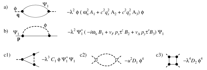
Figure 3: Diagrams entering the one-loop RG equations for cases A,B,D–F. Full lines (dashed) lines denote fermionic (bosonic) propagators, filled (open) circles represent the $\lambda_{0}$ ($u_{0}$) interaction. The constants $A_{i}$, … are obtained by evaluating the diagrams, expanding to lowest non-trivial order in the external momentum and taking the $\Lambda(d/d\Lambda)$ derivative as described in the text. a) and b) are the velocity renormalizations whereas c) contains the renormalized couplings. (Diagrams for $\Psi_{2}$ are similar.)

We demonstrate this method by calculating the linear-order fermionic self-energy $\Sigma_{\Psi_{1}}$ for the cases A,B,D–F. The diagram shown in Fig 3b evaluates to

$$\Sigma_{\Psi_{1}}({\bf q})=\lambda_{0}^{2}\int_{0}^{\infty}\!\frac{p^{2}dp}{8\pi^{3}}\int\!d\Omega_{n}K\!\!\left(\frac{p^{2}}{\Lambda^{2}}\right)K\!\!\left(\frac{(\bf{p}\!-\!\bf{q})^{2}}{\Lambda^{2}}\right)\frac{ip_{1}+s_{2}v_{F}p_{2}\tau^{z}+s_{3}v_{\Delta}p_{3}\tau^{x}}{(p_{1}^{2}+v_{F}^{2}p_{2}^{2}+v_{\Delta}^{2}p_{3}^{2})(\bf{p}-\bf{q})^{2}}\,.$$

For $\Sigma_{\Psi_{1}}$ each vertex contains the coupling matrix $M_{1}$, the signs $s_{2}$, $s_{3}=\pm 1$ are therefore given by $M_{1}\tau^{z}M_{1}=s_{2}\tau^{z}$, $M_{1}\tau^{x}M_{1}=s_{3}\tau^{x}$. Expanding the above expression to linear order in ${\bf q}$ gives:

$$\Sigma_{\Psi_{1}}(\bf{q}) = 2\lambda_{0}^{2}\int_{\mu}^{\infty}\frac{dp}{8\pi^{3}}\left[\frac{-p^{2}K(p^{2}/\Lambda^{2})K^{\prime}(p^{2}/\Lambda^{2})+\Lambda^{2}K^{2}(p^{2}/\Lambda^{2})}{p^{2}\Lambda^{2}}\right]$$ (11)

$$~{}~{}~{}~{}~{}~{}~{}~{}~{}\times\int d\Omega_{n}\frac{in_{1}^{2}q_{1}+s_{2}v_{F}n_{2}^{2}q_{2}\tau^{z}+s_{3}v_{\Delta}n_{3}^{2}q_{3}\tau^{x}}{n_{1}^{2}+v_{F}^{2}n_{2}^{2}+v_{\Delta}^{2}n_{3}^{2}}\,.$$

We have inserted a lower limit $\mu$ in the $p$ integral representing an external momentum to regularized the infrared divergence. Note that the only quantity entering the RG equations is the $\Lambda(d/d\Lambda)$ derivative of the self-energy. This removes the infrared divergence, i.e., we can take the limit $\Lambda/\mu\rightarrow\infty$ in the final expression. Writing the cut-off integral involving $K$ in general dimension $D$ we obtain

$$\Lambda\frac{d}{d\Lambda}\Sigma_{\Psi_{1}} = \frac{2\lambda_{0}^{2}K_{1}}{(2\pi)^{D}\Lambda^{4-D}}\int d\Omega_{n}\frac{in_{1}^{2}q_{1}+s_{2}v_{F}n_{2}^{2}q_{2}\tau^{z}+s_{3}v_{\Delta}n_{3}^{2}q_{3}\tau^{x}}{n_{1}^{2}+v_{F}^{2}n_{2}^{2}+v_{\Delta}^{2}n_{3}^{2}}\,,$$ (12)

$$K_{1} = \int_{0}^{\infty}dy\,y^{(D-4)/2}\left[-K(y)K^{\prime}(y)+y[K^{\prime}(y)]^{2}+yK(y)K^{\prime\prime}(y)\right]\,.$$

A simple integration by parts for $D=4$ shows that $K_{1}$ equals unity, independent of $K(y)$.

At this point it is useful to introduce dimensionless coupling constants $\lambda$ and $u$ by $\lambda_{0}=\lambda\,\Lambda^{\epsilon/2}/S_{D}^{1/2}$ and $u_{0}=u\,\Lambda^{\epsilon}/S_{D}$ with $S_{D}=\Omega_{D}/(2\pi)^{D}=2/[\Gamma(D/2)(4\pi)^{D/2}]$ and $\Omega_{D}$ being the area of a $D$-dimensional unit sphere. From Eq (12) we can easily read off the values of the $B_{i}$:

$$B_{i}=-2K_{1}\int\frac{d\Omega_{n}}{\Omega_{D}}\,\frac{s_{i}n_{i}^{2}}{n_{1}^{2}+v_{F}^{2}n_{2}^{2}+v_{\Delta}^{2}n_{3}^{2}}$$ (13)

with $s_{1}=-1$. The other diagrams in Fig 3 are evaluated similarly.

The derivation of the RG equations is straightforward and essentially identical to the momentum shell method. We construct flow equations for all velocities and couplings to one-loop order in the non-linearities $\lambda$, $u$. It is convenient to choose the time scale such that $c=1$ at each step (this introduces a non-trivial dynamical critical exponent $z$). The procedure results in the following RG equations for cases A,B,D–F:

$$\beta(v_{F}) = -v_{F}\lambda^{2}\left(B_{2}-B_{1}+\frac{\bar{A_{1}}-\bar{A_{2}}}{2}\right)\,,$$

$$\beta(v_{\Delta}) = -v_{\Delta}\lambda^{2}\left(B_{3}-B_{1}+\frac{\bar{A_{1}}-\bar{A_{2}}}{2}\right)\,,$$

$$\beta(\lambda) = -\frac{\epsilon}{2}\lambda+\lambda^{3}\left(\frac{3\bar{A_{2}}-\bar{A_{1}}}{4}+B_{1}-C_{1}\right)\,,$$

$$\beta(u) = -\epsilon u+\frac{\lambda^{2}u}{2}(\bar{A_{1}}+3\bar{A_{2}})-\frac{u^{2}}{24}D_{1}-24\lambda^{4}D_{2}$$ (14)

with the renormalization constants as defined in Fig 3 and $\bar{A_{1}}=2A_{1}$, $\bar{A_{2}}=A_{2}+A_{3}$. At a fixed point the dynamical critical exponent $z$ and the anomalous field dimensions are given by

$$z = 1+\lambda^{\ast 2}(\bar{A_{1}}-\bar{A_{2}})/2\,,$$

$$\eta_{b} = \lambda^{\ast 2}\bar{A_{2}}\,,$$

$$\eta_{f} = \lambda^{\ast 2}\left[B_{1}-(\bar{A_{1}}-\bar{A_{2}})/2\right]\,.$$ (15)

From Eq (14) we see that $\beta(v_{F})=\beta(v_{\Delta})=0$ requires $B_{2}=B_{3}$ at a non-trivial fixed point. The signs of the $B_{i}$ (13) are determined by $s_{i}$, and this preempts a fixed point for the cases D–F: the structure of $M_{1,2}$ leads to $s_{2}=-s_{3}$, so that $B_{2}$ and $B_{3}$ have always different signs.

The cases A and B have $s_{2}=s_{3}=-1$, and it is easy to show that the fixed point equations for $v_{F}$ and $v_{\Delta}$ are simultaneously satisfied only for $v_{F}^{\ast}=v_{\Delta}^{\ast}=1$. This implies that the resulting fixed point is Lorentz invariant [3]; for $D=4$ the renormalization constants are given by $\bar{A}_{1,2}=4$, $B_{i}=1/2$, $C_{1}=-1$, $D_{1}=-36$, $D_{2}=2$. The RG equations have the infrared stable fixed point [3] with $z=1$ and

$$\lambda^{\ast 2}=\frac{\epsilon}{7}\,,~{}~{}u^{\ast}=\frac{16\epsilon}{21}\,.$$ (16)

Let us briefly discuss the remaining case G. By choosing the time scale we keep the velocity $c_{1}=1$ fixed. The flow equations for $v_{F}$, $v_{\Delta}$, and $\lambda$ have the same form as above, but with $\bar{A}_{1,2}$ replaced by $A_{1,2}$, since each fermion field couples to only one species of bosons. The other RG equations read:

$$\beta(e) = e\lambda^{2}A_{2}\,,~{}~{}~{}~{}~{}~{}~{}\beta(c_{2}^{2})=c_{2}^{2}\lambda^{2}(A_{3}-A_{2})\,,$$

$$\beta(u) = -\epsilon u+\frac{\lambda^{2}u}{2}(A_{1}+3A_{2})-\frac{u^{2}+v^{2}}{24}D_{1}-24\lambda^{4}D_{2}\,,$$

$$\beta(v) = -\epsilon v+\frac{\lambda^{2}v}{2}(A_{1}+3A_{2})-\frac{uv}{24}E_{1}-\frac{v^{2}}{24}E_{2}$$ (17)

where $E_{1}$ and $E_{2}$ renormalizing $v$ arise from diagrams similar to Fig 3c2. Analysis of these equations shows that $\beta(v_{F})=\beta(v_{\Delta})=\beta(c_{2}^{2})=0$ is only fulfilled for $c_{2}=1$ and $v_{F}=v_{\Delta}$. Furthermore we must have $e=0$ at a fixed point, stability requires $A_{2}>0$. Explicit evaluation in $D=4$ shows that the zeros of $\beta(v_{F})$ have $A_{2}<0$ which proves the non-existence of a fixed point for case G.

We summarize this subsection by restating the main conclusions. Among the ${\bf Q}=0$ order parameters considered here, only cases A and B possess stable RG fixed points which can describe a second-order quantum phase transition to the state $X$, and with strong damping of quasiparticle spectral functions. The fixed points for both cases are Lorentz invariant, and for future convenience, we display this explicitly. We perform the unitary transformation

$$\Psi_{2a}=\frac{(\tau^{x}+\tau^{z})}{\sqrt{2}}\Psi_{\dot{2}a}$$ (18)

(this ensures that the structure of the $\tau$ matrices in (3) is the same for $\Psi_{1}$ and $\Psi_{\dot{2}}$), define $\overline{\Psi}_{1,\dot{2}a}=-i\tau^{y}\Psi_{1,\dot{2}a}^{\dagger}$, and introduce the Lorentz index $\mu=\tau,x,y$. Then $S_{\Psi}+S_{\phi}+S_{\Psi\phi}$ can be written as

$$S_{1} = \int d^{3}x\Big{(}i\overline{\Psi}_{1a}\partial_{\mu}\gamma^{\mu}\Psi_{1a}+i\overline{\Psi}_{\dot{2}a}\partial_{\mu}\gamma^{\mu}\Psi_{\dot{2}a}+\frac{1}{2}(\partial_{\mu}\phi)^{2}+\frac{r}{2}\phi^{2}+\frac{u_{0}}{24}\phi^{4}$$ (19)

$$~{}~{}~{}~{}~{}~{}~{}~{}~{}~{}~{}~{}~{}~{}~{}~{}~{}~{}~{}~{}~{}~{}~{}~{}~{}~{}~{}~{}~{}~{}~{}~{}~{}~{}-i\lambda_{0}\phi(\overline{\Psi}_{1a}\Psi_{1a}\mp\overline{\Psi}_{\dot{2}a}\Psi_{\dot{2}a})\Big{)},$$

where $\gamma^{\mu}=(-\tau^{y},\tau^{x},\tau^{z})$, we have set $v_{F}=v_{\Delta}=c=1$ and the $-$ ($+$) sign in the last term is for case A (B).

2.2 Order parameters with ${\bf Q}=(2K,2K)$

One plausible candidate for ordering at such a wavevector is antiferromagnetic order at ${\bf Q}=(\pi,\pi)$, $K=\pi/2$; this case was discussed in Section 1, and has been analyzed by Balents et al. [14] (The generalization to magnetic order at incommensurate wavevectors is not difficult, but we will not consider it because incommensuration along the diagonal direction in the Brillouin zone has not been observed in the superconducting cuprates.) We represent the strength of the antiferromagnetic order by a real, three-component field $N_{\alpha}$ ($\alpha=x,y,z$; for the incommensurate case $N_{\alpha}$ is complex). The transition from a $d$-wave superconductor with $\langle N_{\alpha}\rangle=0$ to a state $X$ which is a $d$-wave superconductor with $\langle N_{\alpha}\rangle\neq 0$ is described by the following continuum action near the critical point [14]

$$S_{2} = \int d^{3}x\Big{(}i\overline{\Psi}_{1a}\partial_{\mu}\gamma^{\mu}\Psi_{1a}+i\overline{\Psi}_{\dot{2}a}\partial_{\mu}\gamma^{\mu}\Psi_{\dot{2}a}+\frac{1}{2}(\partial_{\mu}N_{\alpha})^{2}+\frac{r}{2}N_{\alpha}^{2}+\frac{u_{0}}{24}(N_{\alpha}^{2})^{2}$$ (20)

$$~{}~{}~{}~{}~{}~{}~{}~{}~{}+i\lambda_{0}N_{\alpha}\varepsilon_{ac}\sigma^{\alpha}_{cb}\left[\Psi_{1a}{\cal C}\Psi_{1b}-\Psi_{\dot{2}a}{\cal C}\Psi_{\dot{2}b}+\mbox{H.c.}\right]\Big{)},$$

where $\sigma^{\alpha}$ are Pauli matrices in spin space, and ${\cal C}=i\tau^{y}$ is a matrix in Nambu space. Like $S_{1}$, $S_{2}$ has the property of Lorentz invariance ($\Psi{\cal C}\Psi$ and $\overline{\Psi}\Psi$ are Lorentz scalars). Also like $S_{1}$, the couplings $\lambda$ and $u$ approach [14] fixed point values under the RG, and so the fermion spectral function in the quantum-critical region will have an energy width of order $k_{B}T$.

For completeness, we mention another order parameter at ${\bf Q}=(\pi,\pi)$ which has been the focus of some recent discussion: the staggered flux order [17]. The coupling of this order to the nodal fermions involves a spatial derivative, and can be shown to be irrelevant: [3] so the fermionic quasiparticles are merely spectators at a transition involving the onset of staggered flux order and such a theory is not of interest here.

2.3 Order parameter with ${\bf Q}=(2K,0),(0,2K)$

An attractive possibility of an order parameter with such a ${\bf Q}$ is the charge density itself (or ‘charge stripe’ order). We consider the incommensurate case, in which the charge density has the modulation

$$\delta\rho=\mbox{Re}\left[\Phi_{x}e^{i2Kx}+\Phi_{y}e^{i2Ky}\right]$$ (21)

where $\Phi_{x,y}$ are complex fields which constitute the charge-stripe order parameter. Related order parameters have been considered earlier by Castellani et al [18], but they discussed the onset of charge density wave order in a Fermi liquid (for this case $K$ has no meaning, and one considers instead charge density wave order at a generic ${\bf Q}$ which can connect two points on the Fermi surface), whereas we will consider the onset in a $d$-wave superconductor. The theories for the two cases are very different: the former has an overdamped spectrum for the order parameter fluctuations [19] and (because the theory is not below its upper-critical dimension) does not satisfy the strong scaling properties assumed for the fermion spectral functions to be discussed in Section 3, which do apply to the latter. We believe it is important to discuss the onset of charge order in the true ground state of the doped antiferromagnet, the $d$-wave superconductor, and hence our focus on this case.

The field theory for a transition from a $d$-wave superconductor to a state $X$ which is a $d$-wave superconductor co-existing with the modulation (21) can be deduced [13, 3] as in the cases above, and near the critical fixed point it takes the form

$$S_{3} = \int d^{3}x\Big{(}i\overline{\Psi}_{1a}\partial_{\mu}\gamma^{\mu}\Psi_{1a}+i\overline{\Psi}_{\dot{2}a}\partial_{\mu}\gamma^{\mu}\Psi_{\dot{2}a}+|\partial_{\mu}\Phi_{x}|^{2}+|\partial_{\mu}\Phi_{y}|^{2}+r\left(|\Phi_{x}|^{2}+|\Phi_{y}|^{2}\right)$$ (22)

$$\!\!\!\!\!\!\!\!\!\!\!+\frac{u_{0}}{2}\left(|\Phi_{x}|^{4}\!+\!|\Phi_{y}|^{4}\right)+v_{0}|\Phi_{x}|^{2}|\Phi_{y}|^{2}+\lambda_{0}\!\left[\Phi_{x}\overline{\Psi}_{\dot{2}a}\Psi_{1a}\!-\!\Phi_{y}\varepsilon_{ab}\Psi_{\dot{2}a}{\cal C}\Psi_{1b}\!+\!\mbox{H.c.}\right]\Big{)}.$$

The RG properties [3] of $S_{3}$ are very similar to the cases $S_{1,2}$ considered previously: $u$, $v$, and $\lambda$ approach fixed point values, and there is a universal coupling between fermionic and bosonic fluctuations in the critical region.

3 Fermion spectral functions

The remainder of this paper will highlight some important observable properties of the field theories $S_{1,2,3}$ in (19,20,22). We will restrict ourselves to the scaling limit, both at $T=0$ and $T>0$; for some quantities we will see that it is necessary to consider corrections to scaling to obtain a complete picture—we will not enter into such issues here and leave them for future work.

In this section we consider single fermion Green’s functions which can be measured in photoemission experiments. In the quantum-critical region (Fig  1) of $S_{1,2,3}$ these will obey

$$G_{f}(k,\omega)=\frac{{\cal A}_{f}}{T^{(1-\eta_{f})}}\,\Phi_{f}\!\left(\frac{\omega}{T},\frac{k}{T}\right),$$ (23)

where we have set $\hbar$, $k_{B}$ and all velocities to unity. The scale factor ${\cal A}_{f}$ is non-universal, while the exponent $\eta_{f}$ and the complex-valued function $\Phi_{f}$ are universal and depend only upon whether the relevant theory is $S_{1}$, $S_{2}$ or $S_{3}$. Scaling functions like $\Phi_{f}$ have been studied by a variety of approximate methods [20], and we will quote some useful limiting forms here (in contrast, in 1+1 dimensions exact results for analogous scaling functions are known [20, 21] for all values of their arguments).

For $\omega,k\gg T$, (23) reduces to [14, 3]

$$G_{f}(k,\omega)={\cal A}C_{f}\frac{\omega+k_{x}\tau^{z}+k_{y}\tau^{x}}{\left[k^{2}-(\omega+i0)^{2}\right]^{1-\eta_{f}/2}},$$ (24)

where $C_{f}$ is a universal number. Note that the imaginary part of this is non-zero only for $\omega>k$, and it decays as $\omega^{-1+\eta_{f}}$ for large $\omega$; a similar kinematic constraint and large $\omega$ tail was noted recently in one-dimensional stripe models for fermion spectral functions [21]. The expression (24) has a singularity precisely at $\omega=k$: this singularity is rounded at any non-zero $T>0$ and so (24) is not an accurate representation of (23) right at the threshold. Unfortunately, the nature of this rounding is not easy to compute in general; it can be computed in an expansion in $\eta_{f}$, and these results are in Appendix A of our recent work [3].

In the opposite limit, $\omega,k\ll T$, (23) has a very different form. Now the $k$ and $\omega$ dependencies are smooth, and all anomalous powers involve only factors of $T$. The following approximate form was suggested [3] in this limit

$$G_{f}(k,\omega)={\cal A}T^{\eta_{f}}\frac{\omega+i\Gamma_{f}+k_{x}\tau^{z}+k_{y}\tau^{x}}{k^{2}-(\omega+i\Gamma_{f})^{2}},$$ (25)

where the overall scale of the right hand side defines the value of ${\cal A}$, and $\Gamma_{f}/T$ is a universal number. Estimates of this universal number have been given for $S_{1,3}$. Note that along the diagonal direction in the Brillouin zone ($k_{x}=0$), the result (25) predicts a simple Lorentzian for the spectral function with an energy width of order $\Gamma_{f}$. Of course, the Lorentzian form breaks down for large $\omega$, when the spectral function crosses over to the slowly decaying tail predicted by (24).

4 Transport properties

Unlike the single-particle properties of Section 3, transport properties can require determination of composite correlators of both the fermionic and bosonic degrees of freedom. In particular, we can have processes in which there is rapid scattering between fermions and bosons, and thus a broad fermion spectral function, but essentially no degradation of the transport current. In such cases, it is clearly not appropriate to interpret transport properties in terms of a single fermionic quasiparticle lifetime, and attempts to do so will suggest very long quasiparticle lifetimes very different from those observed in photoemission experiments.

We describe spin, thermal, and charge transport in the following subsections:

4.1 Spin transport

The global $SU(2)$ spin-rotation symmetry of $S_{1,2,3}$ implies that total spin is conserved. Consequently, there is an associated Lorentz 3-current, $J^{s\alpha}_{\mu}$ obeying $\partial_{\mu}J^{s\alpha}_{\mu}=0$. For $S_{1,3}$ this 3-current has only a fermionic contribution

$$J^{s\alpha}_{\mu}=\frac{1}{2}\left[\overline{\Psi}_{1a}\sigma^{\alpha}_{ab}\gamma_{\mu}\Psi_{1b}+\overline{\Psi}_{\dot{2}a}\sigma^{\alpha}_{ab}\gamma_{\mu}\Psi_{\dot{2}b}\right]$$ (26)

(this expression agrees with earlier work [22]), while for $S_{2}$ there is also bosonic contribution [20]

$$J^{s\alpha}_{\mu}=\frac{1}{2}\left[\overline{\Psi}_{1a}\sigma^{\alpha}_{ab}\gamma_{\mu}\Psi_{1b}+\overline{\Psi}_{\dot{2}a}\sigma^{\alpha}_{ab}\gamma_{\mu}\Psi_{\dot{2}b}\right]+i\epsilon_{\alpha\beta\gamma}N_{\beta}\partial_{\mu}N_{\gamma}.$$ (27)

The conservation of $J^{s\alpha}_{\mu}$ implies that the total spin is a constant of motion

$$\frac{d}{d\tau}\int d^{2}xJ^{s\alpha}_{\tau}=0;$$ (28)

however, the physical spin current is not conserved:

$$\frac{d}{d\tau}\int d^{2}xJ^{s\alpha}_{x,y}\neq 0.$$ (29)

The spin conductivity, $\sigma_{s}$, is expressed by a Kubo formula involving $J^{s\alpha}_{x,y}$ (along with a ‘diamagnetic’ contact term for the bosonic fields in $S_{2}$) and (29) implies that a ballistic contribution to $\sigma_{s}$ is not expected. The scaling properties of $\sigma_{s}$ can be deduced along the lines discussed [20] for a purely bosonic theory: the conservation of the 3-current implies that the scaling dimension of $\sigma_{s}$ is protected to take the value $d-2=0$, and so in the quantum critical region we have [20, 8]

$$\sigma_{s}=\Phi_{s}\left(\frac{\omega}{T}\right),$$ (30)

where $\Phi_{s}$ is a universal function of order unity (we have absorbed factors of $g\mu_{B}$ in the definition of $\sigma_{s}$). In principle, it should not be difficult to extend earlier results [20] for purely bosonic theories to determine the collisionless ($\omega\gg T$) and collision-dominated ($\omega\ll T$) regimes of $\sigma_{s}$.

4.2 Thermal transport

This section is based on ideas of T. Senthil (unpublished) in a different context.

The Lorentz invariance of $S_{1,2,3}$ implies the existence of a energy-momentum 3-tensor $\Theta_{\mu\nu}$ which is conserved, $\partial_{\mu}\Theta_{\mu\nu}=0$, and which can be chosen to symmetric in the $\mu,\nu$ indices [23]. The energy density is $\Theta_{\tau\tau}$, while the energy current is $J^{e}_{i}=\Theta_{i\tau}$, where $i=x,y$. The conservation of the 3-tensor $\Theta_{\mu\nu}$ implies three constants of motion, the total energy and the total momentum:

$$\frac{d}{d\tau}\int d^{2}x\Theta_{\tau\nu}=0.$$ (31)

Now using the symmetry of $\Theta_{\mu\nu}$, and in particular $\Theta_{i\tau}=\Theta_{\tau i}$, we conclude that the spatial integral of the energy current $J^{e}_{i}$ is also conserved [contrast this with (29), in which the spatial integral over the spin current was not conserved]. As the thermal conductivity is given by a Kubo formula involving the energy current, we conclude that heat transport is ballistic and the thermal conductivity is infinite in the scaling limits defined by $S_{1,2,3}$.

4.3 Charge transport

The above theories describe excitations in superconductors, and a complete description of charge transport, and an accounting of the conservation of total charge, requires inclusion of the Cooper pairs [alternatively stated, we have to include the fluctuations of $\varphi$ in (1)]. However, in a frequency regime where the response is dominated by quasiparticle excitations, we can consider the predictions of $S_{1,2,3}$ alone. The quasiparticle contribution to the electrical current is [22] the 2-vector $J^{c}_{i}=(\Psi_{1a}^{\dagger}\Psi_{1a},\Psi_{2a}^{\dagger}\Psi_{2a})=i(\overline{\Psi}_{1}\gamma_{\tau}\Psi_{1},-\overline{\Psi}_{\dot{2}a}\gamma_{\tau}\Psi_{\dot{2}a})$. In general there is nothing special about this operator: it will acquire anomalous dimensions at the critical point, and this will lead to a contribution to the charge conductivity which has prefactors of a non-universal constant and an anomalous power of $T$. However, for the case of $S_{1}$ only, an exceptional circumstance occurs: the action has $U(1)$ symmetries corresponding to global changes in the phases of $\Psi_{1,\dot{2}}$, and corresponding conserved 3-currents $\partial_{\mu}\overline{\Psi}_{1a}\gamma_{\mu}\Psi_{1a}=\partial_{\mu}\overline{\Psi}_{\dot{2}a}\gamma_{\mu}\Psi_{\dot{2}a}=0$. Note that these 3-currents do not correspond to the conservation of physical electrical charge: rather, the $\tau$ component of these 3-currents happen to be equal to the $x,y$ components of the electrical current $J^{c}_{i}$. The conservations of these currents implies that the spatial integral of $J^{c}_{i}$ is a constant of motion, and hence the quasiparticle contribution to the charge conductivity is a zero-frequency delta function for $S_{1}$.

5 Conclusion

This paper has identified quantum field theories at which the nodal quasiparticles of a $d$-wave superconductor undergo strong inelastic scattering. All these theories are associated with a quantum critical point between a $d$-wave superconductor and some other superconducting state $X$ (Fig 1). We performed an exhaustive search among states $X$ associated with a spin-singlet, zero momentum, fermion bilinear order parameter, and found that only two candidates possessed a non-trivial quantum critical point: $X$ a $d_{x^{2}-y^{2}}+is$ or a $d_{x^{2}-y^{2}}+id_{xy}$ superconductor. The quantum field theory for these cases is $S_{1}$ in (19). Among order parameters with a non-zero momentum, we had to permit a fine-tuning condition that the ordering momentum was equal to the spacing between two Fermi points of the $d$-wave superconductor. Two plausible cases of this kind had $X$ possessing co-existing spin-density wave order and $d$-wave superonductivity [described by $S_{2}$ in (20)] or co-existing charge-density wave order and $d$-wave superconductivity [described by $S_{3}$ in (22)].

We reviewed the single particle (Section 3) and transport (Section 4) properties of $S_{1,2,3}$. An important observation was that there is no simple relationship between the relaxation times associated with these observables. In particular, strong scattering between the fermionic and bosonic modes can lead to very short single particle lifetimes and broad spectral functions (Section 3). At the same time, these scattering processes can do little to degrade the transport current: the thermal conductivity of $S_{1,2,3}$ was found to be infinite in the continuum scaling limit.

Comparison of the above results with experiments requires some understanding of the effects of corrections to scaling, and of impurity scattering. Initial steps in this direction have been taken [3], and studies for transport properties are in progress.

Keeping the above cautions in mind, we offer a possible interpretation of recent thermal conductivity measurements [2]. A strong enhancement of the thermal Hall conductivity, $\kappa_{xy}$, is observed as $T$ is lowered, but $\kappa_{xy}$ saturates and decreases below $T=28$ K. The enhancement suggests large fluctuations of chiral order[24], as is the case when $X$ is a $d_{x^{2}-y^{2}}+id_{xy}$ superconductor (for $T<T_{X}$ this state has a non-zero $\kappa_{xy}$ even in zero field [25]). So we suggest that the experimental system is in the vicinity of such a state $X$ but has $r>r_{c}$, and the crossover at the dashed line in Fig 1 occurs at $T\approx 28$ K. A testable implication is that the photoemission linewidths of the nodal fermions should be $\sim k_{B}T$ down to 28 K, and then cross over to behavior expected in an ordinary BCS $d_{x^{2}-y^{2}}$ superconductor at lower $T$.

References

In the discussion of case G in our paper[1], above Eq. (4), the single sentence “The state $X$ retains $\mathcal{T}$ and the gapless nodal points, but has $C_{4v}$ broken to $Z_{2}$” is incorrect. The state $X={\rm G}$ breaks $\mathcal{T}$ (time-reversal), and has spontaneous electrical currents. For $\phi_{x}\neq 0$ and $\phi_{y}=0$ (or vice versa) the currents have the same symmetry as those in the state $\Theta_{\rm II}$ discussed by Simon and Varma [2]. Also, as pointed out by Berg et al. [3], the nodal quasiparticles do not survive in the superconducting state G, but turn into Fermi pockets. The latter conclusion can be verified from the fermion spectrum obtained by diagonalizing Eqs. (1)+(5) for constant $\phi_{x,y}$.

All other sentences and the conclusions in the paper [1] remain unchanged.

Also, in the companion paper[4], the only error is in the sketch of the fermion excitations in Fig. 2 for case G.

We thank Erez Berg and Cenke Xu for helpful discussions. This research was supported by NSF grant DMR-0537077 and DFG SFB 608.

References

- [*] New permanent address: Theoretische Physik III, Elektronische Korrelationen und Magnetismus, Universität Augsburg, D-86135 Augsburg, Germany.
- [1] T. Valla, A. V. Fedorov, P. D. Johnson, B. O. Wells, S. L. Hulbert, Q. Li, G. D. Gu, and N. Koshizuka, Science 285, 2110 (1999).
- [2] Y. Zhang, N. P. Ong, P. W. Anderson, D. A. Bonn, R. Liang, and W. N. Hardy, preprint; K. Krishana, J. M. Harris, and N. P. Ong, Phys. Rev. Lett. 75, 3529 (1995).
- [3] M. Vojta, Y. Zhang, and S. Sachdev, Phys. Rev. B Sep 1 (2000), cond-mat/0003163.
- [4] M. Vojta, Y. Zhang, and S. Sachdev, cond-mat/0007170.
- [5] S. Chakravarty, B. I. Halperin, and D. R. Nelson, Phys. Rev. Lett. 60, 1057 (1988); Phys. Rev. B 39, 2344 (1989).
- [6] N. Read and S. Sachdev, Phys. Rev. Lett. 62, 1694 (1989); 66, 1773 (1991); G. Murthy and S. Sachdev, Nucl. Phys. B 344, 557 (1990).
- [7] S. Sachdev and J. Ye, Phys. Rev. Lett. 69, 2411 (1992); A. V. Chubukov and S. Sachdev, ibid. 71, 169 (1993); A. V. Chubukov, S. Sachdev, and J. Ye, Phys. Rev. B 49, 11919 (1994).
- [8] S. Sachdev, Science 288, 475 (2000).
- [9] H. Alloul, P. Mendels, G. Collin, and P. Monod, Phys. Rev. Lett. 61, 746 (1988); M. Takigawa, P. C. Hammel, R. H. Heffner, Z. Fisk, J. L. Smith, and R. B. Schwarz, Phys. Rev. B 39, 300 (1989); T. Imai, C. P. Slichter, K Yoshimura, and K. Kosuge, Phys. Rev. Lett. 70, 1002 (1993); T. Imai, C. P. Slichter, K. Yoshimura, M. Katoh, K. Kosuge, ibid. 71, 1254 (1993); A. Sokol and D. Pines, ibid. 71, 2813 (1993); Y. Zha, V. Barzykin, and D. Pines Phys. Rev. B 54, 7561 (1996); A. W. Hunt, P. M. Singer, K. R. Thurber, T. Imai, ibid. 82, 4300 (1999); S. Fujiyama, M. Takigawa, Y. Ueda, T. Suzuki, N. Yamada, Phys. Rev. B 60, 9801 (1999).
- [10] G. Aeppli, T. E. Mason, S. M. Hayden, H. A. Mook, and J. Kulda, Science 278, 1432 (1997); S. M. Hayden, G. Aeppli, H. A. Mook, D. Rytz, M. F. Hundley, and Z. Fisk, Phys. Rev. Lett. 66, 821 (1991); B. Keimer, N. Belk, R. J. Birgeneau, A. Cassanho, C. Y. Chen, M. Greven, M. A. Kastner, A. Aharony, Y. Endoh, R. W. Erwin, and G. Shirane, Phys. Rev. B 46, 14034 (1992).
- [11] P. W. Anderson, cond-mat/0007185.
- [12] J. Rossat-Mignod, L. P. Regnault, C. Vettier, P. Bourges, P. Burlet, J. Bossy, J. Y. Henry, and G. Lapertot, Physica C 185-189, 86 (1991); H. A. Mook, M. Yehiraj, G. Aeppli, T. E. Mason, and T. Armstrong, Phys. Rev. Lett. 70, 3490 (1993); H. F. Fong, B. Keimer, F. Dogan, and I. A. Aksay, ibid. 78, 713 (1997); P. Bourges in The Gap Symmetry and Fluctuations in High Temperature Superconductors ed. J. Bok, G. Deutscher, D. Pavuna, and S. A. Wolf, Plenum, New York (1998) pp. 349-371, cond-mat/9901333; P. Dai, H. A. Mook, S. M. Hayden, G. Aeppli, T. G. Perring, R. D. Hunt, and F. Dogan Science 284, 1344 (1999); H. F. Fong, P. Bourges, Y. Sidis, L. P. Regnault, J. Bossy, A. Ivanov, D. L. Milius, I. A. Aksay, and B. Keimer, Phys. Rev. Lett. 82, 1939 (1999); P. Bourges, Y. Sidis, H. F. Fong, L. P. Regnault, J. Bossy, A. Ivanov, and B. Keimer, Science 288, 1234 (2000); Y. Sidis, P. Bourges, H. F. Fong, B. Keimer, L. P. Regnault, J. Bossy, A. Ivanov, B. Hennion, P. Gautier-Picard, G. Collin, D. L. Millius, and I. A. Aksay, Phys. Rev. Lett. 84, 5900 (2000).
- [13] M. Vojta and S. Sachdev, Phys. Rev. Lett. 83, 3916 (1999).
- [14] L. Balents, M. P. A. Fisher, and C. Nayak, Int. J. Mod. Phys. B 12, 1033 (1998).
- [15] We will not consider the cases where the separation between nodal points is an integer multiple of , because the order-parameter/fermion coupling is then found to be irrelevant by power-counting [3].
- [16] E. Brézin, J. C. Le Guillou, J. Zinn-Justin in Phase Transitions and Critical Phenomena, vol 6, C. Domb and M. S. Green eds, Academic Press, London (1976); the method used by us is discussed in Section 5.
- [17] D. A. Ivanov, P. A. Lee, and X.-G. Wen, Phys. Rev. Lett. 84, 3958 (2000); S. Chakravarty, R. B. Laughlin, D. K. Morr, and C. Nayak, cond-mat/0005443.
- [18] C. Castellani, C. DiCastro, and M. Grilli, Phys. Rev. Lett. 75, 4650 (1995); S. Caprara, M. Sulpizi, A. Bianconi, C. Di Castro, and M. Grilli, Phys. Rev. B 59, 14980 (1999).
- [19] J. A. Hertz, Phys. Rev. B 14, 1165 (1976).
- [20] S. Sachdev, Quantum Phase Transitions, Cambridge University Press, Cambridge (1999).
- [21] D. Orgad, S. A. Kivelson, E. W. Carlson, V. J. Emery, X. J. Zhou, and Z. X. Shen, cond-mat/0005457.
- [22] A. C. Durst and P. A. Lee, Phys. Rev. B 62, 1270 (2000).
- [23] S. Weinberg, The Quantum Theory of Fields, vol 1, Cambridge University Press, Cambridge (1995), Section 7.4.
- [24] G. Kotliar, A. M. Sengupta, and C. M. Varma Phys. Rev. B 53, 3573 (1996).
- [25] T. Senthil, J. B. Marston, and M. P. A. Fisher, Phys. Rev. B 60, 4245 (1999).

References

- [1] M. Vojta, Y. Zhang, and S. Sachdev, Phys. Rev. Lett. 85, 4940 (2000).
- [2] M. E. Simon and C. M. Varma, Phys. Rev. Lett. 89, 247003 (2002), see Fig 1b.
- [3] E. Berg, C.-C. Chen, and S. A. Kivelson, Phys. Rev. Lett. 100, 027003 (2008).
- [4] M. Vojta, Y. Zhang, and S. Sachdev, Int. J. Mod. Phys. B 14, 3719 (2000) [arXiv:cond-mat/0008048].