Signatures of Spin and Charge Energy Scales
in the Local Moment and Specific Heat
of the Two–Dimensional Hubbard Model

Abstract

Local moment formation driven by the on–site repulsion $U$ is one of the most fundamental features in the Hubbard model. At the simplest level, the temperature dependence of the local moment is expected to have a single structure at $T\sim U$, reflecting the suppression of the double occupancy. In this paper we show new low temperature Quantum Monte Carlo data which emphasize that the local moment also has a signature at a lower energy scale which previously had been thought to characterize only the temperatures below which moments on different sites begin to correlate locally. We discuss implications of these results for the structure of the specific heat, and connections to quasiparticle resonance and pseudogap formation in the density of states.

]

I Introduction

The finite temperature properties of the two dimensional Hubbard model have been extensively studied both analytically and numerically.[1] Quantum Monte Carlo (QMC) is especially effective at half-filling, where there is no sign problem. From calculations of the magnetic structure factor, susceptibility, compressibility, density of states, and the electron self–energy, a clear picture has emerged concerning the nature of the short and long range magnetic order, the Mott gap, and the quasiparticle dispersion.

While the specific heat $C(T)$ has been computed by a number of groups in one-dimension, principally by Bethe Ansatz techniques[2], there have been few QMC studies of $C(T)$ for the two and three dimensional Hubbard models.[3, 4, 5] The behavior for large $U$ is well understood and one expects, as in the one dimensional case, a two peak structure in $C(T)$, with a broad high temperature peak at $T\sim U$ associated with “charge fluctuations”, and a narrower peak at lower temperatures associated with “spin fluctuations”.

This two peak structure of the Hubbard model can be understood from a strong coupling viewpoint as follows: At temperatures which exceed the on–site repulsion, $T>U$, the up and down electrons are decoupled, $\langle n_{\uparrow}n_{\downarrow}\rangle=\langle n_{\uparrow}\rangle\langle n_{\downarrow}\rangle=\frac{1}{4}$, at half–filling, and the local moment $\langle m_{z}^{2}\rangle=\langle(n_{\uparrow}-n_{\downarrow})^{2}\rangle=\langle n_{\uparrow}+n_{\downarrow}-2n_{\uparrow}n_{\downarrow}\rangle=1-\langle n_{\uparrow}n_{\downarrow}\rangle=0.5$, its uncorrelated value. At the temperature scale $T\sim U$, double occupancy begins to be suppressed, $\langle n_{\uparrow}n_{\downarrow}\rangle\rightarrow 0$, and $m_{z}^{2}\rightarrow 1$. Since the potential energy in the Hubbard model is just $P=Un_{\uparrow}n_{\downarrow}={U\over 2}(1-m_{z}^{2})$, this growth in the local moment is synonymous with a decrease in the potential energy as $T$ decreases, and hence a peak in $C(T)$ at $T\sim U$. Once moments are formed, the half–filled Hubbard model maps onto the spin–1/2 antiferromagnetic Heisenberg model, with exchange constant $J=4t^{2}/U$, whose specific heat has a peak at $T\sim J$ associated with magnetic ordering. In sum, one expects $C(T)$ for the strong coupling Hubbard model at half–filling to have a “charge peak” at $T\sim U$ and a “spin peak” at $T\sim J$. This strong coupling argument further suggests that the temperature derivatives of the potential and kinetic energies are associated with the high and low temperature specific heat peaks respectively.

On the other hand, the behavior of the specific heat for small $U$ in the two dimensional Hubbard model is still unclear. In particular, it is not known whether a two peak structure is present for all values of the interaction or if these coalesce into a single peak at small $U$. That the two peaks might merge is suggested by the fact that the charge and spin energy scales, $U$ and $t^{2}/U$, approach each other as $U$ is decreased. However, the situation is not so straightforward, because the strong coupling form for the energy scale for spin ordering crosses over to a weak coupling expression[6, 7] $t\,{\rm exp}(-2\pi\sqrt{t/U})$, which at small $U$ is still well-separated from the energy scales $t$ and $U$.

The QMC results reported in this work are consistent with such weak coupling behavior at small $U$. That is, one of our key findings is that $C(T)$ shows two distinct peaks which persist to couplings an order of magnitude less than the noninteracting bandwidth. It may be that the half-filled two-dimensional Hubbard model is unique in this respect, since, as we review below, studies in one dimension and within DMFT show a merging of the peaks at values of $U$ roughly equal to the bandwidth. Indeed, the two–dimensional half–filled Hubbard model on a square lattice has unusual nesting features in its noninteracting band structure, as well as a logarithmic divergence of its density of states at the Fermi level which have previously been noted to enhance antiferromagnetism anomalously.[6]

Whether this is the case or not, there is as yet no compelling evidence of the appearence of a weak coupling energy scale $t\,{\rm exp}(-2\pi t/U)$ in the specific heat in other dimensions. In one dimension, exact diagonalization in small chains[8] and QMC calculations[9] suggest the two peaks merge, but disagree with respect to the interaction strength at which this occurs. Exact diagonalization is limited to chains of very modest extent, and finite size effects tend to be large for small U. Meanwhile, QMC work did not reach low enough temperatures to resolve the two peaks even for large values of $U$ where they almost certainly both exist. Bethe–Ansatz calculations help clarify this issue, but focus on the large $U$ limit[10, 11, 12]. Despite these various caveats, the consensus of these approaches is that the spin and charge peaks merge at $U/t\approx 4$, the one–dimensional bandwidth. Quantum transfer matrix calculations [13] also show the merging of the two peaks at $U/t\approx 4$.

Coalescence of the specific heat peaks has also been seen in “Dynamical Mean Field Theory” (DMFT) which studies the system in the limit of high dimension.[14, 15, 16] There, the Hubbard model is studied with a Gaussian density of states of unit variance, and the spin and charge peaks are found to merge at $U\approx 1.5$. The fact that the band–width is undefined complicates comparisons with results in finite dimension, but one can still examine the ratio of $U$ to the kinetic energy per particle, which is finite for a Gaussian density of states. The value $U/t\approx 4$ in two dimensions has the same ratio of $U$ to kinetic energy as the interaction strength at which the two peak structure is lost in DMFT. However, an additional difficulty in the interpretation of the DMFT results, besides the use of a Gaussian density of states, is the restriction of the calculations to the paramagnetic phase, and therefore the neglect of antiferromagnetic fluctuations.

It is the purpose of this paper to present a detailed study of the temperature dependence of the local moment and the associated features in the specific heat for the half–filled two–dimensional Hubbard Hamiltonian. A focus of our work will be on extending the strong coupling picture of the two peak structure of $C(T)$ to intermediate and weak coupling. As we shall show, the connection of moment formation and moment ordering with the high and low temperature peaks (respectively) in the specific heat is modified. At the same time, we will describe two recently developed techniques for computing the specific heat which hold certain advantages over approaches previously used. These new techniques also allow us to compute the entropy and free energy, quantities typically not so easy to obtain with Monte Carlo. A fascinating conclusion of the DMFT studies[14, 15, 16] concerned the existence of a universal crossing point of the specific heat curves for different $U$. We shall show such a crossing occurs also in two dimensions. Finally, we will discuss results for dynamical quantities like the density of states and optical conductivity and comment on their consistency with the local moment and specific heat.

II Model and Methods

A The Hubbard Hamiltonian

The two dimensional Hubbard Hamiltonian is,

$$H = -t\sum_{\langle{\bf i},{\bf j}\rangle\sigma}(c_{{\bf i}\sigma}^{\dagger}c_{{\bf j}\sigma}^{\phantom{\dagger}}+c_{{\bf j}\sigma}^{\dagger}c_{{\bf i}\sigma}^{\phantom{\dagger}})$$ (1)

$$+ U\sum_{{\bf i}}(n_{{\bf i}\uparrow}-\frac{1}{2})(n_{{\bf i}\downarrow}-\frac{1}{2})-\mu\sum_{{\bf i}}(n_{{\bf i}\uparrow}+n_{{\bf i}\downarrow}).$$ (2)

Here $c_{{\bf i}\sigma}^{\dagger}(c_{{\bf j}\sigma}^{\phantom{\dagger}})$ are creation(destruction) operators for a fermion of spin $\sigma$ on lattice site ${\bf i}$. The kinetic energy term includes a sum over near neighbors $\langle{\bf i},{\bf j}\rangle$ on a two–dimensional square lattice, and the interaction term is written in particle–hole symmetric form so that $\mu=0$ corresponds to half–filling $\langle n_{{\bf i}\uparrow}+n_{{\bf i}\downarrow}\rangle=1$ for all Hamiltonian parameters $t,U$ and temperatures $T$. We will henceforth set the hopping parameter $t=1$.

Equal time quantities of interest in this paper include the energy, $E=\langle H\rangle$, the specific heat $C=dE/dT$, the local moment $\langle m_{z}^{2}\rangle=\langle(n_{{\bf i}\uparrow}-n_{{\bf i}\downarrow})^{2}\rangle$,[17] and the near neighbor spin–spin correlation function $\langle S_{{\bf i}}S_{{\bf i}+\hat{x}}\rangle$. To probe longer range magnetic order, we evaluate the structure factor,

$$S({\bf Q})={1\over L^{2}}\sum_{{\bf i},{\bf j}}e^{i{\bf Q}\cdot({\bf i}-{\bf j})}\langle(n_{{\bf i}\uparrow}-n_{{\bf i}\downarrow})(n_{{\bf j}\uparrow}-n_{{\bf j}\downarrow})\rangle,$$ (3)

where ${\bf Q}=(\pi,\pi)$ is the antiferromagnetic wave vector.

We also evaluate two dynamic quantities. The density of states $N(\omega)$ is given implicitly from QMC data for the imaginary time Green’s function,

$$G(\tau)={1\over N}\sum_{{\bf p}}\langle c({\bf p},\tau)c^{\dagger}({\bf p},0)\rangle=\int_{-\infty}^{+\infty}d\omega{e^{-\omega\tau}N(\omega)\over e^{-\beta\omega}+1}\,.$$ (4)

Likewise, the optical conductivity, $\sigma_{xx}(\omega)$, is related to QMC data for the imaginary time current–current correlation function,

$$\sigma_{xx}(\tau) =\langle j_{x}(\tau)j_{x}(0)\rangle=\int_{-\infty}^{+\infty}d\omega{e^{-\omega\tau}\sigma_{xx}(\omega)\over e^{-\beta\omega}-1}\,,$$ (5)

$$j_{x}(\tau) =-it\sum_{{\bf i}\sigma}(c_{{\bf i}+\hat{x},\sigma}^{\dagger}c_{{\bf i}\sigma}^{\phantom{\dagger}}-c_{{\bf i}\sigma}^{\dagger}c_{{\bf i}+\hat{x},\sigma}^{\phantom{\dagger}}).$$ (6)

Both $N(\omega)$ and $\sigma_{xx}(\omega)$ are computed using the Maximum Entropy (ME) technique[18] to invert the integral relations.

B Determinant Quantum Monte Carlo

We use determinant QMC[19] to evaluate the expectation values above. This approach treats the electron–electron correlations exactly, and at half–filling, where we focus this work, is able to produce results with very small statistical fluctuations at temperatures low enough that the ground state has been reached. The technique is limited to finite size lattices, and we will show appropriate scaling analyses to argue that we extract the thermodynamic limit.

C Calculation of Specific Heat

We will evaluate the specific heat in three ways[20]. All begin by using QMC to obtain $E_{n}=E(T_{n})$ and the associated error bars $\delta E_{n}$ at a sufficiently fine grid of $N_{T}$ discrete temperatures $T_{n}$. The first approach is straightforward numerical differentiation of the energy $E(T_{n})$. The second utilizes a fit to the numerical data for the energy $E(T_{n})$, and the third is an approach using the ME method to invert the data $E(T_{n})$ to obtain a spectrum of excitations of the system. These last two approaches were introduced relatively recently.[21, 22] Therefore we shall describe them in some detail.

In our fitting method, whose results we denote by $E_{e}(T)$, we match the QMC data $E_{n}$ to the functional form,[21]

$$E_{e}(T)=E(0)+\sum_{l=1}^{M}c_{l}e^{-\beta l\Delta}\,,$$ (7)

by adjusting the parameters $\Delta$ and $c_{l}$ to minimize,[23]

$$\chi^{2}={1\over N_{T}}\sum_{n=1}^{N_{T}}{(E_{e}(T_{n})-E_{n}))^{2}\over(\delta E_{n})^{2}}\,.$$ (8)

The number of parameters $M$ is chosen to be about one–fourth of the number of data points to be fit. Smaller numbers do not allow a good fit, while larger ones overfit the data. We find that a range of intermediate $M$ exists which gives stable and consistent results.

Calculation of $C(T)$ by fitting $E(T)$ to polynomials has also been used recently,[3] but requires at least two separate functions to be used at high and low temperatures. An advantage of Eq. 5 is that it uses a single functional form over the entire $T$ range, and has the correct low and high temperature limits, $C(T)\rightarrow 0$.

The specific heat can also be evaluated by differentiating an expression which relates the energy to the density of states of Fermi and Bose excitations in the system,[22]

$$E_{{\rm me}}(T) = -\int_{-\infty}^{+\infty}d\omega\hskip 2.84544pt\omega[F(\beta,\omega)\rho_{F}(\omega)+B(\beta,\omega)\rho_{B}(\omega)]$$ (9)

$$F(\beta,\omega) = {1\over 1+e^{\beta\omega}}\hskip 22.76228ptB(\beta,\omega)={1\over 1-e^{\beta\omega}},$$ (10)

and differentiating to get the specific heat,

$$C_{{\rm me}}(T) ={\partial E_{{\rm me}}(T)\over\partial T}$$ (11)

$$=-\int_{-\infty}^{+\infty}d\omega\hskip 2.84544pt \omega[{\partial F(\beta,\omega)\over\partial T}\rho_{F}(\omega)+{\partial B(\beta,\omega)\over\partial T}\rho_{B}(\omega)].$$ (12)

The integral equation for $E_{{\rm me}}(T)$ is inverted by using the ME method to obtain $\rho_{F}(\omega)$ and $\rho_{B}(\omega)$ from the QMC data for $E_{n}$. We denote by $E_{\rm me}(T)$ the energy obtained from the resulting $\rho_{F}(\omega)$ and $\rho_{B}(\omega)$.

This ME approach differs in philosophy from the fitting approach which begins with a physically reasonable functional form $E_{e}(T)$ and then minimizes the deviation $\chi^{2}$ from the numerical data. Instead, ME computes the most probable spectrum $\rho(\omega)$ given the energy data $E(T_{n})$ and kernals $F(\beta,\omega)$ and $B(\beta,\omega)$, without presupposing a particular functional form. Despite this difference, we will show that the results of the two techniques are very similar, and agree quite well with numerical differentiation.

D The Entropy and Free Energy

Both the ME and fitting techniques allow the specific heat, entropy, and free energy to be computed by the standard formulae,

$$C(T) = {dE(T)\over dT},$$ (13)

$$S(T) = \int_{0}^{T}{C(T^{\prime})\over T^{\prime}}dT^{\prime},$$ (14)

$$F(T) = E(T)-TS(T).$$ (15)

Here $E(T)=E_{e}(T)$ or $E_{\rm me}(T)$.

In the case of the fitting technique, we can evaluate the sum rule,

$${1\over N}\int_{0}^{\infty}dT{C(T)\over T}=\sum_{l=1}^{M}{c_{l}\over l\Delta}=2\,{\rm ln}\,2-S_{0}\,,$$ (16)

which ties the high temperature entropy to the logarithm of the dimension of the Hilbert space. The $T=0$ entropy $S_{0}$ must of course vanish in the thermodynamic limit.[24] For the 2–d Hubbard model at $U\neq 0$ we find the term $S_{0}$ vanishes even on finite lattices, but it may be present in other Hamiltonians. In the present work, the sum rule of Eq. 10 is satisfied to a few percent. For the maximum entropy method, a similar check is possible by integrating $\rho_{F}$.

We now turn to the results of our simulations.

III Equal Time Correlations– Local Moment, Specific Heat, and Magnetic Order

A The Local Moment

In the introduction we reviewed the standard argument for the expected behavior of the Hubbard model local moment. Early determinant QMC work for the 2–dimensional Hubbard model[6] confirmed this, as did subsequent investigations.[25] In Fig. 1 we show that an examination of $m_{z}^{2}$ with a fine temperature mesh and at low temperatures reveals that after reaching a plateau at intermediate temperatures, $m_{z}^{2}$ changes value again at a second, low temperature, scale.[26] We will come back to this point in more detail later, but it is worth commenting immediately that while the low temperature structure in $m_{z}^{2}$ is small compared to the size of the growth at high temperature, it occurs over a much smaller temperature range, and hence contributes a large peak in the specific heat.

In order to determine whether this is a finite size effect, in Fig. 2 we show data on a range of lattice sizes from 4x4 to 10x10. The evidence for the existence of the low energy scale is robust as the lattice size is increased. We can also make an extrapolation to the thermodynamic limit assuming a correction which goes as the inverse of the linear system size, as spin–wave theory indicates is appropriate for the full structure factor.[27]

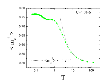
FIG. 1.: The temperature dependence of the local moment is shown at fixed $U=4$ for a 6x6 lattice. In addition to rising at $T\sim U$, as $T$ decreases, $m_{z}^{2}$ exhibits a second structure at lower temperature.

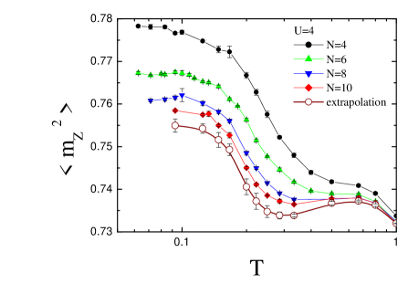
FIG. 2.: Data for the local moment for different lattice sizes. The low temperature feature in $m_{z}^{2}$ remains present as the lattice size is increased.

Additional insight is obtained by looking at the behavior of $m_{z}^{2}$ at different values of $U$, as in Fig. 3. The data of Fig. 3 are replotted in Fig. 4 to emphasize the universal nature of the high temperature behavior and the fact that the initial increase in the local moment as temperature is decreased does indeed occur at a temperature scale set by $U$.

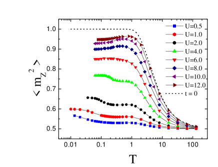
FIG. 3.: Temperature dependence of the local moment for different values of the on–site repulsion $U$ on 6x6 lattices. The dashed line corresponds to the zero-hopping limit, for $U=12$. The position of the low temperature feature first increases in temperature as $U$ increases, but then gradually falls, as emphasized later in Fig. 10.

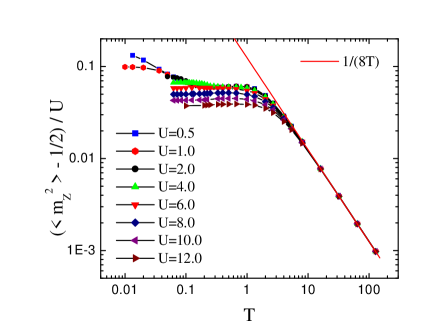
FIG. 4.: Scaled version of the data of Fig. 3. The plot shows that for high $T$ the local moment $m_{z}^{2}=\frac{1}{2}+{U\over 8T}$, that is, the deviation of the local moment from its noninteracting value $\frac{1}{2}$ exhibits a universal behavior with a temperature scale $U$.

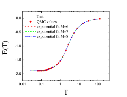
FIG. 5.: QMC values (circles) for the energy, and fittings provided by Eq. 5. Here $U=4$ and the lattice is 6x6. The different lines (dotted, dashed, dot-dashed) show that the fit is stable over a range of values of the number of fitting parameters.

In the zero-hopping ($t=0$) limit, $\langle m_{z}^{2}\rangle=1/\{{\rm exp}[-U/(2T)]+1\}$, which is monotonic with $T$, dropping from 1 at $T=0$ to 1/2 at $T\rightarrow\infty$. Why is the maximum in $\langle m_{z}^{2}\rangle$ shifted from $T=0$ when the hopping is present? The ground state is antiferromagnetic, with the effective exchange $J$ arising from virtual hopping of the electrons. This virtual transfer reduces the degree of localization as can be seen from the values of $\langle m_{z}^{2}\rangle$ at $T=0$ in Fig. 3. In the low-lying excited states the deviations from the antiferromagnetic state reduce the virtual hoppings since the Pauli principle forbids hopping when adjacent electron spins are ferromagnetically aligned. Localization is thereby increased with increasing temperature, giving rise to the maximum at $T\neq 0$. This maximum at large $U$ has also been observed in one-dimension.[8]

At weak coupling, we see the opposite effect. The local moment has instead an additional increase at low temperature. This has a natural explanation in terms of the formation of local magnetic order. If there is an energy gain with ordering, there will be an associated preference for large moments. It is interesting to note that the DMFT results[14] do not observe this additional moment enhancement at weak coupling. Instead, the local moment always has a maximum as a function of temperature. This is, perhaps, a consequence of restricting the DMFT to the paramagnetic phase.

B The Energy and Specific Heat

Figure 5 shows the QMC results for $E(T_{n})$ together with the exponential fit $E_{e}(T)$. Calculation of the specific heat brings out the low temperature features in $E(T)$. We begin our analysis of this data for the specific heat by looking at the data at relatively strong coupling ($U=10$) as shown in Fig. 6. It is seen that the results for the Hubbard model are beautifully fit by combining the zero-hopping $t=0$ specific heat, which lies right on the high $T$ Hubbard model results, and the Heisenberg specific heat,[32] which similarly lies right on the low $T$ Hubbard model results. The areas under both the low and high $T$ peaks are precisely $\ln{2}$, as expected for the high $T$ loss of entropy associated with moment formation and then low $T$ moment alignment. Clearly, this provides a good understanding of the strong coupling specific heat, as well as demonstrates the reliability of our approach to computing $C(T)$.

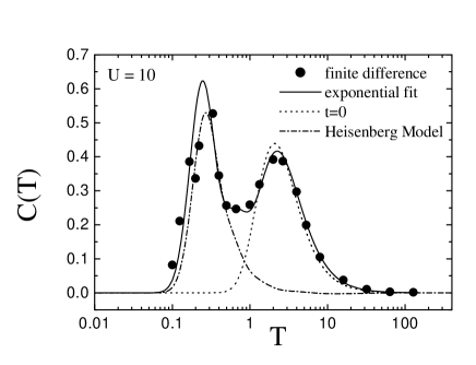
FIG. 6.: Results for the specific heat at $U=10$ and lattice size 6x6. The circles are numerical differentiation and the solid line is from the exponential fitting approach. The dotted line is the result for $C(T)$ at $t=0$ (that is, a single site). The dashed line is $C(T)$ for the Heisenberg model with $J=4t^{2}/U=0.4$.

Further confirmation of the accuracy of our $C(T)$ calculations is evident by comparing results for the numerical differentiation, the exponential fit, and the ME techniques as shown in Figs. 7 and 8. It is seen that the agreement between all three approaches is good. Figs. 7 and 8 also emphasize that both the exponential fit and ME techniques are well suited to capturing the two energy scales in the problem. It is also interesting to comment on the $U$ dependence of the areas under the specific heat curves of Fig. 6, 7, and 8. As $U$ decreases into the weak coupling regime, the low $T$ peak has less and less entropy. For $U=2$ the area is only about $\ln{2}/2$. This will be discussed at greater length shortly.

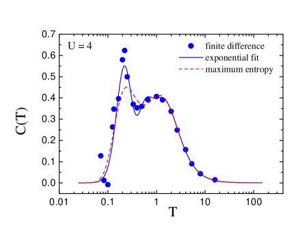
FIG. 7.: Results for the specific heat at $U=4$ and lattice size 6x6. The exponential fitting (full line) and ME results (dashed line) are in good agreement with direct numerical differentiation of the QMC data. Both smooth out the noise associated with direct numerical differentiation of the QMC data, though ME appears to broaden the results perhaps a bit too much.

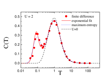
FIG. 8.: Results for the specific heat at $U=2$ and lattice size 6x6. The exponential fitting (full line) and ME results (dotted line) are both in good agreement with direct numerical differentiation of the QMC data. As at $U=4$, ME produces somewhat broader peaks. The dashed line is the specific heat for the non-interacting limit ($U=0$).

When the specific heat curves for different $U$ are plotted together, as in Fig. 9, one sees that there is a nearly universal crossing at high temperature. There has been considerable recent discussion of this phenomenon, both its occurrence in experimental systems like ³He and heavy fermion systems, and models like the Hubbard Hamiltonian.[14, 15, 16] In the case of the Hubbard model, the crossing has been argued to follow from the fact that the high temperature entropy is independent of $U$, ln4 = $\int_{0}^{\infty}C(T,U)dT/T,$ which implies that $0=\int_{0}^{\infty}\partial C/\partial UdT/T$. Hence $\partial C/\partial U$ must be positive for some temperature ranges and negative for others, a condition for crossing to occur.[15] The narrowness of the crossing region is traced ultimately to the linear temperature dependence of the double occupancy, the conjugate variable associated with $U$.[15] In DMFT, two crossings were observed for the Hubbard model, with the high temperature one being nearly universal, while the low temperature intersections were considerably more spread out.

Previous studies in two dimensions[3] exhibit crossings of the specific heat at $T_{*}=1.6$, with a crossing region $\Delta T_{*}=0.2$. In Fig. 9 we confirm this result that a specific heat crossing occurs in two dimensions. While the crossings in the earlier study[3] shift systematically with $U$, we instead see a random fluctuation of the crossing point. This suggests that the width of the crossing we report here is dominated by statistical fluctuations as opposed to possible systematic effects. We have also verified that the double occupancy has a linear temperature dependence at low $T$, especially at weak coupling, which is the criterion established for a universal crossing point.

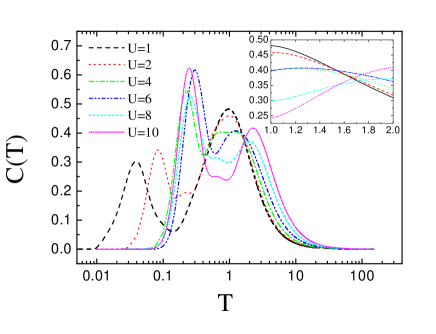
FIG. 9.: The specific heat curves for different $U$ values show a nearly universal high temperature crossing for the two dimensional Hubbard model, as has previously been observed in DMFT and in several experimental systems.

The position of the two peaks as a function of $U$ is shown in Fig. 10. The strong coupling analysis gives us firm predictions for the peak positions at large $U$: First, the $t=0$ result tells us that the high $T$ peak is at $T_{{\rm high}}\approx U/4.8$. The deviation from this limit seen in Fig. 10 can be ascribed to quantum fluctuations. Meanwhile, the Heisenberg result for the low $T$ peak is at $T_{{\rm low}}=2J/3=8t^{2}/3U$. [33] We similarly understand the position of $T_{{\rm high}}$ at weak coupling from the $U=0$ analysis: $T_{{\rm high}}\approx t=1$ in units where $t=1$. The value of $T_{{\rm low}}$ for weak coupling is somewhat more problematic. In three dimensions, the Neél temperature which describes the onset of long–range magnetic order, has a non–monotonic behavior with $U$,[4, 34] first rising[7] at small $U$ as $T_{N}\propto{\rm exp}[-2\pi t/U]$ and subsequently falling back down as $T_{N}\propto t^{2}/U$ at large $U$. In lower dimensions, like the 2–d case studied in this paper, $T_{N}=0$. Nevertheless, in weak coupling, both the random phase approximation[7] and Hartree-Fock calculations give a finite $T_{N}\propto{\rm exp}[-2\pi\sqrt{t/U}]$ in 2–d. It is tempting in this case to interpret this energy scale as that of the short range spin fluctuations which give rise to the low temperature peak in $C$ at weak coupling, and similarly $t^{2}/U$ as the corresponding energy scale at strong coupling. Indeed, both the increase for small $U$, consistent with the exponential form, and the subsequent decrease can be seen in $T_{{\rm low}}$ in Fig.  10. It might also be noted that the entropy in the low-$T$ Hartree-Fock $C(T)$ peak goes to $0$ as $U\rightarrow 0$, which is also consistent with the decreasing entropy under the low-$T$ QMC $C(T)$ peak as $U$ becomes small.[35]

Finite size effects are illustrated in Fig. 11, which shows the data for the specific heat, obtained by finite differention of the energy data, on 6x6 and 10x10 lattices at $U=2$. As is seen, the error bars as inferred from the scatter in the data are of the same size as any possible systematic effect. In determinant QMC, finite size effects are largest at weak coupling, so this data represents a rather stringent test of possible lattice size dependence of our results for the thermodynamics.

We now turn to the issue of the separate contributions of the kinetic $K$ and potential $P$ energies to the specific heat. As discussed in the introduction, we might associate the charge peak with the potential energy, since the energy $U$ is what enforces double occupancy and reduces charge fluctuations. Since the energy scale $J=4t^{2}/U$ arises from virtual hopping processes, it is more naturally associated with the kinetic energy. At strong coupling this division describes the mapping of the Hubbard model onto the Heisenberg model, and then the specific heat of the Heisenberg model itself, and works extremely well quantitatively, as seen in Fig. 6.

FIG. 10.: Position of the high $T$ and low $T$ peaks of the specific heat. The dotted line is the Heisenberg limt $T\sim 2J/3$, the full line corresponds to the $t=0$ limit, $T\sim U/4.8$ and the dash-dotted line corresponds to an RPA–like form for the temperature scale of the antiferromagnetic spin fluctuations, $T\sim{\rm exp}[-2\pi\sqrt{t/U}]$.

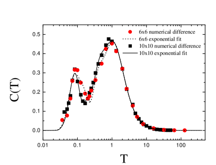
FIG. 11.: Comparison of results for the specific heat at $U=2$ and lattice sizes 6x6 and 10x10.

At intermediate coupling it is not so natural to consider separately the derivatives of the kinetic and potential energies, as these quantities mix dramatically. Indeed, the behavior of the local moment shown in Fig. 1 indicates that at $U=4$ the potential energy in fact contributes both to the low and high temperature structure of $C(T)$.

Figure 12 shows $dP/dT$ and $dK/dT$ for $U=2,4,10$. At strong coupling $U=10$, $dP/dT$ has a high temperature maximum, while $dK/dT$ has a low temperature peak, as expected. In the combined specific heat, then, $P$ and $K$ are responsible for the charge and spin peaks respectively. Interestingly, however, even at large $U$, $dP/dT$ has a significant negative dip at low $T$, reflecting the potential energy cost of delocalization. As we have remarked, this effect has previously been noted in the 1–d Hubbard model and DMFT.[8, 14]

The positions of the contributions of $dP/dT$ and $dK/dT$ to $C(T)$ are exchanged as $U$ is decreased. Finally, at $U=2$, it is the potential energy which is responsible for the low temperature ’spin’ peak, and the kinetic energy for the high temperature ’charge’ peak.

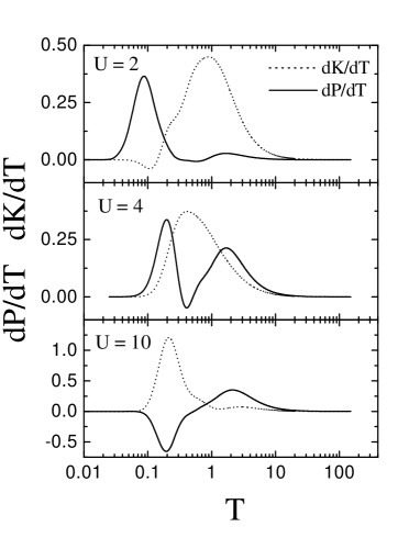
FIG. 12.: The separate temperature derivatives of the kinetic and potential energy. At strong coupling, the temperature dependence of the potential energy and kinetic energies give rise to the ’charge’ and spin peaks in $C$ respectively. This attribution is interchanged at weak coupling.

The entropy $S$ can also be obtained as the area under $(1/T)C(T)$, as well as the separate kinetic and potential contributions. Fig. 13 shows the results at $U=2$, $U=4$ and $U=10$. In all cases the value of $S$ at high temperature equals the expected $2\ln{2}$ to within a few percent. At strong coupling, $U=10$, the offsetting kinetic and potential contributions seen in the low-$T$ peak region in Fig. 12 are reflected as well in Fig. 13. Nevertheless, the total entropy (solid curve) shows a shoulder at $\ln{2}$ and then the final high-temperature value of $2\ln{2}$ reflecting the two peaks in Fig. 6, which correspond first to the “Heisenberg” disordering of the spins and then at higher temperature to the destruction of local moments. At weak coupling, the initial increase in entropy at low $T$ comes from the temperature dependence of the potential energy which, as we have seen, is what gives rise to the low $T$ peak in $C(T)$. The area under the low $T$ peak in $C(T)/T$ is reduced from its large $U$ value of $\ln{2}$. Certainly one origin of this decrease is the reduction of the local moment $m_{z}^{2}$ from its large $U$ value $m_{z}^{2}=1$ at small $U$, as seen in Fig. 3. The entropy associated with local ordering of moments scales with the moment size.[35]

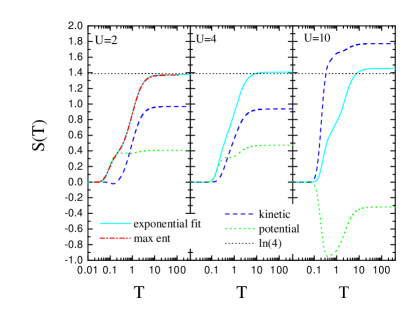
FIG. 13.: The temperature dependence of the entropy.

C Magnetic Correlations

It is natural to associate the low temperature feature in the local moment and therefore the low $T$ peak in $C(T)$ with the onset of local antiferromagnetic correlations between neighboring spins. To understand how these correlations develop we have calculated the spin-spin correlation function between neighboring sites $\langle S_{i}S_{{\bf i}+\hat{x}}\rangle$ and the magnetic structure factor $S({\bf Q})$. Figure 14 shows these two quantities as a function of temperature for $U=2$. The inset shows the derivatives of the spin-spin correlation function for neighboring sites ($dS_{\bf i}S_{{\bf i}+\hat{x}}/dT$) and for the magnetic structure factor ($dS({\bf Q})/dT$) with respect to the temperature: the sharp peaks form roughly at the same position as the specific heat has its low $T$ peak. Since $T_{N}=0$, the peak in $dS({\bf Q})/dT$ should not be associated with long ranged correlations. Indeed, the largest contribution to $dS({\bf Q})/dT$ comes from antiferromagnetic correlations between neighboring spins.

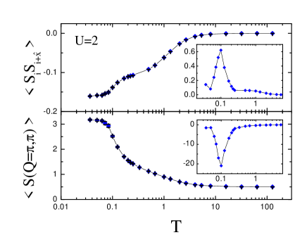
FIG. 14.: Spin-spin correlation between neighboring sites and magnetic structure factor as a function of temperature for a 6x6 lattice with $U=2$. The insets show the derivatives of these two quantities with temperature.

IV Density of States and Optical Conductivity

A The Density of States:

While the standard interpretation of the two peak structure in the specific heat in terms of the freezing out of charge and spin fluctuations, at high and low $T$ respectively, is consistent with our data at large $U$, Fig. 12 emphasized that such a picture is not as useful at weak coupling.

Greater insight into the physics behind the specific heat is obtained by looking at the dynamics. Figure 15 shows results for the density of states $N(\omega)$ for $U=1,2,4,6$ and decreasing temperatures. At high $T$ the density of states consists of a single, very broad, bump with maximum at $\omega=0$. As $T$ is lowered for the smaller $U$ values (e.g., $U=2$), $N(\omega=0)$ first increases as a quasiparticle peak develops at $\omega=0$. This peak appears to be very similar to that found in multiband models like the periodic Anderson model, where it is associated with a Kondo resonance. As $T$ is lowered yet further, $N(\omega)$ then begins to decrease as a dip begins to form in the center of the quasiparticle peak.

For larger $U$, on the other hand (e.g., $U=6$), only the dip develops with decreasing temperature, and so $N(\omega=0)$ always decreases as $T$ is lowered. This behavior is emphasized in Fig. 16 which shows $N(\omega=0)$ as a function of temperature for $U=2,4,6$. The temperature at which $N(\omega=0)$ becomes small is seen in Fig. 16 to increase with $U$, and it appears correlated with the position of the low $T$ peak in $C(T)$. Indeed, the derivative of $N(\omega=0)$ is maximum at the same temperature where $C(T)$ has its low $T$ peak (indicated by arrows in the plot).

This “pseudogap” in the density of states is one of the central features of the 2–d Hubbard model under recent discussion, since it is one of the most interesting features of the normal state of the high temperature superconductors in the underdoped regime.[36] As the pseudogap has a d–wave symmetry, like the superconducting order parameter itself, it is believed to arise as a result of short–range spin fluctuations which might also play a role in the pairing. The pseudogap’s existence has a long history of discussion, and debate, in the numerical literature on the Hubbard model which we shall now review, since concerns about possible finite size effects in the pseudogap may bear on similar concerns in the behavior of the specific heat.

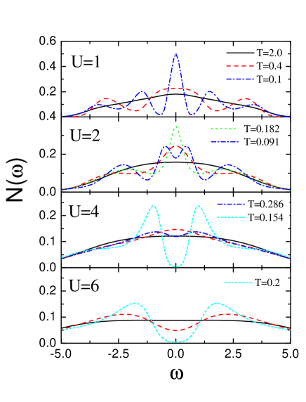
FIG. 15.: The temperature evolution of the density of states at $U=1,2,4,6$ on a 6x6 lattice. For $U=1,2$, as $T$ is lowered, the single broad peak first evolves into a sharper quasiparticle peak before a pseudogap opens. The quasiparticle peak is washed out as $U$ increases.

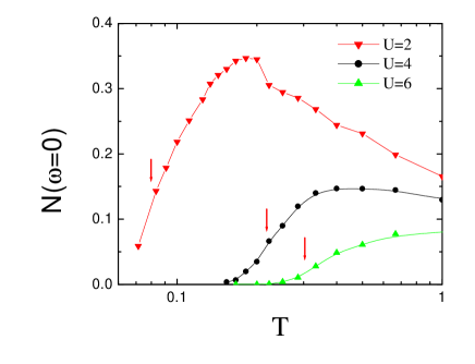
FIG. 16.: The zero frequency density of states at $U=2,4,6$ and 6x6 lattice. The arrows indicate the location of the low $T$ peaks in the specific heat.

The dynamical data presented in Figs. 15–16 do not make a fully compelling case for the relation between the low $T$ peak in $C(T)$ and the pseudogap, since they are for a single fixed lattice size. A particular issue is the behavior of the density of states $N(\omega)$ of the half–filled Hubbard model in the thermodynamic limit. Quantum Monte Carlo results concerning this question are still evolving. Early simulations had the somewhat surprising conclusion that a pseudogap in $N(\omega)$ was present at weak to intermediate coupling only at $T=0$ in the thermodynamic limit. That is, while on a fixed lattice size $L$ a gap in $N(\omega)$ develops at a finite temperature $T$, it would go away if the lattice size were increased.[31] Meanwhile, at strong coupling, the same work found the pseudogap persists at finite $T$ even as the system size increases. This behavior was interpreted as reflecting the fact that long range antiferromagnetic correlations are present only at $T=0$, and that such long range correlations were required for a gap in $N(\omega)$ for small $U$. This interpretation was questioned, however, since one might expect the pseudogap to depend only on the existence of short range antiferromagnetic correlations. Such local order should form at a temperature which is independent of lattice size, leading to the conclusion that the pseudogap should be present below that temperature even on large lattices.

If the original suggestion that the finite temperature pseudogap disappears at weak coupling in the thermodynamic limit were the case, it might raise similar questions about possible finite size effects in our results for the low temperature structure of the magnetic moment and specific heat. We believe this is not a concern for three reasons. First, one can consider the limit of very weak coupling. As we already see in Fig. 8, the high $T$ peak in $C(T)$ is well fit by a noninteracting calculation, and specifically therefore comes from the kinetic energy. If the local moment (potential energy) did not evolve at low $T$, then $C(T)$ would have a single peak structure. Therefore, our separate finite size scaling analysis for the moment and the specific heat support each other. Second, we have presented data at different finite sizes (Fig. 11) which show no evidence for the low $T$ peak shifting with increased lattice size. Finally, recent work suggests that the pseudogap exists in the thermodynamic limit at weak coupling and is not a finite size effect there.[37, 38, 39, 40]

B The Optical Conductivity

The density of states itself does not present a complete picture of the nature of the excitation gap. A more refined view may be obtained by looking at the optical conductivity, as shown in Figs. 17–19. These results show that the Hubbard model has a non–zero charge gap, even at weak to intermediate coupling where $U$ is less than the bandwidth. We examine the dynamic spin susceptibility (not shown) and find the spin gap to vanish since the 2–d Hubbard model has long range magnetic order at $T=0$ and hence ungapped, power law, spin wave excitations.

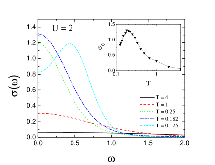
FIG. 17.: The frequency dependence of the optical conductivity for $U=2$ and different temperatures. Inset: The zero frequency value as a function of temperature, indicating the opening of a Mott gap.

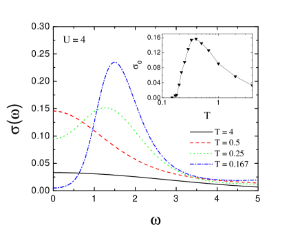
FIG. 18.: Same as Fig. 17 except $U=4$.

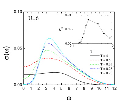
FIG. 19.: Same as Fig. 17 except $U=6$.

V Conclusions

In this paper we have examined carefully the low temperature structure of the local moment and specific heat of the two dimensional Hubbard model. A striking conclusion of our work is that the two peak structure in the specific heat is preserved down to $U=t=W/8$, where $W=8t$ is the bandwidth. In one dimension, the coalescence of the spin and charge peaks appears to occur at much larger $U$, namely the one dimensional bandwidth. Meanwhile, in infinite dimension, the peaks also come together at an interaction strength associated with an average kinetic energy per particle corresponding to half the two dimensional bandwidth. However, we have pointed out that the argument that the peaks come together which is based on a comparison of the scales $4t^{2}/U$ and $U$ might be flawed, as the weak coupling spin energy scale is instead set by $t\,{\rm exp}(-2\pi\sqrt{t/U})$. This leaves open the question of why the separation of the specific heat energy scales is maximal in intermediate dimension. Possibly the half-filled two-dimensional Hubbard model is unique due to the unusual characteristics of its noninteracting states at the Fermi energy.[6] However, it should also be recalled that the DMFT studies have been restricted to the paramagnetic phase, which may have an important impact on the existence of two well defined peaks. Finally the existence of the Nagaoka state in two dimensions, but not in one or infinite dimensions, indicates that there may be no reason to expect systematic behavior here as a function of dimension.[41]

We have emphasized that the standard nomenclature which identifies the high temperature peak in the specific heat as due to “charge” fluctuations and the low temperature peak as due to “spin” fluctuations while useful at strong coupling, needs to be refined. At weak coupling, the high temperature peak comes from the kinetic energy while the low temperature peak comes from the potential energy. By comparing with the behavior of the density of states, we have argued that the structure of $C(T)$ may be associated with “pseudogap” formation, that is, the onset of short range antiferromagnetic correlations between near–neighbor spins.

A detailed understanding of the relationship of the energy and local moment formation is desirable in a number of contexts in using model Hamiltonians to describe strongly correlated materials. In particular, while minimization of the energy determines the dominant low temperature phases, the various types of behavior of the local moment (for example screening by conduction electrons in multi–band models) can also provide important clues concerning the suitability of different models in describing the low temperature physics.[42]

- [1] See The Hubbard Model, A. Montorsi, ed, World Scientific (1992); The Hubbard Model–Recent Results M. Rasetti, ed, World Scientific (1991); and references therein.
- [2] M. Takahashi, Prog. Theor. Phys. 52, 103 (1974).
- [3] D. Duffy and A. Moreo, Phys. Rev. B 55, 12918 (1997).
- [4] R. T. Scalettar, D. J. Scalapino, R. L. Sugar, and D. Toussaint, Phys. Rev. B 39, 4711 (1989).
- [5] R. Staudt, M. Dzierzawa, and A. Muramatsu, unpublished, cond-mat/0007042.
- [6] J.E. Hirsch, Phys. Rev. B 31, 4403 (1985).
- [7] The weak coupling form of the Neél temperature comes from the random phase approximation condition , where is the noninteracting spin susceptibility, As emphasized by Hirsch, the simultaneous occurrence of nesting and a logarithmic van–Hove singularity in the density of states of the two–dimensional Hubbard model at half–filling introduces a square root in the exponential which describes the RPA form of the spin fluctuation energy scale.
- [8] H. Shiba and P. A. Pincus, Phys. Rev. B 5, 1966 (1972).
- [9] J. Schulte and M. Böhm, Phys. Rev. B 53, 15385 (1996).
- [10] T. Usuki, N. Kawakami, and A. Okiji, J. Phys. Soc. Jpn. 59, 1357 (1989).
- [11] T. Koma, Prog. Theor. Phys. 83, 655 (1990).
- [12] M. M. Sanchez, A. Avella, and F. Mancini, Europhys. Lett 44, 328 (1998).
- [13] G. Jütner, A. Klümper and J. Suzuki, Nucl. Phys B 522, 471 (1998).
- [14] A. Georges and W. Krauth, Phys. Rev. B48, 7167 (1993).
- [15] D. Vollhardt, Phys. Rev. Lett. 78, 1307 (1997).
- [16] N. Chandra, M. Kollar, and D. Vollhardt, Phys. Rev. B59, 10541 (1999).
- [17] We actually evaluate all three components of the local moment , , . They are, of course, equal.
- [18] M. Jarrell and J.E. Gubernatis, Phys. Rep. 269, 135 (1996).
- [19] R. Blankenbecler, R.L. Sugar, and D.J. Scalapino, Phys. Rev. D 24, 2278 (1981).
- [20] In classical Monte Carlo, the best approach to evaluate is often to use the fluctuation formula . This is not a useful way to proceed for determinant Quantum Monte Carlo because the square of the Hamiltonian involves products of six and eight fermion operators, and the associated expectation values have large fluctuations.
- [21] A. McMahan, C. Huscroft, R.T. Scalettar, and E.L. Pollock, J. of Computer–Aided Materials Design 5, 131 (1998).
- [22] C. Huscroft, R. Gass, and M. Jarrell, cond–mat/9906155.
- [23] P. H. Bevington, in Data Reduction and Error Analysis for the Physical Sciences, McGraw-Hill Inc. (1969).
- [24] At , the term arises from momenta states at the Fermi surface, i.e. with which do not contribute ln to the entropy. Such are a finite fraction of the total momentum values for calculations on finite clusters, but decrease in weight as the lattice size is increased. Similarly, within mean field theory, the Hamiltonian for finite can be diagonalized to give rise to single particle energy bands, and is again determined by the states at the Fermi surface. For the half–filled Hubbard model, in the paramagnetic phase, regardless of , the same states are at , and is fixed for a given periodic cluster size. For the antiferromagnetic phase the bands are split away from , and so . With an exact treatment of correlations, such as QMC provides, it is not a priori completely clear what the value of is. We found for the 2–d Hubbard model for our finite periodic clusters over a range of .
- [25] S.R. White, D.J. Scalapino, R.L. Sugar, E.Y. Loh, Jr., J.E. Gubernatis, and R.T. Scalettar, Phys. Rev. B 40, 506 (1989).
- [26] Our QMC data agree precisely with earlier work, which, however, did not go to quite so low temperatures and also used a more coarse temperature grid, and hence apparently did not detect the second low structure.
- [27] D. A. Huse, Phys. Rev. B 37, 2380 (1988).
- [28] A. Georges, G. Kotliar, W. Krauth, and M. Rozenberg, Rev. Mod. Phys. 68 13 (1996).
- [29] D. Vollhardt, in Correlated Electron Systems, V.J. Emery ed. (World Scientific, Singapore) 57 (1993); and Th. Pruschke, M. Jarrell, and J.K. Freericks, Adv. Phys. 44, 187 (1995).
- [30] M. Ulmke, R.T. Scalettar, A. Nazarenko, and E. Dagotto Phys. Rev. B54, 16523 (1996).
- [31] M. Vekic and S.R. White, Phys. Rev. B47, 1160 (1993).
- [32] The Heisenberg data were obtained with an independent code written with the world–line “loop algorithm”. See R.H. Swendsen and J.–S. Wang, Phys. Rev. Lett. 58, 86 (1987); N. Kawashima, J.E. Gubernatis, and H.G. Evertz, Phys. Rev. B50, 136 (1994); N.V. Prokofev, B.V. Svistunov, and I.S. Tupitsyn, JETP Lett. 64, 911 (1996); and B.B. Beard, and U.–J. Wiese, Phys. Rev. Lett. 77, 5130 (1997).
- [33] J. Jaklič and P. Prelovšek, Phys. Rev. Lett. 77, 892 (1996).
- [34] A.N. Tahvildar-Zadeh, J.K. Freericks, and M. Jarrell, Phys. Rev. B55, 942 (1997).
- [35] Even though the low peak in is not arising from long range magnetic order, the dependence of its area bears a resemblance to what happens at in a Hartree–Fock (HF) calculation. In HF, and in the thermodynamic limit, both paramagnetic and antiferromagnetic have the full area. The difference is that as is reduced below , the antiferromagnetic (AF) drops rapidly to zero, while the PM drops gradually to zero. In HF these are second order transitions, so is continuous, . But there is a discontinuity for the derivative, . So going up in from the AF stays 0 (AF gap) while the PM is larger and grows larger. Then just before the AF shoots up way above the PM , as first accesses the DOS to either side of the AF gap, followed by the discontinuity in dropping back to the PM value at . This has the appearance of a peak, which gets rounded off for finite sizes. Since and as it is clear that the area under this peak also goes to 0.
- [36] H. Ding, et al. Nature 382, 51 (1996); and F. Ronning et al., Science 282, 2067 (1998).
- [37] Y.M. Vilk and A.–M. S. Tremblay, J. Phys. I France 7, 1309 (1997).
- [38] S. Moukouri, S. Allen, F. Lemay, B. Kyung, D. Poulin, Y.M. Vilk and A.–M. S. Tremblay, cond–mat/9908053.
- [39] C. Huscroft, M. Jarrell, Th. Maier, S. Moukouri, and A.N. Tahvildarzadeh, cond–mat/9910226.
- [40] It is believed that the origin of the disagreement might be that the early data at small and large lattices had statistical errors which were big enough to cause problems in the analytic continuation. A. Tremblay, private communication.
- [41] P. Schlottmann, private communication
- [42] K. Held, C. Huscroft, R.T. Scalettar, and A. K. McMahan, Phys. Rev. Lett. 85, 373 (2000).