Superconductive properties of thin dirty SN bilayers

Abstract

The theory of superconductivity in thin SN sandwiches (bilayers) in the diffusive limit is developed within the standard Usadel equation method, with particular emphasis on the case of very thin superconductive layers, $d_{S}\ll d_{N}$. The proximity effect in the system is governed by the interlayer interface resistance (per channel) $\rho_{\rm int}$. The case of relatively low resistance (which can still have large absolute values) can be completely studied analytically. The theory describing the bilayer in this limit is of BCS type but with the minigap (in the single-particle density of states) $E_{g}\ll\Delta$ substituting the order parameter $\Delta$ in the standard BCS relations; the original relations are thus severely violated. In the opposite limit of an opaque interface, the behavior of the system is in many respects close to the BCS predictions. Over the entire range of $\rho_{\rm int}$, the properties of the bilayer are found numerically. Finally, it is shown that the results obtained for the bilayer also apply to more complicated structures such as SNS and NSN trilayers, SNINS and NSISN systems, and SN superlattices.

I Introduction

It is well known that the majority of metallic superconductors is well described by the classical BCS theory of superconductivity. [1] One of the main qualitative features of the BCS theory is a simple relation between the superconductive transition temperature $T_{c}$ and the low-temperature value of the energy gap for $s$-wave superconductors: $\Delta(0)=1.76\,T_{c}$. Experimentally, violations of this simple relation are considered as a sign of some unusual pairing symmetry or even of a non-BCS pairing mechanism; many theories of unconventional superconductivity were developed during the last decade, mainly in relation with high-$T_{c}$ materials. Recently, an evident example of such a violation of the BCS theory predictions was found in experiments by Kasumov et al., [2] who studied current-voltage characteristics of a carbon nanotube contact between two metallic bilayers (sandwiches) made of ordinary metals, tantalum and gold. The observed value of the low-temperature Josephson critical current is 40 times larger than the maximum expected (Ambegaokar-Baratoff) value [3] $I_{c}=\pi\Delta(0)/2eR_{\rm tube}$, where the energy gap of the bilayer $\Delta(0)$ is estimated from its transition temperature. The source of such discrepancy is not clear at present. The most recent experiments [4] demonstrate the existence of intrinsic superconductivity in carbon nanotubes. However, the discrepancy could be due to unusual superconductive properties of the bilayers. The aim of the present paper is to investigate these properties.

An essential feature of the experiment [[2]] was that the superconductive layer in the bilayer was very thin ($d_{S}/d_{N}$ = 5 nm/100 nm = 1/20). In the present paper, we investigate such a bilayer both analytically and numerically, calculating quantities characterizing the superconductivity in this proximity system: the order parameter $\Delta$, the density of the superconducting electrons $n$, the critical temperature $T_{c}$, the (mini)gap $E_{g}$ in the single-particle density of states (DOS) and the DOS $\nu(E)$ itself, the critical magnetic field $H_{c}$ parallel to the bilayer and the upper critical field $H_{c2}$ perpendicular to the bilayer. In our calculations, the parameter controlling the strength of the proximity effect is the (dimensionless) resistance of the SN interface per channel $\rho_{\rm int}$, which is related to the total interface resistance $R_{\rm int}$ as

$$R_{\rm int}=\frac{R_{q}\rho_{\rm int}}{2N_{\rm ch}},$$ (1)

where $R_{q}=h/e^{2}$ is the quantum resistance, and $N_{\rm ch}={\cal A}/(\lambda_{F}/2)^{2}$, with $\lambda_{F}$ being the Fermi wave-length, is the number of channels in the interface of area ${\cal A}$. We choose $\lambda_{F}$ referring to the S layer.

Our results show that the values of the interface resistance can be divided into three ranges: (a) at large resistance, many characteristics of the superconductor [$\Delta$, $n$, $T_{c}$, $\nu(E)$, $H_{c}$, $H_{c2}$] are almost unaffected by the presence of the normal layer, i.e., this is the BCS limit (however, we note that $E_{g}$ does not coincide with the order parameter, and even vanishes as $\rho_{\rm int}$ increases); (b) at low resistance, the theory describing the bilayer is of BCS type but with the order parameter $\Delta$ substituted by the minigap $E_{g}$ (for instance, $E_{g}=1.76\,T_{c}$, whereas $E_{g}\ll\Delta$); the original BCS relations are thus severely violated; (c) at intermediate resistance, the behavior of the system interpolates between the above two regimes.

The paper is organized as follows. In Section II, we formulate the standard technique of the Usadel equations for dirty systems, [5] and introduce a convenient angular parameterization of the quasiclassical Green functions entering these equations. In Section III, we apply the Usadel equations to the thin bilayer that we intend to discuss, and present numerical results for $\Delta$, $n$, $T_{c}$, and $\nu(E)$. We start an analytical analysis of the Usadel equations for the bilayer by calculating the minigap $E_{g}$ in the density of states in the two limiting cases of high and low interface resistance (Section IV). Then, in Section V, we elucidate the structure of the theory describing the system in the so-called Anderson limit (of relatively low resistance), finding $\Delta$, $n$, $T_{c}$, $E_{g}$, and $\nu(E)$. The critical magnetic fields $H_{c}$ (parallel to the bilayer) and $H_{c2}$ (perpendicular to the bilayer) are calculated in Sections VI and VII, respectively. In Section VIII, we show that the results obtained for the bilayer also apply to more complicated structures such as SNS and NSN trilayers, SNINS and NSISN systems, and SN superlattices. The relationship between our results and the experiment [[2]] that has stimulated our research is discussed in Section IX. Finally, we present our conclusions (Section X).

II Method

A Usadel equation

Equilibrium properties of dirty systems are described [6] by the quasiclassical retarded Green function $\hat{R}({\bf r},E)$, which is a $2\times 2$ matrix in the Nambu space satisfying the normalization condition $\hat{R}^{2}=\hat{1}$. The retarded Green function obeys the Usadel equation

$$D\nabla(\hat{R}\nabla\hat{R})+i[\hat{H},\,\hat{R}]=0.$$ (2)

Here the square brackets denote the commutator, $D={\rm v}l/3$ is the diffusion constant with ${\rm v}$ and $l$ being the Fermi velocity and the elastic mean free path, $\hat{H}=E\hat{\sigma}_{z}+\hat{\Delta}({\bf r})$ with $E$ being the energy, whereas $\hat{\sigma}_{z}$ (the Pauli matrix) and $\hat{\Delta}({\bf r})$ are given by

$$\hat{\sigma}_{z}=\left(\begin{array}[]{cc}1&0\\ 0&-1\end{array}\right),\qquad\hat{\Delta}=\left(\begin{array}[]{cc}0&\Delta\\ -\Delta^{*}&0\end{array}\right).$$ (3)

The order parameter $\Delta({\bf r})$ must be determined self-consistently from the equation

$$\hat{\Delta}({\bf r})=\frac{\nu_{0}\lambda}{4}\!\int_{0}^{\omega_{D}}\!\!\!dE\,\tanh\!\left(\!\frac{E}{2T}\!\right)\!\left[\hat{R}({\bf r},E)-\hat{R}({\bf r},-E)\right]_{\rm o.d.},$$ (4)

where the subscript $\rm o.d.$ denotes the off-diagonal part, $\nu_{0}=m^{2}{\rm v}/\pi^{2}$ is the normal-metal density of states at the Fermi level, $\lambda$ is the effective constant of electron-electron interaction in the S layer (whereas we assume $\lambda=0$ and hence $\Delta=0$ in the N layer), and integration is cut off at the Debye energy $\omega_{D}$ of the S material.

Equation (2) should be supplemented with the appropriate boundary conditions at an interface, which read [7]

$$\sigma_{l}\left(\hat{R}_{l}\nabla_{\bf n}\hat{R}_{l}\right)=\sigma_{r}\left(\hat{R}_{r}\nabla_{\bf n}\hat{R}_{r}\right)=\frac{g_{\rm int}}{2}\left[\hat{R}_{l},\,\hat{R}_{r}\right],$$ (5)

where the subscripts $l$ and $r$ designate the left and right electrode, respectively; $\sigma$ is the conductivity of a metal in the normal state, and $g_{\rm int}=G_{\rm int}/{\cal A}$ (with $G_{\rm int}=1/R_{\rm int}$) is the conductance of the interface per unit area when both left and right electrodes are in the normal state. $\nabla_{\bf n}$ denotes the projection of the gradient upon the unit vector ${\bf n}$ normal to the interface.

The system of units in which the Planck constant and the speed of light equal unity ($\hbar=c=1$) is used throughout the paper.

B Angular parameterization of the Green function

The normalization condition allows the angular parameterization of the retarded Green function:

$$\hat{R}=\left(\begin{array}[]{cc}\cos\theta&-ie^{i\varphi}\sin\theta\\ ie^{-i\varphi}\sin\theta&-\cos\theta\end{array}\right),$$ (6)

where $\theta=\theta({\bf r},E)$ is a complex angle which characterizes the pairing, and $\varphi=\varphi({\bf r},E)$ is the real superconducting phase. The off-diagonal elements of the matrix $\hat{R}$ describe [6] the superconductive correlations, vanishing in the bulk of a normal metal ($\theta=0$).

The Usadel equation takes the form

$$\frac{D}{2}\nabla^{2}\theta+\left[iE-\frac{D}{2}\left(\nabla\varphi\right)^{2}\cos\theta\right]\sin\theta+\left|\Delta\right|\cos\theta=0,$$ (8)

$$\nabla\left(\sin^{2}\theta\,\nabla\varphi\right)=0.$$ (9)

The corresponding boundary conditions are

$$\sigma_{l}\nabla_{\bf n}\theta_{l}=g_{\rm int}\left[\cos(\varphi_{r}-\varphi_{l})\cos\theta_{l}\sin\theta_{r}-\sin\theta_{l}\cos\theta_{r}\right],$$ (11)

$$\sigma_{r}\nabla_{\bf n}\theta_{r}=g_{\rm int}\left[\cos\theta_{l}\sin\theta_{r}-\cos(\varphi_{r}-\varphi_{l})\sin\theta_{l}\cos\theta_{r}\right],$$ (12)

$$\sigma_{l}\sin^{2}\theta_{l}\,\nabla_{\bf n}\varphi_{l} = \sigma_{r}\sin^{2}\theta_{r}\,\nabla_{\bf n}\varphi_{r}$$ (13)

$$= g_{\rm int}\sin(\varphi_{r}-\varphi_{l})\sin\theta_{l}\sin\theta_{r}.$$ (14)

The self-consistency equation for the order parameter $\Delta({\bf r})$ takes the form

$$\Delta=\frac{\nu_{0}\lambda}{2}\int_{0}^{\omega_{D}}dE\,\tanh\!\left(\!\frac{E}{2T}\!\right)\mathop{\rm Im}\nolimits\left[\sin\theta\right]e^{i\varphi}.$$ (15)

The above equations are written in the absence of an external magnetic field. To take account of the magnetic field, it is sufficient to substitute the superconducting phase gradient in the Usadel equations (II B) by its gauge invariant form $2m{\bf v}=\nabla\varphi+2e{\bf A}$, where ${\bf A}$ is the vector potential and ${\bf v}$ denotes the supercurrent velocity.

Physical properties of the system can be expressed in terms of the pairing angle $\theta({\bf r},E)$. The single-particle density of states $\nu({\bf r},E)$ and the density of the superconducting electrons $n({\bf r})$ are given by

$$\nu = \nu_{0}\mathop{\rm Re}\nolimits\,[\cos\theta],$$ (16)

$$n = \frac{2m\sigma}{e^{2}}\int_{0}^{\infty}dE\,\tanh\!\left(\!\frac{E}{2T}\!\right)\mathop{\rm Im}\nolimits\left[\sin^{2}\theta\right],$$ (17)

where $m$ and $e$ are the electron’s mass and the absolute value of its charge. The total number of single-particle states in a metal is the same in the superconducting and normal states, which is expressed by the constraint

$$\int_{0}^{\infty}dE\left[\nu({\bf r},E)-\nu_{0}\right]=0.$$ (18)

C Simple example: the BCS case

The simplest illustration for the above technique is the BCS case, when the order parameter $\Delta({\bf r})=\Delta_{BCS}$ is spatially constant. Its phase can be set equal to zero, $\varphi=0$. Then the Usadel equations (II B) are trivially solved, and we can write the answer in terms of the sine and the cosine of the pairing angle:

$$\sin\theta_{BCS}(E) = \frac{i\Delta_{BCS}}{\sqrt{E^{2}-\Delta_{BCS}^{2}}},$$ (20)

$$\cos\theta_{BCS}(E) = \frac{E}{\sqrt{E^{2}-\Delta_{BCS}^{2}}}.$$ (21)

An infinitesimal term $i0$ should be added to the energy $E$ to take the retarded nature of the Green function $\hat{R}$ into account, which yields

$$\mathop{\rm Im}\nolimits\left[\sin^{2}\theta_{BCS}(E)\right]=\frac{\pi}{2}\Delta_{BCS}\,\delta(E-\Delta_{BCS}).$$ (22)

The usual BCS relations are straightforwardly obtained from Eqs. (15), (16), (17) (for simplicity, we consider the case of zero temperature):

$$\Delta_{BCS} = 2\omega_{D}\exp\left(-\frac{2}{\nu_{0}\lambda}\right),$$ (23)

$$\nu_{BCS}(E) = \left\{\begin{array}[]{ll}\displaystyle 0,&\;\mbox{if }E<\Delta_{BCS}\\ \displaystyle\nu_{0}\frac{E}{\sqrt{E^{2}-\Delta_{BCS}^{2}}},&\;\mbox{if }E>\Delta_{BCS}\end{array}\right.,$$ (26)

$$n_{BCS} = \pi\frac{m\sigma}{e^{2}}\Delta_{BCS}.$$ (27)

The critical temperature must be determined from Eq. (15) with vanishing $\Delta(T_{c})$; the result is

$$\Delta_{BCS}(0)=\frac{\pi}{\gamma}T_{c}^{BCS},$$ (28)

where $\gamma\approx 1.78$ is Euler’s constant.

III Usadel equations for a thin bilayer

Let us consider a SN bilayer consisting of a normal metal ($-d_{N}<z<0$) in contact (at $z=0$) with a superconductor ($0<z<d_{S}$). We assume that the layers are thin (this assumption will be discussed in Sec. IX) and can be regarded as uniform, which allows us to set the order parameter $\Delta$ equal to a constant in the superconductive layer (we choose its phase $\varphi$ equal to zero). At the same time, we suppose that electron-electron interaction is absent in the normal layer: $\lambda=0$, hence $\Delta=0$, although the superconductive correlations ($\theta\neq 0$) exist in the N layer due to the proximity effect. The Usadel equations (II B) take the form

$$\frac{D_{N}}{2}\frac{\partial^{2}\theta_{N}}{\partial z^{2}}+iE\sin\theta_{N} = 0,$$ (30)

$$\frac{D_{S}}{2}\frac{\partial^{2}\theta_{S}}{\partial z^{2}}+iE\sin\theta_{S}+\Delta\cos\theta_{S} = 0,$$ (31)

where $\theta_{N}$ and $\theta_{S}$ denote the pairing angle $\theta$ at $z<0$ and $z>0$, respectively.

The boundary conditions (9) reduce to

$$\sigma_{N}\frac{\partial\theta_{N}}{\partial z}=\sigma_{S}\frac{\partial\theta_{S}}{\partial z}=g_{\rm int}\sin(\theta_{S}-\theta_{N}).$$ (32)

Equations (III) can be integrated once, yielding

$$\frac{D_{N}}{4}\left(\frac{\partial\theta_{N}}{\partial z}\right)^{2}-iE\cos\theta_{N} = f_{N},$$ (34)

$$\frac{D_{S}}{4}\left(\frac{\partial\theta_{S}}{\partial z}\right)^{2}-iE\cos\theta_{S}+\Delta\sin\theta_{S} = f_{S}.$$ (35)

The functions $f_{N}(E)$ and $f_{S}(E)$ are determined from the boundary condition $\partial\theta/\partial z=0$ at the nontransparent outer surfaces of the bilayer, which give

$$f_{N}(E) = -iE\cos\theta_{N}(-d_{N},E),$$ (36)

$$f_{S}(E) = -iE\cos\theta_{S}(d_{S},E)+\Delta\sin\theta_{S}(d_{S},E).$$ (37)

Let us denote $\theta_{N}(E)=\theta_{N}(-d_{N},E)$, $\theta_{S}(E)=\theta_{S}(d_{S},E)$. Because of the uniformity of the layers, the functions $\theta_{N}(z,E)$ and $\theta_{S}(z,E)$ are nearly spatially constant. However, in order to determine them, we should take account of their weak spatial dependence and make use of the boundary conditions at the SN interface. Substituting

$$\theta_{N}(z,E) = \theta_{N}(E)+\delta\theta_{N}(z,E),$$ (38)

$$\theta_{S}(z,E) = \theta_{S}(E)+\delta\theta_{S}(z,E)$$ (39)

into Eqs. (III) and linearizing them with respect to $|\delta\theta_{N}(z,E)|$, $|\delta\theta_{S}(z,E)|\ll 1$, we find the solution. Finally, boundary conditions at the SN interface lead to

$$-i\tau_{N}E\sin\theta_{N}(E) = i\tau_{S}E\sin\theta_{S}(E)+\tau_{S}\Delta\cos\theta_{S}(E)$$ (40)

$$= \sin\left[\theta_{S}(E)-\theta_{N}(E)\right],$$ (41)

where we have denoted $\tau_{N}=2\sigma_{N}d_{N}/D_{N}\,g_{\rm int}$, $\tau_{S}=2\sigma_{S}d_{S}/D_{S}\,g_{\rm int}$. Using the definition of the interface resistance per channel (1), we can represent these quantities as

$$\tau_{N}=2\pi\frac{{\rm v}_{N}d_{N}}{{\rm v}_{S}^{2}}\rho_{\rm int},\qquad\tau_{S}=2\pi\frac{d_{S}}{{\rm v}_{S}}\rho_{\rm int},$$ (42)

with ${\rm v}_{N}$ and ${\rm v}_{S}$ being the Fermi velocities in the N and S layers. The ratio $\tau_{N}/\tau_{S}={\rm v}_{N}d_{N}/{\rm v}_{S}d_{S}$, which is independent of interface properties, can also be interpreted as the ratio of the global densities of states (per energy interval) in the two layers considered,

$$\frac{\tau_{N}}{\tau_{S}}=\frac{{\cal A}d_{N}\nu_{0N}}{{\cal A}d_{S}\nu_{0S}}.$$ (43)

The latter interpretation will prove useful for further analysis.

Having solved the boundary conditions (40), we can determine all equilibrium properties of the system (because knowledge of $\theta_{S}$, $\theta_{N}$ implies knowledge of the retarded Green function $\hat{R}$).

A useful representation of the boundary conditions (40) is obtained as follows. Excluding $\theta_{N}(E)$ from Eq. (40), we arrive at a single equation for the function $\theta_{S}(E)$, which can be written, in terms of $Z=\exp(i\theta_{S})$, as a polynomial equation

$$iC_{6}Z^{6}+C_{5}Z^{5}+iC_{4}Z^{4}+C_{3}Z^{3}+iC_{2}Z^{2}+C_{1}Z+iC_{0}$$ (45)

$$=0$$

with real coefficients

$$C_{6} = -\tau_{N}E\left(\frac{\tau_{S}}{\tau_{N}}\right)^{2}\left[1+\frac{\Delta}{E}\right]^{2},$$ (46)

$$C_{5} = \left[1-\left(\tau_{N}E\right)^{2}\right]\left(\frac{\tau_{S}}{\tau_{N}}\right)^{2}\left[1+\frac{\Delta}{E}\right]^{2}-1,$$ (47)

$$C_{4} = -\tau_{N}E\left(\frac{\tau_{S}}{\tau_{N}}\right)^{2}\left[3\left(\frac{\Delta}{E}\right)^{2}+2\frac{\Delta}{E}-1\right],$$ (48)

$$C_{3} = 2-2\left[1-\left(\tau_{N}E\right)^{2}\right]\left(\frac{\tau_{S}}{\tau_{N}}\right)^{2}\left[1-\left(\frac{\Delta}{E}\right)^{2}\right],$$ (49)

$$C_{2} = -\tau_{N}E\left(\frac{\tau_{S}}{\tau_{N}}\right)^{2}\left[3\left(\frac{\Delta}{E}\right)^{2}-2\frac{\Delta}{E}-1\right],$$ (50)

$$C_{1} = \left[1-\left(\tau_{N}E\right)^{2}\right]\left(\frac{\tau_{S}}{\tau_{N}}\right)^{2}\left[1-\frac{\Delta}{E}\right]^{2}-1,$$ (51)

$$C_{0} = -\tau_{N}E\left(\frac{\tau_{S}}{\tau_{N}}\right)^{2}\left[1-\frac{\Delta}{E}\right]^{2}.$$ (52)

During further analysis, the choice between the boundary conditions in the forms (40) and (45) will be a matter of convenience.

A Critical temperature

The critical temperature of the bilayer $T_{c}$ is defined from the condition of vanishing of the order parameter $\Delta$. Near $T_{c}$, the superconducting correlations are very small, $|\theta|\ll 1$; nevertheless, the self-consistency equation (15) has a nonzero solution $\Delta\neq 0$.

Linearizing the boundary conditions (40) with respect to $\theta_{N}$ and $\theta_{S}$, we readily find the solution:

$$\theta_{S}(E)=i\frac{\Delta}{E}\left(1-\frac{\tau_{N}}{\tau_{S}+\tau_{N}-i\tau_{S}\tau_{N}E}\right).$$ (53)

Substituting this into the self-consistency equation (15) and simplifying both its sides by $\Delta$, we obtain an equation determining $T_{c}$, which can be cast into the form

$$\ln\frac{T_{c}^{BCS}}{T_{c}}=\frac{\tau_{N}}{\tau_{S}+\tau_{N}}\left[\vphantom{\sqrt{\left(\frac{\tau_{S}+\tau_{N}}{\tau_{S}\tau_{N}\omega_{D}}\right)^{2}}}\right. \psi\left(\frac{1}{2}+\frac{\tau_{S}+\tau_{N}}{2\pi T_{c}\tau_{S}\tau_{N}}\right)-\psi\left(\frac{1}{2}\right)$$ (55)

$$\left.-\ln\sqrt{1+\left(\frac{\tau_{S}+\tau_{N}}{\tau_{S}\tau_{N}\omega_{D}}\right)^{2}}\right],$$

where $\psi(x)$ denotes the digamma function. A similar formula (except the logarithmic term in the r.h.s.) was obtained by McMillan [8, 9, 10] (see also Ref. [[11]]). The logarithmic term in the r.h.s. takes account of the finiteness of the Debye energy $\omega_{D}$; it becomes important only in the limit of a perfect interface (the Cooper limit), i.e., when $\tau_{S}\tau_{N}\omega_{D}/(\tau_{S}+\tau_{N})\ll 1$. Equation (55) can be solved numerically over the entire range of $\rho_{\rm int}$ (see Sec. III B); the analytical solution can be found in limiting cases (see Sec. V).

B Numerical results

The solution of Eq. (45) can be found numerically. To this end, we solve the system of two nonlinear equations for the functions $\mathop{\rm Re}\nolimits Z(E)$ and $\mathop{\rm Im}\nolimits Z(E)$, using the modified Newton method with normalization.

The solution depends on the bilayer’s parameters: the thicknesses of the layers, characteristics of materials constituting the bilayer, and the quality of the SN interface. This dependence enters Eqs. (45), (52) via $\tau_{N}$ and $\tau_{S}$. For numerical calculations, we assume the characteristics of the bilayer to be the same as in the experiment by Kasumov et al. [2] The superconductive layer is made of tantalum, $d_{S}=5$ nm, and the normal layer is made of gold, $d_{N}=100$ nm. Approximate experimental values of the conductivities are [12] $\sigma_{S}=0.01\,\mu\Omega^{-1}\,{\rm cm}^{-1}$ and $\sigma_{N}=1\,\mu\Omega^{-1}\,{\rm cm}^{-1}$. In order to calculate the Fermi characteristics of tantalum and gold, we use the values of the Fermi energy $E_{F}({\rm Ta})=11$ eV, $E_{F}({\rm Au})=5.5$ eV, and the free electrons model. [13]

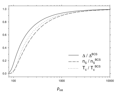
FIG. 1.: Dependence of the order parameter in the S layer $\Delta$, of the superconducting electrons’ density in the S layer $n_{S}$, and of the bilayer’s critical temperature $T_{c}$ on the interface resistance per channel $\rho_{\rm int}$ at zero temperature. All the quantities are normalized by the corresponding BCS values. The discrepancy between the curves implies a violation of the BCS relations between $\Delta$, $n_{S}$, and $T_{c}$.

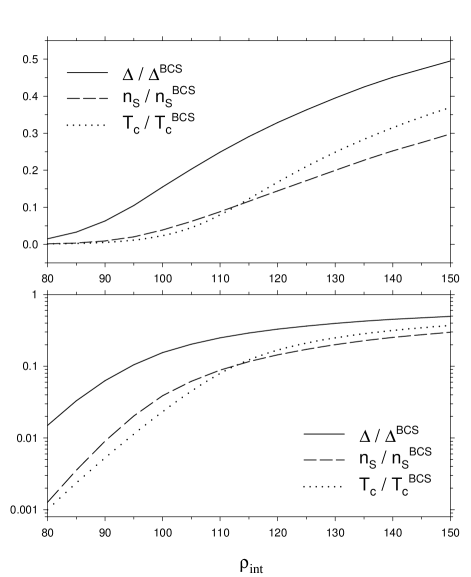
FIG. 2.: Zoomed part of Fig. 1. In the shown range of relatively small resistance $\rho_{\rm int}$, the BCS relations between $\Delta$, $n_{S}$, and $T_{c}$ are severely violated. The upper and lower graphs differ only in the scaling of the ordinate axis (normal and logarithmic, respectively).

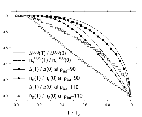
FIG. 3.: Temperature dependence of $\Delta$ and $n_{S}$ at $\rho_{\rm int}=$ 90 and 110. The temperature is normalized by the critical value $T_{c}$, which depends on $\rho_{\rm int}$; $\Delta$ and $n_{S}$ are normalized by their zero-temperature values. For comparison, the same dependence is also plotted for the BCS case.

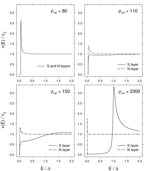
FIG. 4.: Energy dependence of the single-particle DOS, normalized by the normal-metal DOS, $\nu(E)/\nu_{0}$, in the S and N layers at $\rho_{\rm int}=$ 80, 110, 150, and 2000. The energy $E$ is normalized by the order parameter $\Delta$, which is different in all the four cases. [To avoid confusion, we note that actual (in absolute units) relation between the minigaps in the DOS does not correspond to what is seen from the Figure.] The Figure demonstrates drastic difference of the DOS in the bilayer from the BCS case [Eq. (26)].

Once the parameters have been specified, the solution of Eq. (45) depends only on the interface resistance $\rho_{\rm int}$. Having found the function $Z(E)$ [which is equivalent to finding $\theta_{S}(E)$], we start from the case of zero temperature, $T=0$, and study the dependence of the order parameter $\Delta$ and of the superconducting electrons’ density in the S layer $n_{S}$ [Eqs. (15), (17)] on $\rho_{\rm int}$. The results are plotted in Fig. 1, where we also show the dependence of the critical temperature $T_{c}$, determined from Eq. (55), on $\rho_{\rm int}$.

The suppression of $\Delta$, $n_{S}$, and $T_{c}$, in comparison to their BCS values in the S layer, is a natural consequence of proximity to the normal metal. At the same time, there is a possibility of BCS-like behavior, which implies the BCS relations between the suppressed quantities and the coincidence of the three curves plotted in Fig. 1. However, the curves split, and the difference between them is largest for relatively small values of $\rho_{\rm int}$. Figure 2 presents the range $80<\rho_{\rm int}<150$ on a larger scale.

Figure 3 shows the temperature dependence of the order parameter $\Delta$ and of the superconducting electrons’ density in the S layer $n_{S}$. Although the smaller $\rho_{\rm int}$ the further it is from the BCS limit (corresponding to $\rho_{\rm int}\to\infty$), we observe that at $\rho_{\rm int}=90$ the curves are closer to the BCS behavior than at $\rho_{\rm int}=110$. An explanation of this feature is given in Sec. V.

Finally, the energy dependence of the single-particle density of states in the S and N layers $\nu_{S,N}(E)$ is plotted in Fig. 4. The density of states in the bilayer is qualitatively different from the BCS result (26). In particular, there is a minigap $E_{g}$ in the density of states at energies much smaller then $\Delta_{BCS}$, and even much smaller then $\Delta$ in the bilayer. In the next Section, we find this minigap analytically in the two limiting cases of small and large interface resistance $\rho_{\rm int}$. Another feature which can be seen from Fig. 4 is that the order parameter $\Delta$ plays the role of a characteristic energy scale of the system only in the limit of large $\rho_{\rm int}$ (see the case $\rho_{\rm int}=2000$). Otherwise, no peculiarity in the DOS is observed at $E=\Delta$. Some other aspects of the DOS behavior will be discussed in Secs. IV, V.

IV Minigap in the density of states

In principle, the energy dependence of the single-particle density of states is different in the S and N layers. At the same time, the gap in the DOS is a property of the bilayer as a whole; the gap is spatially independent because there is no localization in the system and each electronic state extends over the whole bilayer.

The presence of the gap thus implies that the density of states vanishes in both layers, when the energy is below the gap:

$$\mathop{\rm Re}\nolimits\,[\cos\theta_{S}]=\mathop{\rm Re}\nolimits\,[\cos\theta_{N}]=0,$$ (56)

leading to $\theta_{S}=\frac{\pi}{2}+i\vartheta_{S}$, $\theta_{N}=\frac{\pi}{2}+i\vartheta_{N}$, with real $\vartheta_{S}$ and $\vartheta_{N}$. In this case, Eqs. (40) can be written as

$$\tanh\vartheta_{N} = \frac{\sinh\vartheta_{S}+\tau_{N}E}{\cosh\vartheta_{S}},$$ (58)

$$\cosh\vartheta_{N} = -\frac{\tau_{S}}{\tau_{N}}\cosh\vartheta_{S}+\frac{\tau_{S}\Delta}{\tau_{N}E}\sinh\vartheta_{S}.$$ (59)

Assuming that $\sinh\vartheta_{S}\gg\tau_{N}E$ at small energies, from Eqs. (56) we obtain $\vartheta_{N}=\vartheta_{S}$, and, finally,

$$\cos\theta_{S}=\cos\theta_{N}=\frac{E}{\sqrt{E^{2}-E_{g}^{2}}},$$ (60)

with $E_{g}=\tau_{S}\Delta/(\tau_{S}+\tau_{N})$. This is a BCS-like result [cf. Eq. (21)], although the order parameter $\Delta_{BCS}$ is substituted by the minigap $E_{g}$. The assumption is readily checked, and we obtain

$$E_{g}=\frac{\tau_{S}}{\tau_{N}+\tau_{S}}\Delta,\qquad\mbox{if}\,\,\,\frac{\tau_{S}\tau_{N}\Delta}{\tau_{S}+\tau_{N}}\ll 1.$$ (61)

Now we proceed to the opposite limit of large interface resistance. Assuming $\sinh\vartheta_{S}\ll\tau_{N}E$ and $\sinh\vartheta_{S}\ll 1$, we solve Eqs. (56) and finally obtain

$$\cos\theta_{S} = \frac{E}{\tau_{S}\Delta\sqrt{E^{2}-1/\tau_{N}^{2}}}-i\frac{E}{\Delta},$$ (63)

$$\cos\theta_{N} = \frac{E}{\sqrt{E^{2}-1/\tau_{N}^{2}}}.$$ (64)

The assumption is readily checked, and the result is

$$E_{g}=\frac{1}{\tau_{N}},\qquad\mbox{if}\,\,\,\frac{\tau_{S}\tau_{N}\Delta}{\tau_{S}+\tau_{N}}\gg 1.$$ (65)

Equations (61) and (65) imply that $E_{g}$ is a nonmonotonic function of the interface resistance: with increase of $\rho_{\rm int}$, it first increases at small $\rho_{\rm int}$ [Eq. (61)] and then decreases at large $\rho_{\rm int}$ [Eq. (65)]. Therefore, $E_{g}$ reaches its maximum at some intermediate value of $\rho_{\rm int}$, corresponding to $\tau_{S}\tau_{N}\Delta/(\tau_{S}+\tau_{N})\sim 1$, hence $\rho_{\rm int}\sim 140$. Numerical results for $E_{g}$ are shown in Fig. 5.

At first sight, vanishing of the minigap $E_{g}$ in the limit of an opaque interface seems to contradict the general tendency to the BCS behavior. However, this contradiction is more apparent than real. Actually, the DOS curve for the S layer does approach the BCS result (26) in this limit, showing the standard peculiarity at $E\approx\Delta_{BCS}$. At the same time, below $\Delta_{BCS}$, the DOS curve sharply drops to very small values (which are still finite in contrast to the BCS case), and turns to zero only at $E=E_{g}$. Simultaneously, the DOS in the N layer approaches the (constant) normal-metal value. The tendency to such behavior is illustrated by Fig. 4, the case $\rho_{\rm int}=2000$.

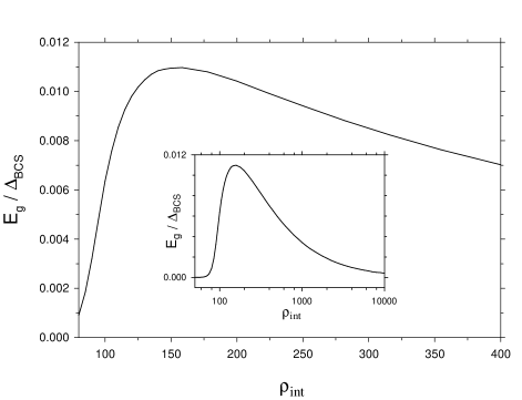
FIG. 5.: Minigap in the single-particle density of states $E_{g}$ versus $\rho_{\rm int}$. The minigap is normalized by the BCS gap value $\Delta_{BCS}$. $E_{g}$ is a nonmonotonic function of $\rho_{\rm int}$, reaching its maximum at $\rho_{\rm int}=160$. The inset shows $E_{g}(\rho_{\rm int})$ on a wider (logarithmic) scale over $\rho_{\rm int}$.

The results (60), (IV) are valid not only below the minigap but also right above it (in which case the real parts of $\theta_{S}$ and $\theta_{N}$ differ from $\pi/2$), providing a comparison between the DOS in the S and N layers. Equation (60) demonstrates the equality of the DOS in the two layers at relatively small $\rho_{\rm int}$ (see Fig. 4, the case $\rho_{\rm int}=80$). Proceeding to the limit of an opaque interface, we should note that the approximation which lead to Eqs. (IV) fails in a narrow vicinity of $E_{g}$ [this fact does not affect the result for the minigap (65) itself, but the incorrect divergence of the DOS at $E=E_{g}$ disappears]. Equations (IV) demonstrate that outside this region, at energies right above the minigap, the DOS in the N layer exceeds the DOS in the S layer by the large factor $\tau_{S}\Delta$ (see Fig. 4, the case $\rho_{\rm int}=2000$).

Finally, we note that the results of the present Section are similar to those obtained by McMillan [8, 9] (see also Ref. [[11]]).

V Anderson limit

In the limit of relatively low interface resistance (the Anderson limit), the theory describing the bilayer can be developed analytically. The condition defining this limit is $\tau_{S}\Delta$, $\tau_{N}\Delta\ll 1$.

First of all, we need to determine $\theta(E)$ [or $Z(E)$] solving Eq. (40) [or Eq. (45)] over the entire range of energies $E$.

In the region $E>\Delta$, the solution of Eq. (45) can be written as $Z=1+\delta Z$, with $|\delta Z|\ll 1$. Keeping terms up to the second order in $\delta Z$, we obtain

$$\delta Z=-\frac{\Delta\left(1-i\tau_{N}E\right)}{E\left(\frac{\tau_{S}+\tau_{N}}{\tau_{S}}-i\tau_{N}E\right)}.$$ (66)

This result is general in the sense that it is valid for arbitrary values of $\rho_{\rm int}$.

At $E<\Delta$, the same calculation as for the minigap leads to the result

$$\sin\theta_{S}=\sin\theta_{N}=\frac{iE_{g}}{\sqrt{E^{2}-E_{g}^{2}}},$$ (67)

with the minigap $E_{g}$ given by Eq. (61). [To avoid confusion, we note that under the less strict limitations for $\tau_{S}\Delta$, $\tau_{N}\Delta$ used in Eq. (61), the BCS-like results (60) and (67) are valid only up to energies of the order of $E_{g}$.]

Now $\mathop{\rm Im}\nolimits\,[\sin\theta_{S}]$ is readily calculated, and in the case of zero temperature, $T=0$, the self-consistency equation (15) can be solved, yielding

$$\frac{\Delta}{\Delta_{BCS}}=\left(\frac{\tau_{S}+\tau_{N}}{\tau_{S}}\right)\left[\frac{\Delta_{BCS}}{2\omega_{D}}\sqrt{1+\left(\frac{\tau_{S}\tau_{N}\omega_{D}}{\tau_{S}+\tau_{N}}\right)^{2}}\right]^{\tau_{N}/\tau_{S}}.$$ (68)

The relation between the order parameter $\Delta$ and the minigap $E_{g}$ is given by Eq. (61), which immediately yields

$$\frac{E_{g}}{\Delta_{BCS}}=\left[\frac{\Delta_{BCS}}{2\omega_{D}}\sqrt{1+\left(\frac{\tau_{S}\tau_{N}\omega_{D}}{\tau_{S}+\tau_{N}}\right)^{2}}\right]^{\tau_{N}/\tau_{S}}.$$ (69)

In the limit of a perfect interface (the Cooper limit), which is defined by the condition $\tau_{S}\tau_{N}\omega_{D}/(\tau_{S}+\tau_{N})\ll 1$, Eq. (69) reproduces classical Cooper’s result [14] generalized to the case of different Fermi parameters in the S and N layers: [15]

$$E_{g}(\rho_{\rm int}\to 0)=2\omega_{D}\exp\left(-\frac{2}{\left<\nu_{0}\lambda\right>}\right),$$ (70)

with the effective interaction parameter

$$\left<\nu_{0}\lambda\right>=\frac{\tau_{S}}{\tau_{S}+\tau_{N}}\,\nu_{0S}\lambda.$$ (71)

This parameter can be considered as a result of averaging with the weighting factors $\tau$, which are proportional to the global normal-metal DOS per unit interval of energy, $\tau\propto{\cal A}d\nu_{0}$ (note that the interaction parameter is zero in the N layer).

At the same time, we would like to emphasize that the Anderson limit does not reduce to the Cooper limit with small corrections. On the contrary, due to the relation $\Delta\ll\omega_{D}$, the Cooper limit’s condition is not satisfied over the most part of the Anderson limit’s validity range; therefore, the minigap $E_{g}$ and the quantities calculated below differ drastically from the Cooper limit expressions.

Now we proceed to calculate the density of the superconducting electrons in the S layer $n_{S}$. On this way, we immediately encounter the problem that the above solution (67) of Eq. (40) at $E<\Delta$ is not accurate enough for our purpose. In fact, as we will see below, the principal contribution to the integral (17) determining $n_{S}$ comes from a narrow region of energies near $E_{g}$. At the same time, Eq. (67) yields $\mathop{\rm Im}\nolimits\,[\sin^{2}\theta_{S}]=0$ and hence no contribution at all from $E<\Delta$. We thus have to calculate a correction to Eq. (67). Assuming this correction to be small, we linearize Eq. (40) and obtain

$$\sin\theta_{S}=\frac{iE_{g}}{\sqrt{E^{2}-E_{g}^{2}}}+X(E),$$ (72)

with

$$X(E)=\frac{\tau_{N}E_{g}}{\left(1+\frac{\tau_{S}}{\tau_{N}}\right)\left[1-\left(\frac{E_{g}}{E}\right)^{2}\right]^{2}},$$ (73)

which is valid for all $E<\Delta$ except for a narrow vicinity of $E_{g}$.

The accurate consideration of the minigap’s vicinity is possible due to the fact that $|Z|\ll 1$ in this region. We define a new dimensionless quantity $\epsilon$ as

$$\frac{E}{E_{g}}=1+\frac{\left(\tau_{S}\Delta\right)^{2/3}}{2\left(1+\frac{\tau_{S}}{\tau_{N}}\right)^{4/3}}\,\epsilon,$$ (74)

and consider the region $|E-E_{g}|\ll E_{g}$. The function $\mathop{\rm Im}\nolimits\,[\sin^{2}\theta_{S}]$, which determines $n_{S}$, has a peak at $\epsilon\sim 1$. An analysis of the coefficients (52) shows that only the terms that contain zeroth, first, and third order in $Z$ should be retained in Eq. (45). Then, after rescaling

$$Z=\frac{\left(\tau_{S}\Delta\right)^{1/3}}{\left(1+\frac{\tau_{S}}{\tau_{N}}\right)^{2/3}}\,Y,$$ (75)

we obtain a cubic equation for the function $Y(\epsilon)$:

$$4Y^{3}-\epsilon Y+i=0,$$ (76)

which can be solved analytically.

The density of the superconducting electrons $n_{S}$ at zero temperature is now readily calculated:

$$\frac{n_{S}}{n_{S}^{BCS}} = \frac{E_{g}}{\Delta_{BCS}}\left\{1+\frac{11\left(\tau_{S}\Delta\right)^{5/6}}{2\pi\left(1+\frac{\tau_{S}}{\tau_{N}}\right)^{4/3}}\right.$$ (78)

$$\left.+\frac{2\tau_{S}\Delta}{\pi\left(1+\frac{\tau_{S}}{\tau_{N}}\right)^{2}}\left[\frac{\tau_{N}}{\tau_{S}}+2\ln\frac{1+\frac{\tau_{S}}{\tau_{N}}}{\tau_{S}\Delta}\right]\right\},$$

with $E_{g}$ given by Eq. (69). The first term in the curly brackets is the principal one; the two other terms become comparable to unity only near the upper limit of applicability of Eq. (78).

The critical temperature of the bilayer $T_{c}$ is determined by Eq. (55). In the Anderson limit, $(\tau_{S}+\tau_{N})/\tau_{S}\tau_{N}\gg T_{c}$, and, with the use of the asymptotic form of the digamma function $\psi(x)\sim\ln x$ at $x\gg 1$, we obtain

$$\frac{T_{c}}{T_{c}^{BCS}}=\frac{E_{g}}{\Delta_{BCS}},$$ (79)

with $E_{g}$ given by Eq. (69). Interestingly, this result explains a discrepancy in the formulas for $T_{c}$ of a thin bilayer that were found by Cooper [14] and McMillan. [8] This discrepancy is discussed in the classical paper by McMillan. [8, 9] We conclude that both cited results are correct, but their applicability ranges are different, although within the Anderson limit. Cooper’s result corresponds to a perfect interface, $\tau_{S}\tau_{N}\omega_{D}/(\tau_{S}+\tau_{N})\ll 1$, whereas McMillan’s formula applies in the case $\tau_{S}\tau_{N}\omega_{D}/(\tau_{S}+\tau_{N})\gg 1$.

Now we can discuss the general structure of the theory describing the bilayer in the Anderson limit. In the limit $\rho_{\rm int}\to 0$, our results for the pairing angle $\theta$ (which is constant over the entire bilayer, $\theta\equiv\theta_{S}=\theta_{N}$) yield expressions which can be obtained from the BCS ones [Eqs. (II C), (22)] if we substitute the BCS order parameter $\Delta_{BCS}$ by the bilayer’s minigap $E_{g}$. At $\rho_{\rm int}>0$, corrections to this simple result are small while the Anderson limit’s conditions are satisfied. Therefore, we obtain a BCS-type theory with $E_{g}$ substituting $\Delta_{BCS}$ in all formulas.

The results of this Section immediately explain the numerical results in the limit of relatively small $\rho_{\rm int}$, shown in Fig. 2. As we have found, the Anderson limit implies the following relations between the quantities under discussion:

$$E_{g} = \frac{\pi}{\gamma}T_{c},$$ (80)

$$n_{S} = \pi\frac{m\sigma_{S}}{e^{2}}E_{g},$$ (81)

which substitute Eqs. (28) and (27). For the Ta/Au bilayer to which the numerical results refer, the Anderson limit is valid at $\rho_{\rm int}<80$ (we see that the values of $\rho_{\rm int}$ can be large although they are relatively small). Therefore, approaching $\rho_{\rm int}=80$, the curves $n_{S}/n_{S}^{BCS}$ and $T_{c}/T_{c}^{BCS}$ tend to coincide, and $\Delta/\Delta_{BCS}$ exceeds them by the large factor $(1+\tau_{N}/\tau_{S})\approx 15$.

The temperature dependence of $\Delta$ and $n_{S}$, shown in Fig. 3, is quite different at $\rho_{\rm int}=90$ and $\rho_{\rm int}=110$; at $\rho_{\rm int}=90$, the curves are much closer to the BCS behavior. This is also explained by approaching the Anderson limit, where the curves coincide with the BCS ones.

The DOS in the S and N layers coincide in the Anderson limit [Eqs. (60), (67)], showing the standard BCS-like peculiarity at $E=E_{g}$. The tendency to such behavior is illustrated by the DOS curve for $\rho_{\rm int}=80$ in Fig. 4.

VI Parallel critical field

We proceed to calculate the critical magnetic field $H_{c}$ directed along the plane of the bilayer. As it was mentioned in Sec. II B, in the presence of an external magnetic field, the superconducting phase gradient in the Usadel equations (II B) must be substituted by its gauge invariant form, which can be expressed via the supercurrent velocity ${\bf v}$. The spatial distribution of ${\bf v}$ in the bilayer can be found as follows.

Let us direct the $x$-axis along the magnetic field ${\bf H}$. The supercurrents ${\bf j}=-en{\bf v}$ are directed along the bilayer and perpendicularly to ${\bf H}$, i.e., ${\bf j}=(0,j(z),0)$ and ${\bf v}=(0,v(z),0)$. Near $H_{c}$, the magnetic field inside the bilayer is uniform, so the vector potential can be chosen as ${\bf A}=(0,-zH,0)$. The supercurrent velocity distribution is determined by the equation $\nabla\times{\bf v}=e{\bf H}/m$. Another essential point is the continuity of ${\bf v}$ at the SN interface, which follows from the continuity of the superconducting phase $\varphi$ [see the boundary condition (14)]. The result is

$$v(z)=v_{0}-\frac{eH}{m}z,$$ (82)

where $v_{0}$ is the supercurrent velocity at the interface, which must be determined from the condition that the total charge transfer across the bilayer’s cross-section is zero:

$$\int_{-d_{N}}^{d_{S}}j(z)\,dz=0,$$ (83)

leading to

$$v_{0}=\left(\frac{eH}{2m}\right)\frac{n_{S}d_{S}^{2}-n_{N}d_{N}^{2}}{n_{S}d_{S}+n_{N}d_{N}}.$$ (84)

The density of the superconducting electrons is constant in each layer ($n_{S}$ and $n_{N}$).

Near $H_{c}$, the superconducting correlations are small, $|\theta|\ll 1$, and the Usadel equation (8) for the paring angle $\theta(z,E)$ can be linearized:

$$\frac{D_{N}}{2}\frac{\partial^{2}\theta_{N}}{\partial z^{2}}+\left(iE-2m^{2}D_{N}\,{\bf v}^{2}\right)\theta_{N} = 0,$$ (86)

$$\frac{D_{S}}{2}\frac{\partial^{2}\theta_{S}}{\partial z^{2}}+\left(iE-2m^{2}D_{S}\,{\bf v}^{2}\right)\theta_{S}+\left|\Delta\right| = 0.$$ (87)

At the same time, the second Usadel equation (9) is trivial: its l.h.s. is proportional to

$$\nabla\left(\sin^{2}\theta\,\,{\bf v}\right)=\sin 2\theta\,\,\nabla\theta\,\,{\bf v}+\sin^{2}\theta\,\,\nabla{\bf v},$$ (88)

where both terms vanish due to the fact that $\nabla\theta$ is directed along the $z$-axis whereas ${\bf v}$ is parallel to the $y$-axis.

The pairing angle $\theta$ is almost spatially constant in each layer; this allows us to average each of Eqs. (VI) over the thickness of the corresponding layer, obtaining

$$\left.\frac{\partial\theta_{N}}{\partial z}\right|_{z=0} = \frac{2d_{N}}{D_{N}}\left(E_{N}-iE\right)\theta_{N},$$ (90)

$$\left.\frac{\partial\theta_{S}}{\partial z}\right|_{z=0} = \frac{2d_{S}}{D_{S}}\left[\left(iE-E_{S}\right)\theta_{S}+\left|\Delta\right|\right],$$ (91)

where

$$E_{N} = 2m^{2}D_{N}\left<{\bf v}^{2}(z)\right>_{N},$$ (92)

$$E_{S} = 2m^{2}D_{S}\left<{\bf v}^{2}(z)\right>_{S}$$ (93)

are $H$-dependent energies. Using Eqs. (82), (84), we express them via $H_{c}$ and the densities of the superconducting electrons:

$$E_{S}=\frac{D_{S}\,e^{2}H_{c}^{2}}{6}\left[d_{S}^{2}+3d_{N}^{2}\frac{n_{N}^{2}\left(d_{S}+d_{N}\right)^{2}}{\left(n_{S}d_{S}+n_{N}d_{N}\right)^{2}}\right],$$ (94)

and $E_{N}$ is obtained by the interchange of all the S and N indices.

Substituting (VI) into the boundary conditions (32) (which should be linearized), we find

$$\theta_{N} = \tau_{S}\left|\Delta\right|\left/\left\{\tau_{S}E_{S}+\tau_{N}E_{N}+\tau_{S}\tau_{N}E_{S}E_{N}-\tau_{S}\tau_{N}E^{2}\right.\right.$$ (97)

$$\phantom{\tau_{S}\left|\Delta\right|/\bigl{\{}}\left.-iE\left[\tau_{S}+\tau_{N}+\tau_{S}\tau_{N}\left(E_{S}+E_{N}\right)\right]\right\},$$

$$\theta_{S} = \left(1+\tau_{N}E_{N}-i\tau_{N}E\right)\theta_{N}.$$ (98)

The order parameter $\Delta$ cancels out from the self-consistency equation (15). However, the resulting equation alone does not suffice for determining $H_{c}(T)$ because it contains $E_{S}$ and $E_{N}$, which are functions of $n_{N}/n_{S}$. Therefore, to obtain a closed system, we must consider the self-consistency equation together with the equation determining the ratio $n_{N}/n_{S}$; the latter equation is obtained from Eq. (17). The resulting system of two nonlinear equations for the quantities $H_{c}$ and $n_{N}/n_{S}$ is

$$\ln\frac{2\omega_{D}}{\Delta_{BCS}} = \int_{0}^{\omega_{D}}dE\,\tanh\!\left(\!\frac{E}{2T}\!\right)\frac{\mathop{\rm Im}\nolimits\theta_{S}}{\left|\Delta\right|},$$ (100)

$$\frac{n_{N}}{n_{S}} = \frac{\sigma_{N}\int_{0}^{\infty}dE\,\tanh\!\left(\frac{E}{2T}\right)\mathop{\rm Im}\nolimits\theta_{N}^{2}}{\sigma_{S}\int_{0}^{\infty}dE\,\tanh\!\left(\frac{E}{2T}\right)\mathop{\rm Im}\nolimits\theta_{S}^{2}},$$ (101)

with $\theta_{N}$ and $\theta_{S}$ given by Eqs. (VI). The first equation of the system, Eq. (100), can be written via the digamma functions, thus taking exactly the same form as Eq. (135) below (which determines the perpendicular upper critical field) if we denote ${\cal E}_{S}=E_{S}+1/\tau_{S}$, ${\cal E}_{N}=E_{N}+1/\tau_{N}$.

In the limit $\rho_{\rm int}\to\infty$, Eqs. (VI) lead to the BCS result. In this case, the layers uncouple, the density of the superconducting electrons in the N layer vanishes, $n_{N}/n_{S}\to 0$, and Eq. (100) finally yields

$$\ln\frac{T_{c}^{BCS}}{T}=\psi\left(\frac{1}{2}+\frac{D_{S}\left[eH_{c}^{BCS}d_{S}\right]^{2}}{12\pi T}\right)-\psi\left(\frac{1}{2}\right),$$ (102)

which determines the parallel critical field $H_{c}^{BCS}(T)$ of a thin superconducting film. Another immediate consequence of Eqs. (VI) is the critical temperature of the bilayer $T_{c}$, which can be found from the condition $H_{c}(T_{c})=0$: in this case, Eqs. (VI) reproduce Eq. (55).

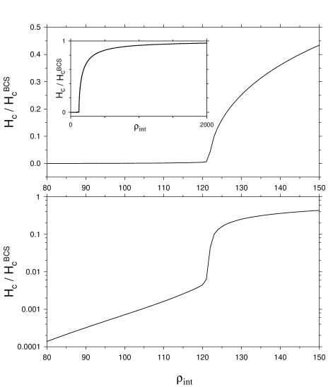
FIG. 6.: Parallel critical field $H_{c}$, normalized by the BCS value, versus $\rho_{\rm int}$ at zero temperature. The upper and lower graphs differ only in the scaling of the ordinate axis (normal and logarithmic, respectively). The nature of the steep behavior of $H_{c}$ at $\rho_{\rm int}=120$–$123$, which is best seen from the lower graph, is explained in the text. The inset shows $H_{c}(\rho_{\rm int})$ on a wider scale over $\rho_{\rm int}$.

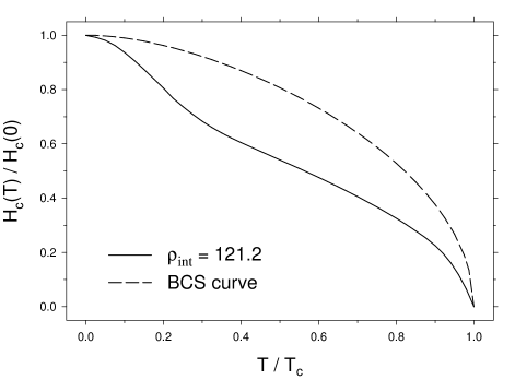
FIG. 7.: Temperature dependence of the parallel critical field $H_{c}$ at $\rho_{\rm int}=121.2$. The experimental value of $H_{c}(0)$, analyzed with the use of the results shown in Fig. 6, suggests that this value of $\rho_{\rm int}$ corresponds to the experiment by Kasumov et al. [2] The critical field is normalized by its zero-temperature value, and the temperature is normalized by the corresponding $T_{c}$. For comparison, the same dependence is plotted for the BCS case.

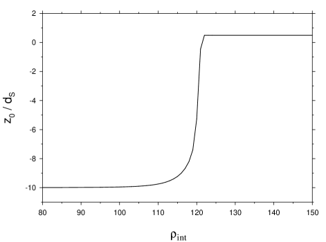
FIG. 8.: Position of the stationary point $z_{0}$ of the supercurrent distribution versus $\rho_{\rm int}$ at zero temperature. The coordinate $z_{0}$ is normalized by the S layer thickness $d_{S}$. The fast shift in $z_{0}$ from the center of the S layer at large $\rho_{\rm int}$ to (nearly) the center of the N layer at small $\rho_{\rm int}$ corresponds to the steep drop in $H_{c}$, shown in Fig. 6.

The system of equations (VI) can be solved numerically at arbitrary values of the temperature $T$ and the interface resistance $\rho_{\rm int}$; the results for $H_{c}$ are presented in Figs. 6, 7.

A remarkable feature of the function $H_{c}(\rho_{\rm int})$ at zero temperature (Fig. 6) is the steep behavior of $H_{c}$ at $\rho_{\rm int}=120$–$123$. This feature is due to rearrangement of the supercurrents inside the bilayer, which occurs in the following way. The supercurrent velocity changes across the thickness of the bilayer according to the simple linear law (82). This supercurrent distribution may be characterized by the position of the stationary point $z_{0}$, where the supercurrent velocity is zero: $v(z_{0})=0$, hence $z_{0}=mv_{0}/eH$. At large values of the interface resistance $\rho_{\rm int}$, the density of the superconducting electrons in the N layer is very small, $n_{N}/n_{S}\ll 1$, and the supercurrents circulate only in the S part of the system; this case corresponds to

$$z_{0}=\frac{d_{S}}{2}.$$ (103)

Then, while decreasing $\rho_{\rm int}$, a shift in $z_{0}$ occurs. Now the supercurrents in the S layer are not compensated (in the sense of the charge transfer); therefore, they must be compensated by the supercurrents in the N layer, which are enhanced due to significant increase in $n_{N}$. This situation corresponds to the beginning of the drop in $H_{c}$. The ratio of the superconducting electrons’ densities grows rapidly, approaching the Anderson limit value $n_{N}/n_{S}=\sigma_{N}/\sigma_{S}$ (see Sec. VI A below); simultaneously, $z_{0}$ tends to

$$z_{0}=\frac{\sigma_{S}d_{S}^{2}-\sigma_{N}d_{N}^{2}}{2\left(\sigma_{S}d_{S}+\sigma_{N}d_{N}\right)},$$ (104)

and the steep drop in $H_{c}$ finishes. For the bilayer to which the numerical results refer, $d_{S}\ll d_{N}$ and $\sigma_{S}\ll\sigma_{N}$, so Eq. (104) yields $z_{0}\approx-d_{N}/2$.

This scenario is illustrated by Fig. 8, which has been obtained numerically.

The analytical solution of Eqs. (VI) at zero temperature in the Anderson limit is presented below.

A $H_{c}$ at zero temperature in the Anderson limit

In the zero-temperature Anderson limit (defined by the conditions $\tau_{S}E_{S}$, $\tau_{N}E_{N}\ll 1$), the ratio of the superconducting electrons’ densities (101) becomes independent of the magnetic field, $n_{N}/n_{S}=\sigma_{N}/\sigma_{S}$, and the self-consistency equation (100) yields

$$\frac{\tau_{S}E_{S}+\tau_{N}E_{N}}{\tau_{S}+\tau_{N}}=\frac{\Delta_{BCS}}{2}\left[\frac{\Delta_{BCS}}{2\omega_{D}}\sqrt{1+\left(\frac{\tau_{S}\tau_{N}\omega_{D}}{\tau_{S}+\tau_{N}}\right)^{2}}\right]^{\frac{\tau_{N}}{\tau_{S}}}$$ (105)

which determines $H_{c}$. This result can be compared to the BCS case, which corresponds to the limit $\rho_{\rm int}\to\infty$. In this case, the density of the superconducting electrons in the N layer vanishes, $n_{N}/n_{S}\to 0$, and the self-consistency equation yields

$$E_{S}^{BCS}=\frac{\Delta_{BCS}}{2},$$ (106)

where $E_{S}^{BCS}$ is given by Eq. (94) with $n_{N}=0$. Finally,

$$H_{c}^{BCS}=\frac{\sqrt{3}\Phi_{0}}{\pi\,\xi_{BCS}\,d_{S}},\qquad\xi_{BCS}=\sqrt{\frac{D_{S}}{\Delta_{BCS}}},$$ (107)

where $\Phi_{0}=\pi/e$ is the flux quantum, and $\xi_{BCS}$ is the correlation length in the dirty limit.

Remarking that the r.h.s. of Eq. (105) is identical to $E_{g}/2$ with the minigap $E_{g}$ given by Eq. (69), we see that equation (105), determining the parallel critical field of the bilayer in the Anderson limit, is obtained from the BCS equation (106) if we substitute the order parameter $\Delta_{BCS}$ by the minigap $E_{g}$ (in accordance with the results of Sec. V) and the $H$-dependent energy $E_{S}^{BCS}$ by the corresponding averaged quantity $(\tau_{S}E_{S}+\tau_{N}E_{N})/(\tau_{S}+\tau_{N})$.

The explicit result for the parallel critical field of the bilayer, obtained from Eq. (105), can be cast into a BCS-like form:

$$H_{c}=\frac{\sqrt{3}\Phi_{0}}{\pi\xi d_{\rm eff}}.$$ (108)

The bilayer’s correlation length $\xi$ is the characteristic space scale on which the order parameter (or the pairing angle $\theta$, or the Green function) varies in the absence of the magnetic field. In the Anderson limit (under discussion), the explicit formula for $\xi$ is a natural generalization of the BCS expression [see Eq. (107)] which implies that $D_{S}$ must be substituted by the averaged diffusion constant $\left<D\right>$ and $\Delta_{BCS}$ must be substituted (in accordance with the results of Sec. V) by the bilayer’s characteristic energy scale, the minigap $E_{g}$ [Eq. (69)]:

$$\xi=\sqrt{\frac{\left<D\right>}{E_{g}}},\qquad\left<D\right>=\frac{\tau_{S}D_{S}+\tau_{N}D_{N}}{\tau_{S}+\tau_{N}}.$$ (109)

The effective thickness of the bilayer in Eq. (108) is

$$d_{\rm eff}=\Bigl{[}\left(\sigma_{S}d_{S}+\sigma_{N}d_{N}\right)\left(\sigma_{S}d_{S}^{3}+\sigma_{N}d_{N}^{3}\right)$$ (110)

$$\left.+3\sigma_{S}\sigma_{N}d_{S}d_{N}\left(d_{S}+d_{N}\right)^{2}\Bigr{]}^{1/2}\right/\left(\sigma_{S}d_{S}+\sigma_{N}d_{N}\right).$$ (111)

In the case of equal conductivities, $\sigma_{S}=\sigma_{N}$, the effective thickness is simply the geometrical one: $d_{\rm eff}=d_{S}+d_{N}$. This case corresponds to a uniform density of the superconducting electrons, $n_{S}=n_{N}$, which implies a continuous distribution of the supercurrents, centered at the middle of the bilayer [this can be also seen from Eq. (104) which yields $z_{0}=(d_{S}+d_{N})/2$ in the case $\sigma_{S}=\sigma_{N}$]. However, in a more subtle situation when the conductivities are different, the density of the supercurrent experiences a jump at the SN interface; this nontrivial supercurrent distribution results in the nonequivalence of $d_{\rm eff}$ to the geometrical thickness of the bilayer.

VII Perpendicular upper critical field

Now we turn to calculating the upper critical field $H_{c2}$ perpendicular to the plane of the bilayer.

As in the case of the parallel critical field, we start with discussing the supercurrent distribution, which is now a function of the sample boundaries in the $xy$-plane, perpendicular to the magnetic field ${\bf H}$ (the magnetic field is directed along the $z$-axis). The infinite bilayer under consideration can be thought of as a disk of a large radius; let us assume $x=0$, $y=0$ at the axis of the disk. Then the supercurrent distribution is axially symmetric, and, with the gauge chosen as ${\bf A}=\left[{\bf Hr}\right]/2$, the superconducting phase must be constant, $\varphi=0$, which yields a simple result for the supercurrent velocity: ${\bf v}=e{\bf A}/m$.

Near $H_{c2}$, the superconducting correlations are small, $|\theta|\ll 1$, and the Usadel equations can be linearized:

$$-\frac{D}{2}\left(-i\nabla+2e{\bf A}\right)^{2}\theta+iE\theta+\Delta = 0,$$ (113)

$${\bf A}\nabla\theta = 0.$$ (114)

The second of these equations is trivially satisfied because $\theta({\bf r})$ is axially symmetric.

Thus, the Usadel equations reduce to the single Eq. (113) for the pairing angle $\theta({\bf r},E)$. Introducing the cylindrical coordinates ${\bf r}\leftrightarrow(z,\mathchoice{{\hbox{\boldmath$\displaystyle\rho$}}}{{\hbox{\boldmath$\textstyle\rho$}}}{{\hbox{\boldmath$\scriptstyle\rho$}}}{{\hbox{\boldmath$\scriptscriptstyle\rho$}}})$ and denoting $\hat{\bf P}=-i\nabla_{\mathchoice{{\hbox{\boldmath$\displaystyle\rho$}}}{{\hbox{\boldmath$\textstyle\rho$}}}{{\hbox{\boldmath$\scriptstyle\rho$}}}{{\hbox{\boldmath$\scriptscriptstyle\rho$}}}}+2e{\bf A}(\mathchoice{{\hbox{\boldmath$\displaystyle\rho$}}}{{\hbox{\boldmath$\textstyle\rho$}}}{{\hbox{\boldmath$\scriptstyle\rho$}}}{{\hbox{\boldmath$\scriptscriptstyle\rho$}}})$, we rewrite this equation as

$$\frac{D_{N}}{2}\frac{\partial^{2}\theta_{N}}{\partial z^{2}}-\frac{D_{N}}{2}\hat{\bf P}^{2}\theta_{N}+iE\theta_{N} = 0,$$ (116)

$$\frac{D_{S}}{2}\frac{\partial^{2}\theta_{S}}{\partial z^{2}}-\frac{D_{S}}{2}\hat{\bf P}^{2}\theta_{S}+iE\theta_{S}+\Delta = 0.$$ (117)

We cannot solve these equations straightforwardly because near the upper critical field, the order parameter $\Delta({\mathchoice{{\hbox{\boldmath$\displaystyle\rho$}}}{{\hbox{\boldmath$\textstyle\rho$}}}{{\hbox{\boldmath$\scriptstyle\rho$}}}{{\hbox{\boldmath$\scriptscriptstyle\rho$}}}})$ is a nontrivial unknown function of the in-plane coordinate $\textstyle\rho$ (while the $z$-dependence is absent due to the small thickness of the bilayer). In this situation, we employ the following approach.

Averaging each of Eqs. (VII) over the thickness of the corresponding layer, we obtain

$$\left.\frac{\partial\theta_{N}}{\partial z}\right|_{z=0} = \frac{2d_{N}}{D_{N}}\left(\frac{D_{N}}{2}\hat{\bf P}^{2}\theta_{N}-iE\theta_{N}\right),$$ (119)

$$\left.\frac{\partial\theta_{S}}{\partial z}\right|_{z=0} = \frac{2d_{S}}{D_{S}}\left(-\frac{D_{S}}{2}\hat{\bf P}^{2}\theta_{S}+iE\theta_{S}+\Delta\right).$$ (120)

The averaged pairing angles entering the r.h.s. of Eqs. (VII) are

$$\theta_{N}(\mathchoice{{\hbox{\boldmath$\displaystyle\rho$}}}{{\hbox{\boldmath$\textstyle\rho$}}}{{\hbox{\boldmath$\scriptstyle\rho$}}}{{\hbox{\boldmath$\scriptscriptstyle\rho$}}},E) = \frac{1}{d_{N}}\int_{-d_{N}}^{0}dz\,\theta_{N}(z,\mathchoice{{\hbox{\boldmath$\displaystyle\rho$}}}{{\hbox{\boldmath$\textstyle\rho$}}}{{\hbox{\boldmath$\scriptstyle\rho$}}}{{\hbox{\boldmath$\scriptscriptstyle\rho$}}},E),$$ (122)

$$\theta_{S}(\mathchoice{{\hbox{\boldmath$\displaystyle\rho$}}}{{\hbox{\boldmath$\textstyle\rho$}}}{{\hbox{\boldmath$\scriptstyle\rho$}}}{{\hbox{\boldmath$\scriptscriptstyle\rho$}}},E) = \frac{1}{d_{S}}\int_{0}^{d_{S}}dz\,\theta_{S}(z,\mathchoice{{\hbox{\boldmath$\displaystyle\rho$}}}{{\hbox{\boldmath$\textstyle\rho$}}}{{\hbox{\boldmath$\scriptstyle\rho$}}}{{\hbox{\boldmath$\scriptscriptstyle\rho$}}},E).$$ (123)

Substituting Eqs. (VII) into the boundary conditions (32) (which should be linearized), we obtain a system of two differential equations for the function $\theta(\mathchoice{{\hbox{\boldmath$\displaystyle\rho$}}}{{\hbox{\boldmath$\textstyle\rho$}}}{{\hbox{\boldmath$\scriptstyle\rho$}}}{{\hbox{\boldmath$\scriptscriptstyle\rho$}}},E)$:

$$\tau_{N}\left(\frac{D_{N}}{2}\hat{\bf P}^{2}\theta_{N}-iE\theta_{N}\right)\! = \tau_{S}\left(-\frac{D_{S}}{2}\hat{\bf P}^{2}\theta_{S}+iE\theta_{S}+\Delta\right)$$ (124)

$$= \theta_{S}-\theta_{N}.$$ (125)

From the vicinity of the superconductive transition it follows that the pairing angle $\theta$ depends on the order parameter $\Delta$ linearly:

$$\theta_{N}(\mathchoice{{\hbox{\boldmath$\displaystyle\rho$}}}{{\hbox{\boldmath$\textstyle\rho$}}}{{\hbox{\boldmath$\scriptstyle\rho$}}}{{\hbox{\boldmath$\scriptscriptstyle\rho$}}},E) = \frac{\Delta\left(\mathchoice{{\hbox{\boldmath$\displaystyle\rho$}}}{{\hbox{\boldmath$\textstyle\rho$}}}{{\hbox{\boldmath$\scriptstyle\rho$}}}{{\hbox{\boldmath$\scriptscriptstyle\rho$}}}\right)}{\alpha_{N}\left(E\right)},$$ (127)

$$\theta_{S}(\mathchoice{{\hbox{\boldmath$\displaystyle\rho$}}}{{\hbox{\boldmath$\textstyle\rho$}}}{{\hbox{\boldmath$\scriptstyle\rho$}}}{{\hbox{\boldmath$\scriptscriptstyle\rho$}}},E) = \frac{\Delta\left(\mathchoice{{\hbox{\boldmath$\displaystyle\rho$}}}{{\hbox{\boldmath$\textstyle\rho$}}}{{\hbox{\boldmath$\scriptstyle\rho$}}}{{\hbox{\boldmath$\scriptscriptstyle\rho$}}}\right)}{\alpha_{S}\left(E\right)},$$ (128)

where the functions $\alpha_{N}(E)$ and $\alpha_{S}(E)$ are spatially independent. Then Eqs. (125) can be rewritten as

$$\frac{D_{N}}{2}\hat{\bf P}^{2}\Delta(\mathchoice{{\hbox{\boldmath$\displaystyle\rho$}}}{{\hbox{\boldmath$\textstyle\rho$}}}{{\hbox{\boldmath$\scriptstyle\rho$}}}{{\hbox{\boldmath$\scriptscriptstyle\rho$}}})=\left[iE+\frac{1}{\tau_{N}}\left(\frac{\alpha_{N}\left(E\right)}{\alpha_{S}\left(E\right)}-1\right)\right]\Delta(\mathchoice{{\hbox{\boldmath$\displaystyle\rho$}}}{{\hbox{\boldmath$\textstyle\rho$}}}{{\hbox{\boldmath$\scriptstyle\rho$}}}{{\hbox{\boldmath$\scriptscriptstyle\rho$}}}),$$ (130)

$$\frac{D_{S}}{2}\hat{\bf P}^{2}\Delta(\mathchoice{{\hbox{\boldmath$\displaystyle\rho$}}}{{\hbox{\boldmath$\textstyle\rho$}}}{{\hbox{\boldmath$\scriptstyle\rho$}}}{{\hbox{\boldmath$\scriptscriptstyle\rho$}}})=\left[iE+\frac{1}{\tau_{S}}\left(\frac{\alpha_{S}\left(E\right)}{\alpha_{N}\left(E\right)}-1\right)+\alpha_{S}(E)\right]\Delta(\mathchoice{{\hbox{\boldmath$\displaystyle\rho$}}}{{\hbox{\boldmath$\textstyle\rho$}}}{{\hbox{\boldmath$\scriptstyle\rho$}}}{{\hbox{\boldmath$\scriptscriptstyle\rho$}}}).$$ (131)

We see that the order parameter must be an eigenfunction of the differential operator $\hat{\bf P}^{2}$. Moreover, in order to obtain the largest value of $H_{c2}$, we should choose the eigenfunction corresponding to the lowest eigenvalue (in complete analogy with Refs. [[16, 17]]). The solution of the emerging eigenvalue problem is readily found thanks to its formal equivalence to the problem of determining the Landau levels of a two-dimensional particle with the “mass” $1/D$ and the charge $-2e$ in the uniform magnetic field ${\bf H}$ directed along the third dimension. The lowest Landau level is $DeH$; the function $\alpha_{S}(E)$ is straightforwardly determined,

$$\alpha_{S}(E)=D_{S}\,eH-iE+\frac{\tau_{N}\left(D_{N}\,eH-iE\right)}{\tau_{S}\left[1+\tau_{N}\left(D_{N}\,eH-iE\right)\right]},$$ (132)

and we substitute $\theta_{S}(\mathchoice{{\hbox{\boldmath$\displaystyle\rho$}}}{{\hbox{\boldmath$\textstyle\rho$}}}{{\hbox{\boldmath$\scriptstyle\rho$}}}{{\hbox{\boldmath$\scriptscriptstyle\rho$}}},E)$ into the self-consistency equation (15). The order parameter $\Delta(\mathchoice{{\hbox{\boldmath$\displaystyle\rho$}}}{{\hbox{\boldmath$\textstyle\rho$}}}{{\hbox{\boldmath$\scriptstyle\rho$}}}{{\hbox{\boldmath$\scriptscriptstyle\rho$}}})$ cancels out, and the resulting equation, which determines $H_{c2}(T)$, can be cast into the form

  

$$\ln\frac{T_{c}^{BCS}}{T} = -\frac{\tau_{N}}{\tau_{S}+\tau_{N}}\ln\sqrt{1+\left(\frac{\tau_{S}+\tau_{N}}{\tau_{S}\tau_{N}\omega_{D}}\right)^{2}}-\psi\left(\frac{1}{2}\right)$$ (135)

$$+\frac{1}{2}\left[1+\frac{{\cal E}_{S}-{\cal E}_{N}}{\sqrt{\left({\cal E}_{S}-{\cal E}_{N}\right)^{2}+4/\tau_{S}\tau_{N}}}\right]\psi\left(\frac{1}{2}+\frac{1}{4\pi T}\left[{\cal E}_{S}+{\cal E}_{N}+\sqrt{\left({\cal E}_{S}-{\cal E}_{N}\right)^{2}+\frac{4}{\tau_{S}\tau_{N}}}\right]\right)$$

$$+\frac{1}{2}\left[1-\frac{{\cal E}_{S}-{\cal E}_{N}}{\sqrt{\left({\cal E}_{S}-{\cal E}_{N}\right)^{2}+4/\tau_{S}\tau_{N}}}\right]\psi\left(\frac{1}{2}+\frac{1}{4\pi T}\left[{\cal E}_{S}+{\cal E}_{N}-\sqrt{\left({\cal E}_{S}-{\cal E}_{N}\right)^{2}+\frac{4}{\tau_{S}\tau_{N}}}\right]\right),$$

  

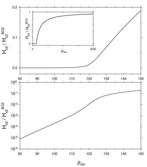
FIG. 9.: Perpendicular upper critical field $H_{c2}$, normalized by its BCS value, versus $\rho_{\rm int}$ at zero temperature. The upper and lower graphs differ only in the scaling of the ordinate axis (normal and logarithmic, respectively). The inset shows $H_{c2}(\rho_{\rm int})$ on a wider scale over $\rho_{\rm int}$.

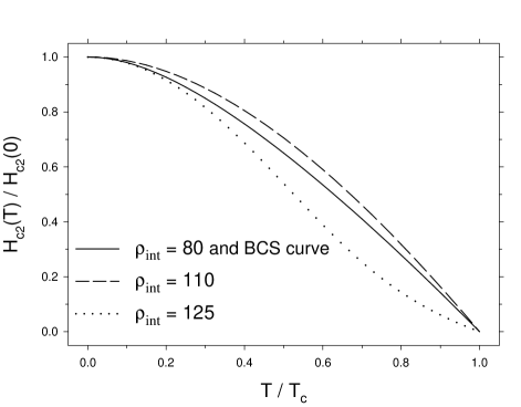
FIG. 10.: Temperature dependence of the perpendicular upper critical field $H_{c2}$ at $\rho_{\rm int}=80$, 110, 125, and in the BCS case. In each case, the critical field is normalized by its zero-temperature value, and the temperature is normalized by the corresponding $T_{c}$. According to the results of Sec. V, the curves in the BCS and Anderson ($\rho_{\rm int}=80$) limits coincide. At intermediate values of $\rho_{\rm int}$, the curves can lie both above ($\rho_{\rm int}=110$) and below ($\rho_{\rm int}=125$) the BCS curve.

where

$${\cal E}_{S} = D_{S}\,eH_{c2}+\frac{1}{\tau_{S}},$$ (136)

$${\cal E}_{N} = D_{N}\,eH_{c2}+\frac{1}{\tau_{N}}$$ (137)

are $H$-dependent energies. The logarithmic term in the r.h.s. of Eq. (135) takes account of the finiteness of the Debye energy $\omega_{D}$; it becomes important only in the limit of a perfect interface (the Cooper limit), i.e., when $\tau_{S}\tau_{N}\omega_{D}/(\tau_{S}+\tau_{N})\ll 1$.

In the limit $\rho_{\rm int}\to\infty$, Eq. (135) yields the classical result of Maki [18] and de Gennes [19] for the BCS case,

$$\ln\frac{T_{c}^{BCS}}{T}=\psi\left(\frac{1}{2}+\frac{D_{S}\,eH_{c2}^{BCS}}{2\pi T}\right)-\psi\left(\frac{1}{2}\right),$$ (138)

which is valid for bulk superconductors and superconductive layers of arbitrary thickness (when the magnetic field is directed perpendicularly to them). Another immediate consequence of Eq. (135) is the critical temperature of the bilayer $T_{c}$, which can be found from the condition $H_{c2}(T_{c})=0$: in this case, Eq. (135) reproduces Eq. (55).

Equation (135) can be solved numerically at arbitrary values of the temperature $T$ and the interface resistance $\rho_{\rm int}$; the results for $H_{c2}$ are presented in Figs. 9, 10.

The analytical solution of Eq. (135) at zero temperature in the Anderson limit is presented below.

A $H_{c2}$ at zero temperature in the Anderson limit

In the zero-temperature Anderson limit (defined by the conditions $D_{S}\,eH_{c2}\ll 1/\tau_{S}$, $D_{N}\,eH_{c2}\ll 1/\tau_{N}$), Eq. (135) yields

$$\frac{H_{c2}}{H_{c2}^{BCS}}=\frac{\left(\tau_{S}+\tau_{N}\right)D_{S}}{\tau_{S}D_{S}+\tau_{N}D_{N}}\left[\frac{\Delta_{BCS}}{2\omega_{D}}\sqrt{1+\left(\frac{\tau_{S}\tau_{N}\omega_{D}}{\tau_{S}+\tau_{N}}\right)^{2}}\right]^{\frac{\tau_{N}}{\tau_{S}}}$$ (139)

where the zero-temperature BCS value of the upper critical field, as follows from Eq. (138), is

$$H_{c2}^{BCS}=\frac{\Delta_{BCS}}{2eD_{S}}=\frac{\Phi_{0}}{2\pi\xi_{BCS}^{2}}.$$ (140)

It is instructive to rewrite the perpendicular upper critical field of the bilayer (139) in the standard BCS-like form

$$H_{c2}=\frac{\Phi_{0}}{2\pi\xi^{2}},$$ (141)

where $\xi$ is the bilayer’s correlation length given by Eq. (109) [the physical interpretation of this result for $\xi$ precedes Eq. (109)].

VIII SNS, NSN, SNINS, NSISN, and superlattices

Our results for $\Delta$, $n_{S}$, $T_{c}$, $E_{g}$, $\nu(E)$, and $H_{c2}$ (i.e., all the results except $H_{c}$) can be directly applied to more complicated structures such as SNS and NSN trilayers, SNINS and NSISN systems, and SN superlattices.

Let us consider, for example, a symmetric SNS trilayer consisting of two identical S layers of thickness $d_{S}$ separated by a N layer of thickness $2d_{N}$. The SN interfaces can have arbitrary (but equal) resistances. As before, the $z$-axis is perpendicular to the plane of the structure. This trilayer can be imagined as composed of two identical bilayers perfectly joined together along the N sides. Indeed, the pairing angle $\theta$ has zero $z$-derivative on the outer surfaces of the bilayers, thus producing the correct (symmetric in the $z$-direction) solution for $\theta$ in the resulting trilayer. Consequently, the symmetric SNS trilayer has exactly the same physical properties [$\Delta$, $n_{S}$, $T_{c}$, $E_{g}$, $\nu(E)$, $H_{c2}$] as the SN bilayer considered in the present paper. The only point where the above reasoning fails is the calculation of the parallel critical field $H_{c}$. In this case, the combination of the supercurrent distributions in the two bilayers does not yield the correct distribution in the resulting SNS trilayer, which implies that the Usadel equations for the two systems are different.

Evidently, the above reasoning, based on the formal equivalence of the outer-surface boundary condition for the bilayer to the symmetry-caused condition in the middle of the SNS trilayer, also holds for symmetric NSN trilayers (N layers of thickness $d_{N}$, S layer of thickness $2d_{S}$, identical SN interfaces) and SN superlattices (N layers of thickness $2d_{N}$, S layers of thickness $2d_{S}$, identical SN interfaces). Moreover, the same applies to systems composed of two bilayers in nonideal contact with each other: SNINS and NSISN (where I stands for an arbitrary potential barrier), because the presence of a potential barrier does not violate the applicability of the symmetry argument. Thus, all the results obtained for the bilayer (except $H_{c}$) are also valid for these structures.

IX Discussion

An essential property of the bilayer used throughout the paper is its small thickness. Now we shall argue that the bilayer studied in the experiment by Kasumov et al. [2] (and to which our numerical results refer) can be considered thin. The Usadel equations (III) imply that the characteristic space scale of the bilayer’s properties variation is $\sqrt{D_{N,S}/E_{0}}$ for the N and S layers, respectively. However, the correct determination of the characteristic energy scale $E_{0}$ is a nontrivial problem. Our results suggest that $E_{0}$ is always smaller than the order parameter $\Delta$: in the BCS limit ($\rho_{\rm int}\to\infty$), $E_{0}$ approaches $\Delta$, whereas in the opposite (Anderson) limit, $E_{0}$ is determined by the minigap $E_{g}$ [see Eq. (61)]. For the following discussion, it is convenient to write the condition of the small thickness of the bilayer as

$$d_{N,S}\ll\sqrt{\frac{\Delta}{E_{0}}}\,\sqrt{\frac{\Delta_{BCS}}{\Delta}}\,\sqrt{\frac{D_{N,S}}{\Delta_{BCS}}}.$$ (142)

The individual layers’ thicknesses are $d_{N}=$ 100 nm and $d_{S}=$ 5 nm. The third multiplier (the BCS correlation length) in the r.h.s. of the condition (142) equals 194 nm and 16 nm for the N and S layers, respectively. At the same time, each of the first two multipliers in the r.h.s. of the condition (142) exceeds unity. We can thus conclude that the bilayer can indeed be considered thin.

Now we turn to a possible experimental application of our results. Our results provide a method for determining $\rho_{\rm int}$, a very important parameter of the bilayer which is not directly measurable. By analyzing the experimental [2, 12] values $T_{c}=0.4$ K and $H_{c}=0.1$ T, we get $\rho_{\rm int}\approx 111$ and $\rho_{\rm int}\approx 121$, respectively. Within the experimental accuracy of the bilayer’s parameters, the two estimates for $\rho_{\rm int}$ should be considered close. Interestingly, the value $\rho_{\rm int}\approx 121$ extracted from the measured value of $H_{c}$ corresponds to the extremely narrow region of the steep drop in $H_{c}(\rho_{\rm int})$ (see Fig. 6).

Finally, we wish to remark on a peculiarity of real systems which can be relevant when one compares our findings with an experiment. The point is that during the fabrication of a bilayer, the interface between S and N materials cannot be made ideally uniform. In other words, the local interface resistance possesses spatial fluctuations. At the same time, as we have shown, the bilayer’s properties are highly sensitive to the interface quality, which could lead to complicated behavior not reducing to the simple averaging of the interface resistance embodied in $\rho_{\rm int}$. One possibility could be a percolation-like proximity effect. We leave the study of inhomogeneity effects for further investigation.

X Conclusions

We have studied, both analytically and numerically, the proximity effect in a thin SN bilayer in the dirty limit. The layers were supposed to be thin enough to ensure uniform properties of each layer across its thickness. The strength of the proximity effect is governed by $\rho_{\rm int}$, the resistance of the SN interface per channel.

The quantities calculated were $\Delta$, the order parameter; $n_{S}$, the density of the superconducting electrons in the S layer; $T_{c}$, the critical temperature; $E_{g}$ and $\nu(E)$, the minigap in the density of states and the DOS itself; $H_{c}$ and $H_{c2}$, the critical magnetic field parallel to the bilayer and the upper critical field perpendicular to the bilayer.

These quantities were calculated numerically over the entire range of $\rho_{\rm int}$. For this purpose, the characteristics of the bilayer were assumed to be the same as in the experiment by Kasumov et al. [2] that originally stimulated our research (Ta/Au bilayer, $d_{S}/d_{N}=1/20$). In the limit of an opaque interface, $\Delta$, $n_{S}$, $T_{c}$, $H_{c}$, and $H_{c2}$ approach their BCS values. At the same time, $E_{g}$ does not coincide with the order parameter $\Delta$, and $E_{g}\to 0$ when $\rho_{\rm int}\to\infty$, although in general, the energy dependence of the DOS in the S and N layers, $\nu_{S}(E)$ and $\nu_{N}(E)$, approaches the BCS and normal-metal results, respectively.

The minigap $E_{g}$ demonstrates nonmonotonic behavior as a function of $\rho_{\rm int}$. Analytical results for the two limiting cases of small and large $\rho_{\rm int}$ show that in the Anderson limit, $E_{g}$ increases with increasing $\rho_{\rm int}$, whereas in the limit of an opaque interface, $E_{g}$ tends to zero. Thus, $E_{g}$ reaches its maximum in the region of intermediate $\rho_{\rm int}$.

The most interesting case of relatively low interface resistance (the Anderson limit) has been considered analytically. The simple BCS relations between $\Delta$, $n_{S}$, $T_{c}$, $H_{c}$, $H_{c2}$ are substituted by similar ones with $E_{g}$ standing instead of $\Delta$. The relation between the minigap $E_{g}$ and the order parameter $\Delta$ in this limit is expressed by Eq. (61), implying that in the case where $\tau_{S}<\tau_{N}$, the BCS relations are strongly violated (by more than the order of magnitude for the above-mentioned Ta/Au bilayer). The DOS in the S and N layers coincide, showing BCS-like behavior with the standard peculiarity at $E=E_{g}$. It should be emphasized that absolute values of $\rho_{\rm int}$ corresponding to the Anderson limit can be large; for the Ta/Au bilayer this limit is already valid at $\rho_{\rm int}<80$.

All the results (except $H_{c}$) obtained for the bilayer also apply to more complicated structures such as SNS and NSN trilayers, SNINS and NSISN systems, and SN superlattices.

REFERENCES

- [1] J. Bardeen, L. N. Cooper, and J. R. Schrieffer, Phys. Rev. 108, 1175 (1957).
- [2] A. Yu. Kasumov, R. Deblock, M. Kociak, B. Reulet, H. Bouchiat, I. I. Khodos, Yu. B. Gorbatov, V. T. Volkov, C. Journet, and M. Burghard, Science 284, 1508 (1999).
- [3] V. Ambegaokar and A. Baratoff, Phys. Rev. Lett. 10, 486 (1963).
- [4] M. Kociak, A. Yu. Kasumov, S. Guéron, B. Reulet, L. Vaccarini, I. I. Khodos, Yu. B. Gorbatov, V. T. Volkov, and H. Bouchiat, submitted to Nature.
- [5] K. D. Usadel, Phys. Rev. Lett. 25, 507 (1970).
- [6] A. I. Larkin and Yu. N. Ovchinnikov, in Nonequilibrium Superconductivity, edited by D. N. Langenberg and A. I. Larkin (Elsevier, New York, 1986), p. 530, and references therein.
- [7] M. Yu. Kupriyanov and V. F. Lukichev, Zh. Eksp. Teor. Fiz. 94, 139 (1988) [Sov. Phys. JETP 67, 1163 (1988)].
- [8] W. L. McMillan, Phys. Rev. 175, 537 (1968). The equations obtained by McMillan in the framework of the tunneling Hamiltonian method were later derived microscopically (from the Usadel equations) by A. A. Golubov and M. Yu. Kupriyanov, Physica C 259, 27 (1996).
- [9] The quantities and used by McMillan are analogous to our quantities and , respectively.
- [10] To avoid confusion, we note that Eq. (39) from McMillan’s paper [8] determining the critical temperature of the bilayer is incorrect. The correct equation, following from Eqs. (37), (38), (40) and leading to Eq. (41) of Ref. [[8]], reads .
- [11] A. A. Golubov, in Superconducting Superlattices and Multilayers, edited by I. Bozovic, SPIE proceedings Vol. 2157 (SPIE, Bellingham, WA, 1994), p. 353.
- [12] A. Yu. Kasumov (private communication).
- [13] Certainly, the free-electron model does not describe the details of the electronic structure of tantalum. However, this simplified model is used in the very derivation of the Usadel equation. Also, we do not expect drastic dependence of our results on the Fermi characteristics. To check this, we have reproduced all the calculations with slightly different (within 10-15%) values of the Fermi energies, and found that the changes in the results amount to, roughly speaking, a rescaling of the interface resistance within 10%.
- [14] L. N. Cooper, Phys. Rev. Lett. 6, 689 (1961).
- [15] P. G. de Gennes, Rev. Mod. Phys. 36, 225 (1964).
- [16] A. A. Abrikosov, Zh. Eksp. Teor. Fiz. 32, 1442 (1957) [Sov. Phys. JETP 5, 1174 (1957)].
- [17] E. Helfand and N. R. Werthamer, Phys. Rev. Lett. 13, 686 (1964).
- [18] K. Maki, Physics 1, 21 (1964).
- [19] P. G. de Gennes, Phys. Konden. Mater. 3, 79 (1964).