The 1D Hubbard model within the Composite Operator Method

Abstract

Although effective for two dimensional (2D) systems, some approximations may fail in describing the properties of one-dimensional (1D) models, which belong to a different universality class. In this paper, we analyze the adequacy of the Composite Operator Method (COM), which provides a good description of many features of 2D strongly correlated systems, in grasping the physics of 1D models. To this purpose, the 1D Hubbard model is studied within the framework of the COM by considering a two-pole approximation and a paramagnetic ground state. The local, thermodynamic and single-particle properties, the correlation functions and susceptibilities are calculated in the case of half filling and arbitrary filling. The results are compared with those obtained by the Bethe Ansatz (BA) as well as by other numerical and analytical techniques. The advantages and limitations of the method are analyzed in detail.

I Introduction

The physics of interacting electrons confined to 1D systems is one of the most interesting fields of research in Condensed Matter Physics. The reasons are various. On the one hand, the physics of 1D systems challenges the standard picture of interacting electrons in metals, which has the Fermi liquid (FL) theory as its basic cornerstone. As Tomonaga and LuttingerTomonaga:50; Luttinger:63 showed, a strictly 1D interacting electron system cannot be described by FL theory. In such a system charge and spin degrees of freedom merge into collective low-energy excitations that propagate with different velocities and the quasi-particle picture, essential to FL theory, breaks down. This new electronic state is called Luttinger liquid (LL). Signals of LL behavior can be sought in any physical realization of 1D electronic systems. Synthetic organic metals like the Bechgaard salts are probably the best candidatesJerome:94. These metals have crystal structures consisting of alternating layers of organic donor molecules like TMTTF and TMTSF, and inorganic anions such as $PF_{6}$, $SbF_{6}$ or $Br$. Stacking planar molecules yield an overlap of the molecular orbitals that is greatest along the stacks and weaker between them, thus producing quasi-1D conductors. Recent optical measurements in the metallic state of various Bechgaard salts have shown consistency with LL behaviorVescoli:98. On the other hand, the Bechgaard salts are subject of intensive studiesJerome:82; Jerome:91 because they have a rich phase diagram, with antiferromagnetic, spin-Peierls, spin-density wave and superconducting ground states. In particular, the superconducting state shows some similarities to that of high-$T_{c}$ cuprates (high anisotropic conductivity, large and anisotropic critical fieldWelp:89 and short coherence lengthKwok:90). Also, the interplay between antiferromagnetic and superconducting ground states and the strong sensitivity of $T_{c}$ to non-magnetic impurities indicate an unconventional superconducting mechanism that still remains to be determinedJerome:82; Jerome:91; Williams:91. All these properties are undoubtedly a strong motivation for better understanding the physics of interacting electrons in 1D systems. One of the most suitable Hamiltonian to consider for this purpose is the 1D Hubbard modelHubbard:63. This Hamiltonian is exactly integrable by means of the BAYang:67. In this way, many properties are known exactly within the numerics needed in the case of arbitrary particle density and/or finite temperature. Namely, many ground-state propertiesLieb:68; Shiba:72 (total energy, local magnetization, magnetic susceptibility, etc.), charge and spin excitation spectraOvchinnikov:70, and some thermodynamic propertiesKawakami:89; Usuki:90; Carmelo:88 can be exactly computed. However, the BA does not provide a complete framework for describing the physics of the 1D Hubbard model since many properties, like the correlation and spectral functions, cannot be evaluated from the BA wave function except for some limiting casesPenc:95; Penc:96 (infinite interaction, static case, half filling). Therefore, to compute these quantities, which are among the most relevant ones for describing real materials and getting a complete overview, we must consider other approaches. Bosonization techniques, conformal field theory and quantum transfer matrix (qtm) and string theory investigations are analytic methods often used for 1D models. They permit to compute key quantities like correlation functions, scaling relations between their exponents and the velocities of spin and charge collective modes, but also thermodynamic quantities like the specific heat and the charge and spin susceptibilities Voit:95; Juttner:98; Deguchi:00. However, these methods need lengthy and complex calculations. The numerical techniquesShiba:72a; Hirsch:83; Imada:89; Sorella:90; Xu:92; Preuss:94; Schulte:96; Bedurftig:98, instead, are limited by the small size of clusters and the impossibility of reaching very low temperatures. We are thus interested in analyzing the adequacy of a simpler analytical calculation scheme for describing the physics of correlated electrons in 1D models. This method, called the Composite Operator Method (COM), is based on the choice of an appropriate combination of standard fermionic field operators as basis for describing the excitations of the system. The properties of the composite fields are self-consistently determined through the equations of motion, and the parameters that arise (internal parameters) are used to fix the representation where the dynamics is realizedMancini:00. This procedure recovers symmetries that are usually badly violated by other approachesAvella:98 and provides a good description of many features of strongly correlated systems; it is in excellent agreement with numerical simulations on the local and integrated quantitiesMancini:95; Mancini:95a; Mancini:95b; Fiorentino:00a and explains successfully some anomalous thermodynamicMancini:97; Avella:98c and magnetic behaviorsMancini:98c; Avella:98d observed in high-$T_{c}$ cuprate superconductors. Nevertheless, approximations adequate in higher dimensions can fail when applied to 1D systems. The BA provides a useful test for any approximate method. In this paper we study the adequacy of COM to describe the physics of the 1D Hubbard model. We evaluate the local, thermodynamic and single-particle properties, the correlation functions and the susceptibilities. Our results are compared to the BA ones, whenever available. We also discuss the agreement with other analytical and numerical techniques, in particular, the Renormalization Group (RG) and the quantum Monte Carlo (qMC). The advantages and limitations of the COM are discussed. Some preliminary results have already been published in Refs. Avella:98e and Sanchez:99a; the present work provides an exhaustive overview of the application of the COM to the 1D Hubbard model.

The paper is structured as follows. In Sec. II, the framework of the COM for the 1D Hubbard model is extensively described. The model is presented, the basis chosen, the solution given and many physical quantities addressed. In Sec. III, the results for half filling and arbitrary filling are analyzed separately. Special attention is devoted to the case of quarter filling since, together with the half-filled case, it is believed to be the scenario for the Bechgaard saltsVescoli:98. Finally, in Sec. IV, some conclusions are given. In the Appendix, the two-pole approximation scheme is reported in some detail.

II The Method

II.1 The Model

The 1D Hubbard model is described by the following Hamiltonian:

$$H=\sum_{ij}\left[t_{ij}-\mu\,\delta_{ij}\right]\,c^{\dagger}\left(i\right)\,c\left(j\right)+U\sum_{i}n_{\uparrow}\left(i\right)\,n_{\downarrow}\left(i\right)$$ (1)

where $c^{\dagger}\left(i\right)=\left(c_{\uparrow}^{\dagger}\left(i\right),c_{\downarrow}^{\dagger}\left(i\right)\right)$ is the creation electron operator at the site $i$ in spinor notation, $n_{\sigma}\left(i\right)=c_{\sigma}^{\dagger}(i)\,c_{\sigma}(i)$ is the charge density operator for the spin $\sigma$, $\mu$ is the chemical potential introduced to control the particle density (i.e., the filling) $n$ and $U$ is the intrasite Coulomb interaction. The hopping matrix is given by

$$t_{ij}=-2t\frac{1}{N}\sum_{k}e^{ik\left(i-j\right)}\cos k$$ (2)

where unitary lattice constant and only nearest neighbors are considered. We have fixed the energy scale in such a way that $t_{ii}=0$. Hereafter, any energy will be presented in units of $t$ and we will consider $\hbar=k_{{\rm B}}=1$.

II.2 The Basis

In the case of the Hubbard model, a natural choice for the operatorial basis is the Hubbard doublet $\Psi^{\dagger}(i)=(\xi^{\dagger}(i),\eta^{\dagger}(i))$, where

$$\xi^{\dagger}(i)=c^{\dagger}(i)\,[1-n(i)]\qquad\eta^{\dagger}(i)=c^{\dagger}(i)\,n(i)$$ (3)

These operators describe the atomic transitions at the site $i$ (i.e., the transitions $n=0\leftrightarrow 1$ and $n=1\leftrightarrow 2$, respectively). We have

$$\xi_{\sigma}^{\dagger}\left|0\right\rangle=\left|\sigma\right\rangle\qquad\xi_{\sigma}^{\dagger}\left\{\begin{array}[c]{l}\left|\alpha\right\rangle\\ \left|\uparrow\downarrow\right\rangle\end{array}\right.=0$$ (6)

$$\eta_{\sigma}^{\dagger}\left|\bar{\sigma}\right\rangle=(-)^{\sigma+1}\left|\uparrow\downarrow\right\rangle\qquad\eta_{\sigma}^{\dagger}\left\{\begin{array}[c]{l}\left|0\right\rangle\\ \left|\sigma\right\rangle\\ \left|\uparrow\downarrow\right\rangle\end{array}\right.=0$$ (10)

where $\alpha,\sigma=\uparrow(1)$ or $\downarrow(2)$ and {$\left|0\right\rangle$, $\left|\sigma\right\rangle$, $\left|\uparrow\downarrow\right\rangle$} is the vectorial basis on the single site.

II.3 The Green’s function and the COM solution

Considering a two-pole approximationMancini:98b (see App. A) and a paramagnetic ground state, the Fourier transform of the single-particle retarded thermal Green’s function $G\left(i,j\right)=\left\langle{\cal R}\left\{\Psi(i),\Psi^{\dagger}(j)\right\}\right\rangle$ may be written as

$$G\left(k,\omega\right)=\sum_{i=1}^{2}\frac{\sigma^{(i)}\left(k\right)}{\omega-E_{i}\left(k\right)+i\varepsilon}$$ (11)

where the spectral functions $\sigma^{(i)}(k)$ are given by

$$\sigma_{11}^{(i)}(k) =I_{11}\frac{2Q(k)+(-)^{i+1}g(k)}{4Q(k)}$$ (12)

$$\sigma_{12}^{(i)}(k) =\sigma_{21}^{(i)}(k)=(-)^{i+1}\frac{m(k)}{2Q(k)}$$ (13)

$$\sigma_{22}^{(i)}(k) =I_{22}\frac{2Q(k)+(-)^{i}g(k)}{4Q(k)}$$ (14)

and $E_{i}(k)=R(k)-(-)^{i}\,Q(k)$ are the energy spectra, with

$$R(k) =\frac{1}{2}U-\mu-2t\cos k-\frac{m(k)}{2\,I_{11}I_{22}}$$ (15)

$$Q(k) =\frac{1}{2}\sqrt{g^{2}(k)+4\frac{m^{2}(k)}{I_{11}I_{22}}}$$ (16)

$$g(k) =(1-n)\frac{m(k)}{I_{11}I_{22}}-U$$ (17)

$$m(k) =2t\left[\Delta+\left(p-I_{22}\right)\cos k\right]$$ (18)

$I_{11}=1-n/2$ and $I_{22}=n/2$ are the diagonal elements of the normalization matrix (see App. A). As we can see from Eqs. (11)-(18), the Green’s function depends on the model parameters $t$ and $U$, the external parameters $n$ and $T$ (temperature), and three internal parameters: the chemical potential $\mu$, $\Delta$ and $p$. The latter two parameters have the following expressions

$$\Delta =\langle\xi^{\alpha}(i)\,\xi^{\dagger}(i)\rangle-\langle\eta^{\alpha}(i)\,\eta^{\dagger}(i)\rangle$$ (19)

$$p =\frac{1}{4}\langle n_{\mu}^{\alpha}(i)\,n_{\mu}(i)\rangle-\langle(c_{\uparrow}(i)\,c_{\downarrow}(i))^{\alpha}c_{\downarrow}^{\dagger}(i)\,c_{\uparrow}^{\dagger}(i)\rangle$$ (20)

and they are relatedAvella:98 to the difference between the hopping amplitudes within the two Hubbard subbands ($\Delta$) and the intersite charge, spin and pair correlation functions ($p$). The superscript $\alpha$ indicates the projection on the first neighbor sites

$$\phi^{\alpha}(i)=\sum_{j}\alpha_{ij}\,\phi(j)$$ (21)

$n_{\mu}(i)=c^{\dagger}(i)\,\sigma_{\mu}\,c(i)$ are the charge ($\mu=0$) and spin ($\mu=1,2,3$) density operators, where $\sigma_{\mu}=\left(1,\vec{\sigma}\right)$, $\sigma^{\mu}=\left(-1,\vec{\sigma}\right)$ and $\vec{\sigma}$ are the Pauli matrices. The main effect of the internal parameters $\Delta$ and $p$ on the bands $E_{i}(k)$ is a uniform shift and a bandwidth renormalization, respectively. Depending on how these internal parameters are fixedAvella:98, very different results are obtained. In the COM they are determined by solving the following system of coupled self-consistent equations,

$$\left\{\begin{array}[c]{l}n=2\left(1-C_{11}-C_{22}\right)\\ \Delta=C_{11}^{\alpha}-C_{22}^{\alpha}\\ C_{12}=0\end{array}\right.$$ (22)

with $C_{\gamma\delta}=\left\langle\Psi_{\gamma}(i)\Psi_{\delta}^{\dagger}(i)\right\rangle$ and $C_{\gamma\delta}^{\alpha}=\left\langle\Psi_{\gamma}^{\alpha}(i)\Psi_{\delta}^{\dagger}(i)\right\rangle$. The first two equations come from the existing relations between the parameters $n$ and $\Delta$ and the Green’s function matrix elements, whereas the third equation has been chosen in order to satisfy the Pauli principle at the level of matrix elementsMancini:00; Avella:98. This request, which fixes the proper representation of the Hilbert space, naturally implies the fulfillment of the constrains coming from the particle-hole sysmmetryAvella:98; i.e.,

$$\mu(2-n) =U-\mu(n)$$ (23)

$$\Delta(2-n) =-\Delta(n)$$ (24)

$$p(2-n) =1-n+p(n)$$ (25)

Let us note that, at half filling, the third self-consistent equation in (22) is identically satisfied and the $p$ parameter must be calculated by analytic continuation. In this case we have $\mu=U/2$, $\Delta=0$ and the energy spectra ($i=1,2$) have the following expression

$$E_{i}(k)=-4t\,p\cos k-\frac{1}{2}(-)^{i}\sqrt{U^{2}+16t^{2}\left(2p-1\right)^{2}\cos^{2}k}$$ (26)

II.4 The physical properties

Within this calculation scheme the evaluation of the physical properties is straightforward once the internal parameters are determined. In the following we will describe how the relevant quantities can be computed.

II.4.1 The local quantities

The chemical potential $\mu$ is one of the outputs of Eqs. (22). In the non-interacting case, $\mu$ is detetmined as a function of the particle density $n$ and of the temperature $T$ by means of the equation

$$n=1-\frac{1}{\pi}\int_{0}^{\pi}\left\{1-2\,f_{{\rm F}}\left[E(k)\right]\right\}dk$$ (27)

where

$$E(k)=-\mu-2t\cos k$$ (28)

is the non-interacting energy spectrum and $f_{{\rm F}}(\omega)$ is the Fermi function. At zero temperature, the previous equation can be solved analitically and gives

$$\mu=-2t\cos\left(\frac{\pi}{2}n\right)$$ (29)

The internal energy per site $E$ can be calculated as the thermal average of the Hamiltonian and is given by

$$E=4t\sum_{\gamma\delta}C_{\gamma\delta}^{\alpha}+U\,D$$ (30)

where $D=\left\langle n_{\uparrow}(i)\,n_{\downarrow}(i)\right\rangle$ is the double occupancy. In the insulating phase, at zero temperature and half filling, the previous equation assumes the following expression

$$E =\frac{U}{4}+\frac{\sqrt{U^{2}+a\,t^{2}}}{\pi\left(2p-1\right)}{\cal E}\left(\sqrt{\frac{a\,t^{2}}{U^{2}+a\,t^{2}}}\right)$$

$$-\frac{U^{2}\left(2p+1\right)}{2\pi\left(2p-1\right)\sqrt{U^{2}+a\,t^{2}}}{\cal K}\left(\sqrt{\frac{a\,t^{2}}{U^{2}+a\,t^{2}}}\right)$$ (31)

where $a=16\left(2p-1\right)^{2}$, ${\cal K}(x)$ and ${\cal E}(x)$ are the complete elliptic integrals of first and second kind, respectively. In the non-interacting case, we have

$$E=-4t\frac{1}{\pi}\int_{0}^{\pi}f_{{\rm F}}\left[E(k)\right]\cos k\,dk$$ (32)

We recall that, at half filling, the Bethe Ansatz result of Lieb and WuLieb:68 reads as

$$E=-4t\int_{0}^{\infty}\frac{J_{0}(x)J_{1}(x)}{x\left(1+e^{x\,U/2t}\right)}\,dx$$ (33)

where $J_{n}(x)$ is the Bessel function of order $n$. The double occupancy $D$ can be obtained as

$$D=\frac{n}{2}-C_{22}$$ (34)

In the non-interacting case, we have $D=\frac{n^{2}}{4}$. The local magnetization $L_{0}=\frac{1}{4}\left\langle n_{3}(i)\,n_{3}(i)\right\rangle$ can be computed by

$$L_{0}=\frac{3}{2}\left(\frac{n}{2}-D\right)$$ (35)

In the non-interacting case, we have $L_{0}=\frac{3}{4}n\left(1-\frac{n}{2}\right)$.

II.4.2 The thermodynamics

The thermodynamic properties can be computed through the appropriate integrals of the chemical potential and its derivatives. In particular, the specific heat $C$ can be obtained as

$$C(U,T,n)=-T\int_{0}^{n}\,\frac{\partial^{2}}{\partial T^{2}}\mu(U,T,n^{\prime})\,dn^{\prime}$$ (36)

where we have made use of the thermodynamic relation $E=F+TS$, with $F$ and $S$ the Helmholtz free energy and the entropy per site, respectively, and we have exploited the following expressions

$$F(U,T,n) =\int_{0}^{n}\mu(U,T,n^{\prime})\,dn^{\prime}$$ (37)

$$S(U,T,n) =-\int_{0}^{n}\frac{\partial}{\partial T}\mu(U,T,n^{\prime})\,dn^{\prime}$$ (38)

which give

$$E(U,T,n)=\int_{0}^{n}\left[\mu(U,T,n^{\prime})-T\frac{\partial}{\partial T}\mu(U,T,n^{\prime})\right]dn^{\prime}$$ (39)

As it was shown for the 2D caseMancini:97, the temperature derivatives of the chemical potential can be expressed in terms of the internal parameters. It remains clear that, once the self-consistent equations (22) are solved, there exist two ways to calculate the physical quantities. On the one hand, we can exploit, whenever is possible, the relations with the Green’s function matrix elements; on the other hand, we can use the relations between the conjugate variables and the Helmholtz free energy computed through the chemical potential. The energy per site is a clear example of these two ways of calculation, since it can be computed by means of both Eqs. (30) and (39). Another example is the double occupancy, which can be calculated by using Eq. (34) and as

$$D(U,T,n)=\frac{\partial}{\partial U}F(U,T,n)=\int_{0}^{n}\frac{\partial}{\partial U}\mu(U,T,n^{\prime})\,dn^{\prime}$$ (40)

Obviously, the exact solution of the model gives identical results whichever way we choose. On the contrary, any analytical approximation can receive different results because the first way mainly exploits the computation of two-particle static correlation functions while the second way is based on the value of the chemical potential, which can be computed by using only one-particle static correlation functions; in this case, for particles, we intend the original $c$ electrons. Another procedure to compute the Helmholtz free energy $F$ and the entropy $S$ exploits the relations $E=F+TS$ and $S=-\frac{\partial F}{\partial T}$. Using the latter, we can rewrite the former as follows

$$-\frac{E}{T^{2}}=\frac{\partial}{\partial T}\left(\frac{F}{T}\right)$$ (41)

and obtain for $\frac{T^{*}}{T}\ll 1$

$$F(n,T,U) =E(n,T^{*},U)$$

$$+T\int_{T^{*}}^{T}\frac{E(n,T^{*},U)-E(n,T^{\prime},U)}{{T^{\prime}}^{2}}\,dT^{\prime}$$ (42)

where the value of the internal energy $E$ is given by Eq. (30). Hereafter, we will put a subindex $H$ near any quantity calculated from the matrix elements of the Green’s function and a subindex $T$ near any quantity computed through the value of the chemical potential.

II.4.3 The single-particle properties

The momentum distribution function $n(k)$ is defined by means of the equation

$$n=\frac{1}{2\pi}\int_{-\pi}^{\pi}n(k)\,dk$$ (43)

Within the COM, it can be computed as follows

$$n(k)=2\left\{f_{{\rm F}}[E_{1}(k)]Z_{1}(k)+f_{{\rm F}}[E_{2}(k)]Z_{2}(k)\right\}$$ (44)

where

$$Z_{i}(k)=\frac{1}{2}\left[1-(-)^{i}\frac{(1-n)g(k)}{2Q(k)}\right]$$ (45)

are the weights of the two subbands. It is easy to verify that $Z_{i}(k)\leq 1$. In the non-interacting case, we have

$$n(k)=2f_{{\rm F}}\left[E(k)\right]$$ (46)

and, at zero temperature, the Fermi momentum $k_{{\rm F}}$ (defined by $E(k_{{\rm F}})=0$) assumes the value $\frac{\pi}{2}n$.

The density of states for the $c$ electrons is given by the following expression

$$N_{cc}(\omega)=\frac{1}{2\pi}\sum_{i=1}^{2}\sum_{\gamma\delta}\int_{-\pi}^{\pi}\sigma^{(i)}_{\gamma\delta}\left(k\right)\,\delta\left[\omega-E_{i}\left(k\right)\right]\,dk$$ (47)

In the non-interacting case, we have

$$N_{cc}(\omega)=\frac{1}{2\pi\,t}\frac{1}{\sqrt{1-\left(\frac{\omega+\mu}{2t}\right)^{2}}}\theta\left(1-\left|\frac{\omega+\mu}{2t}\right|\right)$$ (48)

which clearly exhibits the well-known 1D van Hove singularities at the edges of the band (cfr. Eq. 28). In the interacting case, each singularity splits in two as we have two distinct subbands.

II.4.4 The correlation functions and the susceptibilities

The distribution function $B(r)=\left\langle c^{\dagger}(r)c(0)\right\rangle$ can be computed as follows

$$B(r)=2\delta_{r,0}-2\sum_{ab}C_{ab}(r)$$ (49)

where $C_{ab}(r)=\left\langle\Psi_{a}(r)\Psi_{b}^{\dagger}(0)\right\rangle$ is the static correlation function given by

$$C_{ab}(r)=\frac{1}{2\pi}\sum_{m=1}^{2}\int_{-\pi}^{\pi}e^{i\,k\,r}\left\{1-f_{{\rm F}}\left[E_{m}(k)\right]\right\}\sigma_{ab}^{(m)}(k)\,dk$$ (50)

At zero temperature and half filling, Eq. (49) assumes the following simple expression

$$B(r)=\delta_{r,0}-4t\left(2p-1\right)\frac{1}{2\pi}\int_{0}^{\pi}\frac{\cos\left(k\,r\right)\cos k}{\Gamma\left(k\right)}dk$$ (51)

where $\Gamma\left(k\right)=\sqrt{U^{2}/4+4t^{2}\left(2p-1\right)^{2}\cos^{2}k}$. In the non-interacting case, we have

$$B(r)=\delta_{r,0}-\frac{1}{\pi}\int_{0}^{\pi}\left\{1-2f_{{\rm F}}\left[E(k)\right]\right\}\cos kr\,dk$$ (52)

which, at zero temperature, becomes

$$B(r)=\frac{2}{\pi\,r}\sin\frac{\pi\,n\,r}{2}$$ (53)

showing damped oscillations ($r^{-1}$) of wavelength $\lambda=\frac{4}{n}=\frac{2\pi}{k_{{\rm F}}}$.

By considering the one-loop approximationMancini:95b, the two-particle Green’s functions can be calculated in terms of the single-particle ones.

The density-density correlation function $N(r)=\left\langle n(r)\,n(0)\right\rangle$ will be computed as follows

$$N(r)=n^{2}+\frac{n(2-n)}{n-2D}\sum_{a,b,c=1}^{2}I_{aa}^{-1}Q_{abac}(r)$$ (54)

where

$$Q_{abac}(r)=\left[I_{ab}(r)-C_{ab}(r)\right]C_{ac}(r)$$ (55)

and $I_{ab}$ are the elements of the normalization matrix. It is worth noting that Eq. (54) satisfies the sum rule $N(0)=n+2D$; this is a clear manifestation of the conserving nature, at level of local sum rules, of the one-loop approximation. In the non-interacting case, the density-density correlation function reads as

$$N(r)=n^{2}+\delta_{r,0}n-\frac{1}{2}B^{2}(r)$$ (56)

and shows damped oscillations ($r^{-2}$) of wavelength $\lambda=\frac{2}{n}=\frac{2\pi}{2k_{{\rm F}}}$ at zero temperature.

The spin-spin correlation function $S(r)$ $=$ $\left\langle n_{3}(r)\,n_{3}(0)\right\rangle$ can be obtained from

$$S(r)=\frac{n(2-n)}{n+2D-n^{2}}\sum_{a,b,c=1}^{2}I_{aa}^{-1}Q_{abac}(r)$$ (57)

We can now establish the following relation between the spin and charge correlation functions

$$S(r)=\frac{n-2D}{n+2D-n^{2}}\left[N(r)-n^{2}\right]$$ (58)

which implies they have the same spatial dependence. Consequently, within the one-loop approximation, gaps in charge and/or spin sectors will open simultaneously. This is also the situation in the non-interacting case, where the spin-spin correlation function reads as

$$S(r)=\delta_{r,0}n-\frac{1}{2}B^{2}(r)$$ (59)

It is worth pointing out that this limitation is connected to the use of the one-loop approximation and not to the Composite Operator Method.

In the linear response theory, the spin susceptibility is defined as $\chi_{s}(k,\omega)$$=-$${\cal F}\left\langle{\cal R}\left[n_{3}(r,t)\,n_{3}(0)\right]\right\rangle$ (${\cal F}$ is the Fourier transform operator) and can be computed by means of the following expression within the one-loop approximation

$$\chi_{s}(k,\omega)=-\frac{n(2-n)}{n+2D-n^{2}}\sum_{a,b,c=1}^{2}I_{aa}^{-1}Q_{abac}^{R}(k,\omega)$$ (60)

where

$$Q_{abac}^{R}(k,\omega) =\frac{1}{2\pi}\sum_{m,n=1}^{2}\int_{-\pi}^{\pi}dp\,\sigma_{ab}^{(n)}(k+p)\,\sigma_{ac}^{(m)}(p)\times$$

$$\times\frac{f_{{\rm F}}\left[E_{m}(p)\right]-f_{{\rm F}}\left[E_{n}(k+p)\right]}{\omega+E_{n}(k+p)-E_{m}(p)+i\varepsilon}$$ (61)

The spin susceptibility, in the non-interacting case, is obtained from the following integral

$$\chi_{s}(k,\omega)=-\frac{1}{\pi}\int_{-\pi}^{\pi}\frac{f_{{\rm F}}\left[E(p)\right]-f_{{\rm F}}\left[E(k+p)\right]}{\omega+E(p)-E(k+p)+i\varepsilon}dp$$ (62)

At zero temperature, the uniform and static spin susceptibility reads as

$$\chi_{s}=\frac{1}{\pi\,t\sin\frac{\pi n}{2}}=2N_{cc}(0)$$ (63)

The charge susceptibility is defined as $\chi_{c}(k,\omega)={\cal F}\left\langle{\cal R}\left[n(r,t)\,n(0)\right]\right\rangle$ and it can be computed as follows

$$\chi_{c}(k,\omega)=-\frac{n(2-n)}{n-2D}\sum_{a,b,c=1}^{2}I_{a}^{-1}Q_{abac}^{R}(k,\omega)$$ (64)

Once again, the spin and charge susceptibilities satisfy the following relation

$$\chi_{s}(k,\omega)=\frac{n-2D}{n+2D-n^{2}}\chi_{c}(k,\omega)$$ (65)

In the non-interacting case, the charge susceptibility coincides with the spin one (i.e., $\chi_{c}(k,\omega)=\chi_{s}(k,\omega)$).

The uniform and static spin and charge susceptibilities can be also calculated directly from their thermodynamical definitions

$$\chi_{s} =\left.\frac{\partial m}{\partial h}\right|_{h=0}$$ (66)

$$\chi_{c} =\frac{\partial n}{\partial\mu}$$ (67)

where $m$ and $h$ are the magnetization per site and the external applied field, respectively.

It is worth mentioning that all the expressions given in this Section, computed within the Composite Operator Method, exactly reproduces the non-interacting and the atomic limits.

III The Results

Figure 1: Internal parameter $\Delta$ as function of $n$ for $T=0.01$ and $U=4$, $8$ and $12$.

Figure 2: Internal parameter $p$ as function of $n$ for $T=0.01$ and $U=4$, $8$ and $12$.

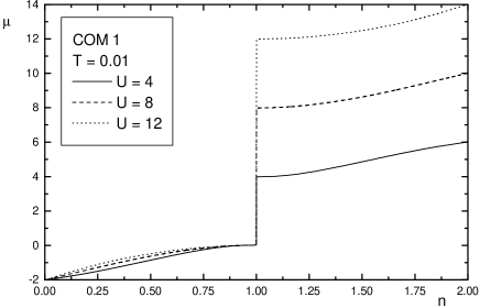
Figure 3: Chemical potential $\mu$ as function of $n$ for $T=0.01$ and $U=4$, $8$ and $12$ (COM 1 solution).

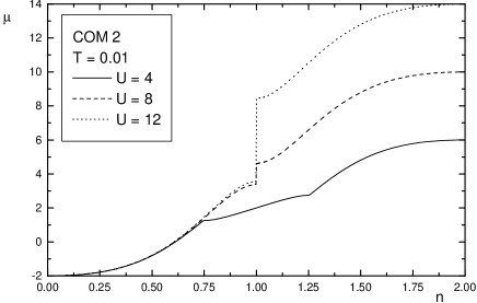
Figure 4: Chemical potential $\mu$ as function of $n$ for $T=0.01$ and $U=4$, $8$ and $12$ (COM 2 solution).

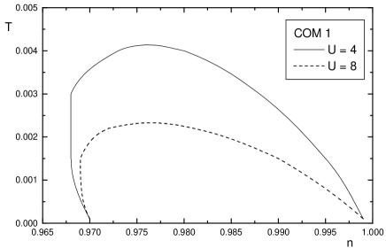
Figure 5: Instability region within the plane $n$-$T$ for $U=4$ and $8$ (COM 1 solution).

The set of self-consistent equations in (22), that determines the internal parameters, admits two distinct solutions. Hereafter, we will call these solutions COM 1 and COM 2. The evolution of the internal parameters with the external ones (i.e., filling, intrasite Coulomb potential and temperature) reveals substantial differences between the two solutions. The $\Delta$ parameter is smaller and much more sensitive to the strength of Coulomb interaction in COM 1 (see Fig. 1). For $n\leq 1$, the $p$ parameter is negative or very small and positive in COM 1, while it is always positive and of the order of the filling in COM 2 see Fig. 2; actually, at half filling and on increasing $U$, $p$ tends to $0$ in COM 1 and to $1$ in COM 2. In COM 1, the chemical potential $\mu$ shows a discontinuity at half filling for any finite value of the Coulomb interaction and a zone of instability (i.e., a negative compressibility) at small doping, temperatures and interaction strength (see Fig. 3). In COM 2, the discontinuity of the chemical potential appears only after a critical value of the Coulomb interaction is reached (see Fig. 4). As we will show in the next section, the absence of the Mott-Hubbard transition, which is a consequence of the mainly negative value of the $p$ parameter, plays a key role in the physics described by the COM 1 solution. The instability of COM  1 can be studied by looking at the compressibility (i.e., $\kappa=\frac{1}{n^{2}}\frac{\partial n}{\partial\mu}$). The instability is confined to a very small region in the plane $(n,T)$. This region does not comprehend half filling (see Fig. 5). For the 2D Hubbard model, which also has two solutions within the framework of the COM, the region of instability is much larger.

III.1 Properties at half filling

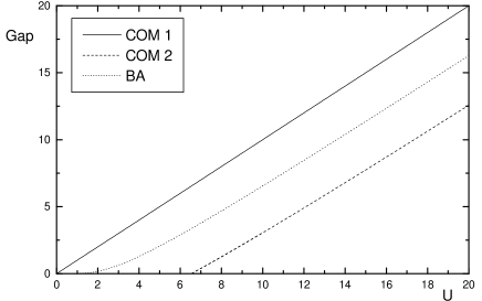
Figure 6: Gap as function of $U$ (COM 1 solution).

Figure 7: Energy spectra $E(k)$ for $T=0$, $n=1$ and $U=7$ and $10$ (COM 1 solution).

Figure 8: Energy spectra $E(k)$ for $T=0$, $n=1$ and $U=7$ and $10$ (COM 2 solution).

Figure 9: $k_{1}$ and $k_{2}$, see definition in the text, as function of $U$ for $T=0$ and $n=1$ (COM 1 solution).

The ground-state properties of the 1D Hubbard model at half filling were exactly derived by Lieb and Wu using the BALieb:68. This exact solution corresponds to an insulating state with short-range antiferromagnetic (AF) correlations for any finite value of $U$. According to this, we will compare the evolution of the gap in the excitation spectrum and the band structure of both solutions with the BA exact results, in order to choose the solution that gives the most consistent physical picture at half filling.

As already mentioned above, within the analysis of the chemical potential, the COM 1 solution presents a gap for any finite value of the Coulomb interaction, in agreement with the BA result, while the COM 2 solution is characterized by a critical value of the Coulomb interaction (i.e., $U_{c}\approx 6.56$) above which a gap opens (see Fig. 6). The rate at which the gap opens in COM 1 coincides with that of the exact solution for $U\geq 4$. The band structure (i.e., the excitation spectrum) of the two solutions is another interesting property to be studied and compared. In fact, many features, more or less anomalous, of both solutions can be easily understood just looking at their spectra. As it can be seen in Fig. 7, the COM 1 solution has a typical AF band pattern (i.e., a quasi-halved Brillouin zone, the first excitation around $k=\pm\frac{\pi}{2}$ and a very narrow bandwidth of the order $J=\frac{4t^{2}}{U}$), in agreement with the BA result. On the contrary, the band structure of the COM 2 solution corresponds to a typically paramagnetic state, with the first hole excitation at $k=\pm\pi$, the first electron excitation at $k=0$ and a bandwidth of the order $8t$ (see Fig. 8). In the figures, the energy is measured with respect to the chemical potential. In particular, while COM 2 has two subbands with both a minimum in $k=0$ and a maximum in $k=\pm\pi$, the COM 1 solution has the upper subband with a maximum in $k=\pm\pi$ and a minimum at $k_{1}=\pm\arccos\theta_{0}$ and the lower subband with a maximum at $k_{2}=\pi-k_{1}$ and a minimum in $k=0$, where

$$\theta_{0}=\frac{p\,U}{2t(1-2p)\sqrt{1-4p}}$$ (68)

For large values of the Coulomb interaction both $k_{1}$ and $k_{2}$ tend to $\frac{\pi}{2}$ since $p$ tends to zero (see Fig. 9). According to this analysis, the width of the subbands and the value of the gap in both solutions can be easily computed. In COM 2, the width of the subbands at half filling is $W=8t\,p$, which tends to $8t$ for large values of the Coulomb interaction, while the gap, above the critical value $U_{c}=4t\sqrt{4p-1}\approx 6.56$, has the expression

$$\Delta E=-8t\,p+\sqrt{U^{2}+16t^{2}(2p-1)^{2}}$$ (69)

On the contrary, in COM 1 the width of the subbands at half filling is

$$W=4t\,p+\frac{1}{2}\sqrt{U^{2}+16t^{2}(2p-1)^{2}}-U\frac{\sqrt{1-4p}}{2(1-2p)}$$ (70)

which tends to $J=\frac{4t^{2}}{U}$ for large values of the Coulomb interaction, while the gap, has the expression

$$\Delta E=\frac{\sqrt{1-4p}}{1-2p}U$$ (71)

Both expressions (i.e., Eqs. (69) and (71)) for the gap tend to $U$ for large values of the Coulomb interaction. It is worth pointing out that, within the two-pole approximation, the $p$ parameter rules the opening of the gap at half filling. In particular, if $p<\frac{1}{4}\left(1+\frac{U^{2}}{16t^{2}}\right)$ we have a gapped solution, because the two subbands have opposite signs for any value of momentum and therefore they do not overlap. This is the case for the COM 1 solution for any value of the Coulomb interaction. For the COM 2 solution we have a gap above the critical value $U_{c}$. Otherwise, we have no gap and the two subbands overlap. In particular, both subbands have negative values for $|k|<\arccos x_{0}$, where $x_{0}=U/U_{c}$.

We can conclude that only COM 1 gives a description of the physics of the half-filled 1D Hubbard model consistent with the exact results obtained by the BA. Therefore, in this section, we will mainly focus on this solution.

III.1.1 Local properties

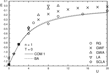
Figure 10: Internal energy $E$ as function of $U$ for $T=0$ and $n=1$ (COM 1 solution).

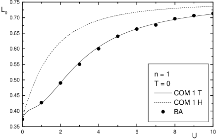
Figure 11: Local magnetization $L_{0}$ as function of $U$ for $T=0$ and $n=1$.

The internal energy, at half filling and zero temperature, can be exactly calculated by means of the BA through Eq. (33). The two relevant limits (i.e., small and large Coulomb interaction) read as follows

$$\lim_{U\rightarrow 0}E= -4\frac{|t|}{\pi}+\frac{1}{4}U+O(\frac{U^{2}}{t})$$

$$\lim_{U\rightarrow\infty}E= -4\frac{t^{2}}{U}\ln 2+O(\frac{t^{4}}{U^{3}})$$ (72)

where $4\ln 2\cong 2.77$. The COM solution exactly agrees with the BA result in the weak-interacting limit, while in the strong-interacting limit, we have

$$\lim_{U\rightarrow\infty}E_{H}^{\emph{COM}1}= -3\frac{t^{2}}{U}+O(\frac{t^{4}}{U^{3}})$$

$$\lim_{U\rightarrow\infty}E_{H}^{\emph{COM}2}= 5\frac{t^{2}}{U}+O(\frac{t^{4}}{U^{3}})$$ (73)

Again, while COM 1 gives a result very close to the BA one, the COM 2 solution is very far in this limit. The internal energy $E$ at half filling and zero temperature, calculated by means of Eq. (30) in the COM 1 solution (i.e., $E_{H}^{\emph{COM}1}$), is shown, as a function of the Coulomb interaction strength, in Fig. 10. The results obtained by means of the BA Shiba:72 and other analytical approachesHirsch:80; Metzner:87; Buzatu:95 are also reported. As we can see, the agreement between COM 1 and BA is excellent. The self-consistent Ladder approximation (SCLA) of Ref. Buzatu:95 shows also a very good agreement for all values of the coupling, but it does not have the correct behaviour for an infinite value of the Coulomb interaction. Moreover, both the Ladder (LA) Buzatu:95 and the Gutzwiller (GWA and GWF) Metzner:87 approximations go to zero at finite $U$, whereas the Renormalization Group (RG)Hirsch:80 has the right asymptotic behaviour for $U\mapsto\infty$, but it does not reproduce the non-interacting limit. The local magnetization $L_{0}$ at half filling and zero temperature as a function of the interaction strength is shown in Fig. 11. We report both the COM results (i.e., $L_{0H}^{\emph{COM}1}$ and $L_{0T}^{\emph{COM}1}$) and the results obtained by means of the BAShiba:72a. $L_{0T}^{\emph{COM}1}$ is in excellent agreement with the exact solution. As one should expect, the electron localization increases with $U$ and for infinite $U$ reaches a saturation (i.e., zero double occupancy and zero kinetic energy). Thus, the 1D itinerant electron system described by the Hubbard chain is equivalent, at half filling and infinite $U$, to the system of localized spins described by the spin-$\frac{1}{2}$ AF Heisenberg model.

III.1.2 Thermodynamic properties

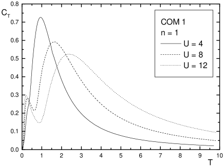
Figure 12: Specific heat $C_{T}$ as function of $T$ for $n=1$ and $U=4$, $8$ and $12$ (COM 1 solution).

Figure 13: Local magnetization $L_{0}$ as function of $T$ for $n=1$ and $U=4$, $8$ and $12$ (COM 1 solution).

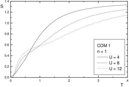
Figure 14: Entropy $S$ as function of $T$ for $n=1$ and $U=4$, $8$ and $12$ (COM 1 solution).

The thermodynamic properties of the Hubbard chain can be evaluated using the BA by means of the finite-temperature formalism developed by Takahashi Takahashi:72.

The specific heat $C_{T}$ at half filling, calculated by means of Eq. 36 in the COM 1 solution (i.e., $C_{T}^{\emph{COM}1}$), is shown in Fig. 12 as a function of the temperature for different values of the Coulomb interaction. By increasing the interaction strength, the single peak present for $U\leq W=4t$ splits in two peaks moving to opposite directions in temperature ($W$ is the non-interacting bandwidth). The low-$T$ feature is due to spin excitations: it is located at $T\sim J$, where $J=\frac{4t^{2}}{U}$ is the magnitude of the induced AF exchange parameter. Such a low-$T$ peak is characteristic of the AF Heisenberg chainBonner:64. This feature is consistent with the AF-like band structure of the COM 1 solution (cfr. Fig. 7). The high-$T$ peak is obviously associated to charge excitations: it moves towards higher temperature as the gap increases with $U$. As $T$ increases, the thermal energy allows the electrons to be excited across the gap. Such a structure of the specific heat, with low- and high- $T$ regions, dominated by spin and charge excitations, respectively, is consistent with the physical picture described by the exact BA solutionShiba:72a; Kawakami:89; Usuki:90; Juttner:98; Deguchi:00 and it also agrees with recent qMC calculations on finite chainsSchulte:96.

In order to get information about the degree of localization of the electrons we have also computed the local magnetization as a function of the temperature. The results are reported in Fig. 13. Let us note that the maximum localization occurs at finite temperature. This is due to the strong antiferromagnetic correlations present at zero temperature. These correlations require a virtual hopping and, therefore, diminish the degree of localization. Only by increasing the temperature we can suppress the antiferromagnetic correlations and increase the localization. Note also that the flat regions at low temperatures end at the same temperature where the local minima develop in $C_{T}$. This further confirms the spin-nature of the low-$T$ peak in the specific heat.

In the temperature evolution of the entropy at half filling, spin and charge degrees of freedom manifest separately in the strong-interacting regime $U\geq W$ (see Fig. 14 where $S_{T}^{\emph{COM}1}$ is calculated by means of Eq. 38 in the COM 1 solution). The low-$T$ region is dominated by spin excitations and the high-$T$ region by particle excitations. The internal energy shows an analogous behavior. The borderline between these two regions can be set at $T\sim t$ in very good agreement with both BA Kawakami:89; Usuki:90 and numericalShiba:72a results. It is worth noting that, in our solution, the entropy shows the correct limiting behavior for high temperatures (i.e., $\lim_{T\rightarrow\infty}S_{T}=2\ln 2\cong 1.39$).

III.1.3 Correlation functions and susceptibilities

Figure 15: Static and uniform charge susceptibility $\chi_{c}$ as function of $T$ (COM 1 solution).

Figure 16: Static and uniform spin susceptibility $\chi_{s}$ as function of $T$ (COM 1 solution).

Figure 17: Spin correlation function $S(r)$ for $T=0$, $n=1$ and $U=4$, $10$ (COM 1 solution).

A quantity which gives information about the evolution of the charge excitations in the system is the charge susceptibility ($\chi_{c}$), which we calculate by means of Eq. (67). This property is shown in Fig. 15 for $n=0.9$ and $n=1$; string theory results are taken from Ref. Deguchi:00. The first thing to note is the strong dependence of $\chi_{c}$ on the particle concentration at low temperatures and for any coupling regime (not shown): the charge susceptibility is strongly enhanced as $n$ approaches half filling, while it goes to zero at $n=1$ as a consequence of the opening of the gap in the charge excitation spectrum. It is worth noticing our good agreement with the practically exact results of qtmJuttner:98. For increasing Coulomb interaction (not shown), the low-temperature enhancement of $\chi_{c}$ in the low doping region is more evident, indicating that the charge excitations are strongly renormalized by the Coulomb interaction near the metal-insulator transition. At higher temperatures, however, $\chi_{c}$ decreases with increasing $U$ regardless of the electron concentrationSanchez:99a.

These are already well-known resultsKawakami:89; Usuki:90 that the approximation considered here is able to reproduce, thus capturing the physics of the charge excitations near the metal-insulator transition. The temperature at which the gap closes due to the thermal excitations is somewhat larger in COM 1 than in the Bethe Ansatz resultsKawakami:89; Usuki:90. This is coherent with the larger value that we obtain for the gap. Also, $\chi_{c}$ is more enhanced near half filling (for instance, at $U=8t$ and $n=0.8$, $\chi_{c,max}^{\emph{COM}1}\sim 0.9$ while $\chi_{c,max}^{BA}\sim 0.25$) because of the faster rate at which the gap opens in our approximation with respect to BA.

Information on the physics of the spin excitations can be extracted from the evolution of the magnetic susceptibility with temperature and Coulomb interaction. We discuss the situation close to half filling. The magnetic susceptibility $\chi_{s}$ is calculated by means of Eq. (60) and its behavior, as a function of the temperature and $U$, is shown in Fig. 16. $\chi_{s}$ presents a peak at low temperatures which moves to lower ones as $U$ increases. It is also worth noticing that $\chi_{s}$ is generally enhanced by $U$. At half filling [not shown], our results indicate a renormalization of the spin excitations, as it is obtained in the case of the charge susceptibility. This behaviour of $\chi_{s}$ for the interacting half-filled chain does not reproduce the BA resultKawakami:89; Usuki:90. According to the exact solution, $\chi_{s}$ should show the same qualitative behaviour regardless of the particle density, because the metal-insulator transition at $n=1$ does not renormalize the spin excitations. Such disagreement between COM 1 and BA is due to the computation of the two-particle Green’s functions within the one-loop approximation. In this approximation, the charge and spin correlation functions have the same spatial dependence (cfr. Eq. (65)), and consequently, gaps in charge or spin sectors will open simultaneously. Therefore, we obtain the same qualitative behaviour for both the charge and spin susceptibility.

This disagreement is also present in the results we have obtained for the spin-spin correlation function (see Fig. 17). It presents a typical paramagnetic behavior (i.e., it is always negative at any finite distance) in contrast with the exact diagonalization resultsShiba:72a; Xu:92 which report short-range antiferromagnetic correlations (i.e., a spin-spin correlation function alternating in sign between sites and rapidly decreasing). Nevertheless, the present approach preserves the $2k_{{\rm F}}$ oscillations for any value of the Coulomb interaction.

III.2 Properties at arbitrary filling

BA predicts a non-magnetic metallic ground state for the 1D Hubbard model at arbitrary filling, with gapless charge and spin excitations Lieb:68. Ground-state properties, like the internal energy, chemical potential and local moment, were studied following Lieb and Wu as a function of the electron density and Coulomb interactionShiba:72; Carmelo:88, mainly in the large-$U$ limit, where analytic expressions could be obtained. By means of the formulation developed by Takahashi for finite temperatures Takahashi:72, some thermal properties at arbitrary filling were also calculatedKawakami:89; Usuki:90. More recently, important single-particle properties, as the spectral function and momentum distribution function, have been evaluated within the BAOgata:90; Qin:96 and by means of numerical techniques, like qMC Xu:92; Sorella:90; Preuss:94. Information on the charge and spin dynamics is the object of the most recent studies on one-dimensional models, with the aim of applying them to real systems. Thus, some authors have analyzed the corresponding two-body correlation functions of the 1D Hubbard model by means of numerical approachesXu:92; Sorella:90, by using the exact BA solutionOgata:90; Schulz:90 or through other analytic approaches, like g-ology Voit:95.

In the following sections we present the results obtained for such quantities within the COM for the Hubbard chain away from half filling. The COM 2 solution is not considered, since, as we have commented above, it does not provide a good description of the system in the case of half filling. Thus, the COM 1 results are compared to the ones available by other systematics. We devote special attention to the quarter-filled case, since it seems to be a relevant particle density for many 1D organic metalsVescoli:98.

III.2.1 Local properties

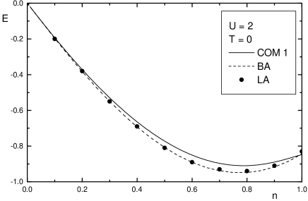
Figure 18: Internal energy $E$ as a function of $n$ for $T=0$ and $U=2$.

Figure 19: Internal energy $E$ as a function of $n$ for $T=0$ and $U=4$.

Figure 20: Chemical potential $\mu$ as a function of $n$ for $T=0$ and $U=2$ and $4$.

Figure 21: Double occupancy $D$ as a function of $U$ for $T=0$ and $n=0.5$ and $0.75$.

The doping dependence of the internal energy, calculated by means of Eq. (30) in the COM 1 solution (i.e., $E_{H}^{\emph{COM}1}$), is shown in Figs. 18 and 19 for two values of the Coulomb interaction. For comparison, we also report the BA resultsShiba:72 and the ladder (LA) and self-consistent ladder (SCLA) approachesHirsch:80; Buzatu:95. COM 1 agrees reasonably with BA, reaching the best agreement at half filling. The ladder approximationBuzatu:95 deviates more and more from the BA as approaching half filling; the self-consistent ladder approximation Buzatu:95 probes excellently at any doping.

The evolution of the chemical potential with the particle density for COM 1 is compared in Fig. 20 with some numerical dataSchulte:96. There is a good agreement over all the range of doping for the higher temperature. The disagreement at the lower temperature can be understood by looking at the size of the gap in COM 1: COM 1 gap is larger than the BA one and forces the chemical potential to assume lower (higher) values than in the BA solution for $n<1$ ($n>1$).

The good agreement with BA, at quarter-filling and for any value of $U$, occurs for the double occupancy too. For other values of filling the agreement is less satisfactory (see Fig. 21).

III.2.2 Thermodynamic properties

Figure 22: $\gamma=C_{H}/T$ as a function of $n$ for $U=8$ and $T=0.01$, $0.05$, $0.1$ and $0.4$ (COM 1 solution).

Figure 23: Filling $n$ as a function of the chemical potential $\mu$ for $U=8$ and $T=0.05$, $1$, $2$ and $4$ (COM 1 solution).

The evolution of the specific heat $C_{H}$ with the particle density is studied for various temperatures in the strong coupling regime. As shown in Fig. 22, $\gamma=C_{H}/T$ has a peak at low densities that simply reflects the shape of the density of states (see discussion on single-particle properties in the next section). As $n$ approaches half filling, another peak develops at low temperatures. This indicates an increasing number of excited states due to the renormalization of the charge fluctuations at the opening of the Mott gap. Let us note that such a peak does not appear in strongly correlated systems which do not have a metal-insulator transition like the 1D electron gas with delta-function interactionsUsuki:89. As one should expect, with increasing temperature, the two peaks merge. COM 1 results for $C_{H}/T$ recover qualitatively those obtained by BA Kawakami:89. There are some quantitative differences, namely: the first peak appears at higher fillings and the double-peak feature survives up to higher temperatures in BA; the peak near half filling is higher in COM 1. This latter difference is expected as the COM 1 gap is larger than the BA one.

To complete the above discussion we show in Fig. 23 the particle density $n$ versus the chemical potential $\mu$ for various temperatures. COM 1 results are compared with the BA ones of Ref. Kawakami:89. The agreement is very good at low temperatures for densities smaller than $0.55$. In the half-filled chain, $T\sim t$ is a relevant temperature as it signs the border between $T$-regions dominated by either spin or charge correlations Shiba:72a; Schulte:96. The agreement between COM 1 and BA at $T\geq t$ is very good for the whole range of filling. Of course, at higher temperatures COM 1 result reaches an excellent agreement with BA since the effect of correlations is completely suppressed.

III.2.3 Single-particle properties

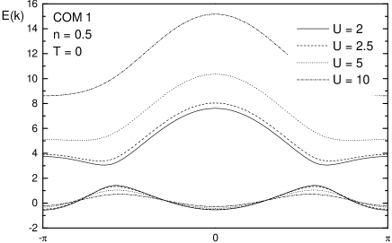
Figure 24: Energy spectra $E(k)$ for $n=0.5$, $T=0$ and $U=2$, $2.5$, $5$ and $10$ (COM 1 solution).

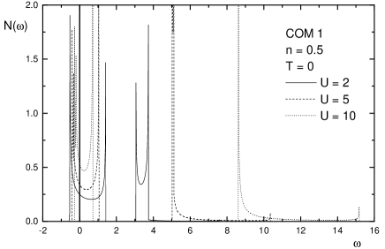
Figure 25: Density of states for $n=0.5$, $T=0$ and $U=2$, $5$ and $10$ (COM 1 solution).

Figure 26: Momentum distribution function in real space $B(r)$ for $n=0.5$, $T=0$ and $U=0$, $2.5$, $5$, $10$ and $30$ (COM 1 solution).

The evolution of the band structure with the interaction strength $U$ is remarkable. Away from half filling the AF-band pattern of the upper Hubbard subband in COM 1 disappears as $U$ increases; the first electron excitations appear at $k=\pm\pi$ and the first hole excitations move slightly away from the half-filling position $k=\pm\pi/2$ (see Fig. 24).

The corresponding density of states is shown in Fig. 25. It is well known that the density of states in the non-interacting case exhibits two van Hove singularities at the edges of the non-interacting band. In the interacting case each of these singularities splits in two since we have two distinct Hubbard subbands. Due to the AF-like band shape, three van Hove singularities appear in each subband leading to the six peaks of the figure. The third structure in the upper subband of Fig. 25 is smoothed because, away from half filling, as $U$ increases the AF-band shape of the excitation spectrum disappears.

As we can deduce from the above results the system, away from half filling, is a conductor for any value of the interaction strength $U$ in agreement with the BA results. Then, a natural question arises: what universality class does this conductor belong to? This is a central issue in the physics of 1D-models.

The momentum distribution function $n(k)$ is a relevant property because from its behavior the Fermi-liquid or non-Fermi liquid nature of the excitations can be inferred. As it is well known, a finite jump in the zero-temperature momentum distribution function at the Fermi momentum $k_{{\rm F}}$ would indicate that the quasiparticle excitations can be described by a Fermi liquid. Some variationalFazekas:88; Yokohama:87, analyticCarmelo:88 and numericalHirsch:84 approaches failed in understanding the nature of the discontinuity. More recently, approaches valid in the weak coupling regime (g-ology and qMC) have found a power-law singularity at $k_{{\rm F}}$ predicting a marginal Fermi-liquid nature away from half fillingSorella:90. The power-law coefficient seems to be an increasing function of $U$ and a decreasing function of the particle density $n$.

The approximation that we use limits the information that can be obtained from the momentum distribution function. Namely, any two-pole approximation has a momentum distribution function with sharp discontinuities at the values of momentum where the Hubbard subbands cross the Fermi level. Despite this strong limitation, the momentum distribution function obtained at quarter filling in COM 1 presents, besides a sharp jump at $k_{{\rm F}},$ another discontinuity near $3k_{{\rm F}}$ . This latter feature is also obtained, as a weak singularity, in BA calculations in the large-$U$ limitOgata:90.

The momentum distribution function in real space obtained in COM 1 is shown in Fig. 26 for various interaction strengths and quarter filling. In the weak coupling regime, the distribution function has nodes at $r=4a,8a,12a,\ldots$ which correspond to an oscillation of wavelength $8a$. Since for these values of interaction and particle density the Fermi momentum is $\frac{\pi}{4}$, this is just a $k_{{\rm F}}$ oscillation. Such an oscillation is also observed by exact diagonalization resultsXu:92 for small $U$. For stronger interactions, a weak incommensurate modulation, in addition to the $k_{{\rm F}}$ oscillation, appears and corresponds to a $3k_{{\rm F}}$ oscillation again in agreement with the exact diagonalization calculationsXu:92. The origin of this $3k_{{\rm F}}$ feature is however not clear. According to other numerical calculationsQin:96 the $3k_{{\rm F}}$ singularity seems to be a finite-size effect and vanishes in the thermodynamic limit. We actually confirm its presence also in the bulk system.

III.2.4 Correlation functions and susceptibilities

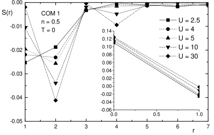
Figure 27: Spin correlation function $S(r)$ for $n=0.5$, $T=0$ and $U=2.5$, $4$, $5$, $10$ and $30$ (COM 1 solution).

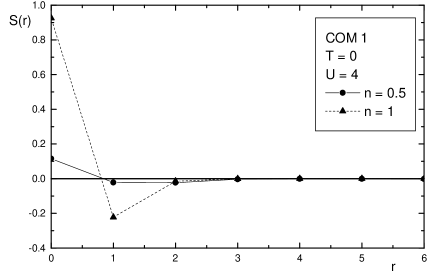
Figure 28: Spin correlation function $S(r)$ for $U=4$, $T=0$ and $n=0.5$ and $1$ (COM 1 solution).

Figure 29: Spin correlation function $S(k)$ for $n=0.5$, $T=0$ and $U=0$, $2$, $4$ and $8$ (COM 1 solution).

Figure 30: Spin susceptibility $\chi_{s}(k)$ for $U=4$, $T=0.001$ and $n=0.99$ on the extended zone (COM 1 solution).

Figure 31: Spin susceptibility $\chi_{s}(k)$ for $U=4$, $T=0.001$ and $n=1$, $0.99$, $0.98$, $0.96$, $0.94$, $0.92$ and $0.9$ (COM 1 solution).

Figure 32: Interband spin susceptibility $\chi^{inter}_{s}(k)$ for $U=4$, $T=0.001$ and $n=1$, $0.99$, $0.98$, $0.96$, $0.94$, $0.92$ and $0.9$ (COM 1 solution).

Figure 33: Static and uniform spin susceptibility $\chi_{s}$ as function of $T$ for $n=0.5$ and $U=2$, $3$ and $4$.

Figure 34: Static and uniform spin susceptibility $\chi_{s}$ as function of $T$ for $U=8$ and $n=0.5$, $0.7$ and $0.9$ (COM 1 solution).

Figure 35: Spin susceptibility $\chi_{s}(k)$ for $n=0.5$, $T=0$ and $U=0$, $2$, $4$ and $10$ (COM 1 solution).

Figure 36: Static and uniform spin susceptibility $\chi_{s}$ as a function of $U$ for $n=0.5$ and $T=1/14.5$.

Figure 37: Static and uniform spin susceptibility $\chi_{s}$ as a function of $T$ for $n=0.5$ and $U=4$.

Figure 38: Normalized spin susceptibility $\chi_{s}(k)\frac{\pi}{\sqrt{2}}$ for $n=0.5$, $U=2$ and $T=0.005$, $1/14.5$, $1/7.25$, $1/4.5$, $1/3.75$ and $1/3$.

The spin correlation function gives information about the spin dynamics of the system. Combining this information with the one obtained from the momentum distribution function, we can analyze how the electron dynamics is affected by the surrounding spins, since the spin configuration is modified when an electron moves to another site. Therefore, the electron motion will depend on how the spin configuration constrains the electron dynamics.

The spin correlation function in real space is evaluated in COM 1 for various interacting regimes and relevant particle densities. The results are shown in Figs. 27 and 28. As we can see, the amplitude of spin correlation increases with $U$ and is smeared out away from half filling. The larger the Coulomb interaction is, the faster the correlations decay. The physical picture that emerges for the half-filled and quarter-filled Hubbard chain is different. At $n=1$ there are strong antiferromagnetic spin correlations that decay very fast (at second neighbor sites they are almost zero). The existence of short-range AF order is also visible in the band spectrum as we previously discussed in detail. For $n=0.5$ these correlations are much weaker and decay more slowly than in the half-filled case. These results agree with the ones described in Ref. Xu:92 using exact diagonalization techniques. In these calculationsXu:92 the spin correlation function has a $2k_{{\rm F}}$ oscillation that is not smeared out away from half filling. Such oscillation is not observed in Figs. 27 and 28 due to the very fast decay of the correlation amplitude, but it appears as a $2k_{{\rm F}}$ feature in the momentum-dependent spin correlation function $S(k)$ (see Fig. 29 and explanation below).

The spin correlation function in $k$ space has been recently studied by means of various approaches. For instance, by qMC in the weak interacting regimeHirsch:83; Imada:89, by means of BA in the strong interacting regimeOgata:90 and for any value of $U$ by exact diagonalization techniqueXu:92. All of them find a very narrow $2k_{{\rm F}}$ peak which is incommensurate away from half filling. These calculations were performed on finite-size systems. A detailed study of the size dependence of $S(2k_{{\rm F}})$ is given in Ref. Ogata:90, where it is shown how the peak narrows and increases with the system size.

The spin-correlation function in $k$ space is shown in Fig. 29 for the COM 1 solution at quarter filling and various interaction strengths. As $U$ increases, an evolution towards a peaked curve at $2k_{{\rm F}}$ is observed, in qualitative agreement with previous calculationsXu:92; Ogata:90; Hirsch:83; Imada:89. We must, however, remark that within the present approach the peak at $2k_{{\rm F}}$ is much broader. At half filling, the height of the $2k_{{\rm F}}$ peak is very much enhanced, in agreement with BA calculations in the large-$U$ limit. The reduction of the $S(2k_{{\rm F}})$ peak as $n$ decreases from half filling is due to the presence of holes moving in the system.

The magnetic or spin susceptibility $\chi_{s}$ gives information about the physics of the spin excitations. This property is calculated by means of Eq. (60) and analyzed as a function of temperature, momentum and interaction.

Close to half filling we have a paramagnetic solution with period $2\pi$, but a strong AF order, with a quasi-halved Brillouin zone, is present (see Fig. 30). When we move away from half filling the central peak opens in two separate peaks (see Fig. 31)). The incommesurability amplitude increases linearly with doping with a coefficient of $\pi/2$ at zero temperature. If we distinguish the intraband and interband contributions we can show that the interband contribution is very little (see Fig. 32). At half filling the susceptibility is strongly reduced and goes to zero at zero temperature: the interband contribution goes much slower to zero with temperature and for the analyzed temperature ($T=0.001$) is the only one present (see Figs. 31 and 32).

Fig. 33 shows the temperature evolution of $\chi_{s}$ for weak and intermediate coupling. Monte Carlo dataNelisse:99 and qtm resultsJuttner:98 are included for comparison. The agreement is good, with a maximum deviation of 15%. We shall note that the position of the maximum does hardly depend on the strength of interaction and is located around $0.2$ (in units of $t$). This indicates that the energy necessary to excite the spin modes does not depend on $U$. Since $U$ is of Coulomb origin and affects the charge degrees of freedom, the $U$-independence of the peak in the spin susceptibility shows that the spin excitations are independent of the charge. This is coherent with a Luttinger liquid description of the quarter-filled Hubbard chain. On the contrary, at half filling the position of the $T$-dependent spin susceptibility does strongly vary with $U$ (see Fig. 16 and Ref. Shiba:72a), indicating the breaking of the Luttinger liquid picture.

Fig. 34 shows the strong coupling spin susceptibility for several particle densities. Once again, COM 1 results at quarter filling are in good agreement with BAKawakami:89; Usuki:90 (see value and position of $\chi_{s}^{{\rm max}}$), whereas it severely disagrees in the case of higher particle-densities.

The low temperature, momentum dependence of the magnetic susceptibility $\chi_{s}(k)$ at quarter filling is shown in Fig. 35 for all coupling regimes. As $U$ increases, the peak moves towards lower $k$, indicating that spin excitations of larger wavelength mostly contribute. Also, two satellite structures appear and increase with $U$. Such structures have their origin in the van Hove singularities of the density of states. They are not observed in qMC studies probably because they exist only at very small temperatures (see Fig. 38).

The static uniform susceptibility is plotted in Figs. 36 and 37 as function of $U$ and $T$, respectively. In Fig. 36 we also report the quantum Monte Carlo dataHirsch:84 and the BA results. The agreement, in particular in the weak coupling regime, is quite good. In Fig. 37 the comparison with the qMC Hirsch:84 and the qtmJuttner:98 results shows: 1) the qMC data do not agree at all with the qtm results, which are practically exact; 2) a good qualitative agreement between COM and qtm at very low temperatures for all three values of Coulomb repulsion $U$( the qtm results present a more pronounced peak) and a very good quantitative agreement at intermediate and high temperatures. Anyway, the position of the peak is very well reproduced confirming once more the capability of the present method to catch the spin energy scale although the retained spin correlations are weaker than what is expected according to the exact and numerical results.

The weak coupling spin susceptibility (normalized to its non-interacting value at $k=0$: $\chi_{s}(0)[U=0]=\frac{\sqrt{2}}{\pi}$, see Eq. 63) is shown in Fig. 38. Despite the simplicity of the one-loop approximation we get a good qualitative agreement with the quantum Monte Carlo dataHirsch:84, as opposed to RPA fits, which need to take different values for the renormalized interaction, as it is remarked in Ref. Nelisse:99. We exactly reproduce the peak at $\pi/2$, which vanishes on increasing temperature, and the asymmetry they found in the intensity between $k=0$ and $k=\pi$.

IV Conclusions

In this paper we have analyzed the adequacy of the COM to describe the physics of correlated electrons in 1D systems; in particular, we studied the 1D Hubbard model. Various physical properties, like ground-state and single-particle properties, the thermodynamics, susceptibilities and some correlation functions, have been calculated and compared to results obtained by means of the Bethe Ansatz, when available, and other analytic and numerical techniques (qMC, GA, SCLA, RG, g-ology).

By considering a two-pole approximation and a paramagnetic state, the model is solved within the COM. Two mathematical solutions (COM 1 and COM 2) are obtained. In the case of half filling an analysis of the parameters and the energy spectra that characterize the solution shows that only COM 1 is consistent with the BA results. Hence, the subsequent properties are discussed only for this solution. The half-filled and arbitrary-filled cases are addressed separately since they lead to different characteristics.

The essential physics of the half-filled Hubbard chain is reproduced satisfactorily by the COM 1 solution. A gap opens for any finite value of the $U$ interaction and the bands show the characteristic AF-like features, with bandwidth of the order of the antiferromagnetic exchange interaction $J=\frac{4t^{2}}{U}$. This indicates, therefore, an insulator with short-range AF correlations, as it is known from the exact BA result. Also, the evolution of the total energy, the double occupancy and the local magnetization with $U$ are in excellent agreement with BA and improves significantly the results of other analytic approaches.

The thermodynamic properties give the following picture. As the interaction strength increases relative to the non-interacting bandwidth $W$ and reaches $U>W=4t$, two energy scales manifest in the system in the form of two peaks in the specific heat. These peaks are located at low ($T\sim J$) and high $T$ and are associated to spin and charge excitations, respectively. The spin nature of the low-$T$ peak in $C_{T}$ is confirmed by the evolution of the local magnetization with temperature. In the strong interacting regime, the spin and charge degrees of freedom also manifest separately in the entropy, where $T\sim t$ is the border between the two regions. This picture agrees qualitatively and quantitatively (position and height of peaks in $C_{T}$ and border between the spin and charge-dominated regions in $S_{T}$) with BA.

The behaviour of the charge excitations near the metal-insulator transition is also very well captured. This can be seen from the analysis of the charge susceptibility $\chi_{c}$ versus $T$ for particle densities approaching $n=1$. The agreement with BA is only qualitative because the faster opening of the gap in COM 1 leads to larger values of $\chi_{c}$.

The physics of the spin excitations, extracted from the evolution of the spin susceptibility $\chi_{s}$, is not properly described. Our results for $\chi_{s}$ indicate, in disagreement with BA, a renormalization of the spin excitations as the system approaches half filling, analogous to what is observed for the charge excitations. This failure is inherent to the one-loop approximation; within the latter gaps in charge and spin sectors open simultaneously since the charge and spin correlation functions have the same spatial dependence.

The basic physics of the arbitrary-filled Hubbard chain is reproduced satisfactorily by the COM 1 solution. In agreement with BA results, we obtain a non-magnetic metal for any coupling regime. Namely, the band spectrum is gapless for any value of $U$, it loses gradually its AF-like characteristics, and the amplitude of the spin correlation function is much reduced in comparison with that obtained at half filling.

Our analysis for arbitrary filling is centered mostly on $n=0.5$ which is relevant to real quasi-1D systems. At this particular filling, low-temperature local quantities like the double occupancy and the chemical potential are in very good agreement with BA results for both weak and strong coupling regimes. The internal energy versus particle density in COM 1 has a reasonable agreement with BA although it is not so good as that of other approaches.

The evolution of the specific heat with particle density reproduces qualitatively the BA results. The $T$-dependent spin susceptibility at quarter filling has a reasonable agreement in the weak and strong coupling regime with quantum Monte Carlo and BA data, respectively.

The momentum distribution function $n(k)$, the correlation functions and the susceptibilities provide information on the universality class this system belongs to and on its charge and spin dynamics.

We can grasp some characteristic features. Namely, the weak singularity at $3k_{{\rm F}}$ obtained in the large-$U$ limit BA calculations at quarter filling would correspond to the discontinuity near $3k_{{\rm F}}$ that is observed in the COM 1 momentum distribution function. This feature would also agree with the $3k_{{\rm F}}$ oscillation of the distribution function in real space $C(r)$ obtained by numerical techniques. The $k_{{\rm F}}$ oscillations of $C(r)$ observed by exact diagonalization calculations are also reproduced in the weak coupling COM 1 results.

The approach manages to grasp the different physics for the half-filled and arbitrary-filled case, in particular quarter filling. By comparing the amplitude of the spin correlation function in real space $S(r)$, we conclude that at quarter filling these correlations are much weaker and decay more slowly than at half filling, in agreement with exact diagonalization results.

The $2k_{{\rm F}}$ singularity of the $k$-dependent spin correlation function $S(k)$ obtained in recent BA and numerical approaches is qualitatively described in COM 1 at quarter filling, where, by increasing $U$, an evolution towards a peak structure in $S(k)$ is observed near $2k_{{\rm F}}$. This peak is much enhanced at half filling, in agreement with BA.

To summarize, when integral properties are addressed (local quantities, thermodynamics, total energy), the COM in the two pole approximation is accurate enough to yield a correct description of the system. The agreement with BA is indeed excellent in the case of half filling and improves the results of other analytical methods which are more lengthy and more complex in many cases. The charge susceptibility is also well described as the charge excitations are dominated by the energy scale set by the opening of the Mott gap, and this is indeed caught by a two-pole approach. However, regarding the spin dynamics the one-loop approximation can only grasp some general physics but it is too simple to investigate it properly. We expect to receive better results whenever we will set up an approximation, for the two-particle propagators, well beyond the one-loop one used here. Anyway, it is worth noting how this simple two-pole approximation is able to catch the spin and charge-dominated energy regions.

Appendix A The 2-pole Approximation

The doublet field (3) satisfies the Heisenberg equation

$$i\frac{\partial}{\partial t}\Psi(i)=J(i)=\left(\begin{array}[c]{l}-\mu\,\xi(i)-4t\left[c^{\alpha}(i)+\pi(i)\right]\\ -(\mu-U)\eta(i)+4t\,\pi(i)\end{array}\right)$$ (74)

where $\pi(i)$ is the composite field

$$\pi(i)=\frac{1}{2}\sigma^{\mu}\,n_{\mu}\,c^{\alpha}(i)+c(i)\left[c^{\dagger\alpha}(i)\,c(i)\right]$$ (75)

In the two-pole approximation we linearize the equation of motion (74) as

$$i\frac{\partial}{\partial t}\Psi(i)\cong\sum_{j}\varepsilon(i,j)\,\Psi(j)$$ (76)

where the energy matrix $\varepsilon(i,j)$ is defined by

$$\varepsilon(i,j)=\sum_{l}\left\langle\left\{J(i),\Psi^{\dagger}(l)\right\}\right\rangle\left\langle\left\{\Psi(l),\Psi^{\dagger}(j)\right\}\right\rangle^{-1}$$ (77)

In the two-pole approximation, by assuming translational invariance, the thermal retarded Green’s function $S\left(k,\omega\right)={\cal F}\left[\left\langle{\cal R}\left[\Psi(i)\,\Psi^{\dagger}(j)\right]\right\rangle\right]$ is given by

$$S\left(k,\omega\right)=\frac{1}{\omega-\varepsilon(k)}I(k)$$ (78)

where $\varepsilon(k)={\cal F}\left[\varepsilon(i,j)\right]$ is the energy matrix in momentum space and $I(k)={\cal F}\left\langle\left\{\Psi(i),\Psi^{\dagger}(j)\right\}\right\rangle$ is the normalization matrix.