Correlated quantum measurement of a solid-state qubit

Abstract

We propose a solid-state experiment to study the process of continuous quantum measurement of a qubit state. The experiment would verify that an individual qubit stays coherent during the process of measurement (in contrast to the gradual decoherence of the ensemble-averaged density matrix) thus confirming the possibility of the qubit purification by continuous measurement. The experiment can be realized using quantum dots, single-electron transistors, or SQUIDs.

The impressive advantages promised by quantum computing [1] have revived the interest to the fundamental quantum effects in simple objects: two-level systems, which in this context are nowadays called qubits. In this paper we address the problem of continuous measurement of a qubit state having in mind a solid-state realization of the setup.

Among the numerous proposals of quantum computers, the solid-state realizations (see, e.g. Refs. [2, 3, 4, 5]) look more promising because of better controllability of qubit parameters and inter-qubit couplings. However, the qubit measurement in this case is not as straightforward as in typical optical experiments where the single photon just “clicks” the detector. The reason is finite (and typically weak) coupling with a solid-state detector and finite intrinsic noise of the detector. As a result, the measurement cannot be done instantaneously, and so the collapse postulate of the “orthodox” quantum mechanics [6] cannot be applied directly. Instead, the quantum measurement should be considered as a continuous process.

There are two main theoretical approaches to the continuous quantum measurements. One approach (which dominates in solid-state physics and so can be called “conventional”) is based on the theory of interaction with dissipative environment [7, 8]. Taking trace over the numerous degrees of freedom of the detector, it is possible to obtain the gradual evolution of the density matrix of the measured system from the pure initial state to the incoherent statistical mixture, thus describing the measurement process. Since the procedure implies the averaging over the ensemble, the final equations of this formalism are deterministic and can be derived from the Schrödinger equation alone, without any notion of the state collapse.

The other approach (see, e.g., Refs. [9, 10, 11, 12, 13, 14]) is closer to the collapse viewpoint and describes the stochastic evolution of an individual quantum system due to continuous measurement. This evolution obviously depends on a particular measurement result and is usually called selective or conditional quantum evolution. Depending on the details of the studied measurement setup and applied formalism, different authors [9, 10, 11, 12, 13, 14] discuss quantum trajectories, quantum state diffusion, stochastic evolution of the wavefunction, quantum jumps, stochastic Schrödinger equation, complex Hamiltonian, method of restricted path integral, Bayesian formalism, etc. The theory of selective quantum evolution was only recently introduced into the context of solid-state mesoscopics [14, 15]. In particular, it was shown that the continuous measurement of an individual qubit does not lead to gradual decoherence (in contrast to the conventional result for the ensemble), instead, the measurement can lead to gradual purification of the qubit density matrix.

Since the concept is still considered controversial, the experimental check is quite important. In this paper we propose an experiment which can be realized using three possible setups available for present-day technology: double-quantum-dot qubit measured by quantum point contact [16], qubit based on single-Cooper-pair box measured by single-electron transistor [17], or SQUID-based qubit measured by another SQUID [18, 19].

Let us start with reviewing the result of the conventional formalism for the continuous measurement (Fig. 1) of a qubit state (see, e.g. recent publications [16, 20, 21, 22, 23, 24, 25]). For the qubit characterized by the standard Hamiltonian ${\cal H}_{QB}=(\varepsilon/2)(c_{1}^{\dagger}c_{1}-c_{2}^{\dagger}c_{2})+H(c_{1}^{\dagger}c_{2}+c_{2}^{\dagger}c_{1})$ in the basis defined by coupling with the detector, the evolution of qubit density matrix $\rho$ is given by equations

$$\dot{\rho}_{11}=-\dot{\rho}_{22}=-2H\mbox{Im}\rho_{12},$$ (1)

$${\dot{\rho}}_{12}=\imath\varepsilon\rho_{12}+\imath H(\rho_{11}-\rho_{22})-\Gamma\rho_{12},$$ (2)

where the continuous measurement is described by the dephasing rate $\Gamma$, which was calculated for different models in Refs. [16, 20, 21, 22, 23, 24, 25].

These equations do not depend on the detector output because they represent the result of ensemble averaging, including the averaging over the measurement result. To study the evolution of an individual qubit let us denote the noisy detector signal as $I(t)$ (assuming current for definiteness). Two “localized” qubit states 1 and 2 correspond to average detector currents $I_{1}$ and $I_{2}$ which by assumption do not differ much, $\Delta I\equiv I_{1}-I_{2}\ll I_{0}\equiv(I_{1}+I_{2})/2$. (This assumption of “weakly responding” detector [14] allows us to use the linear response theory and also Markov approximation if the processes in the detector are much faster than the qubit evolution.) Intrinsic noise of the detector signal is characterized by the spectral density $S$ which is frequency-independent in the range of interest. The noise determines the typical measurement time $t\sim S/(\Delta I)^{2}$ necessary to distinguish between states 1 and 2, and thus defines the timescale of the selective evolution of the qubit density matrix $\rho(t)$.

     

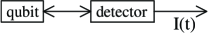
FIG. 1.: Schematic of a qubit continuously measured by a detector with output signal $I(t)$.

Within the Bayesian formalism [14] the selective evolution is described by equations

$$\dot{\rho}_{11}= -2H\mbox{Im}\rho_{12}+(2\Delta I/S)\,\rho_{11}\rho_{22}[I(t)-I_{0}],$$ (3)

$${\dot{\rho}}_{12}= \imath\varepsilon\rho_{12}+\imath H(\rho_{11}-\rho_{22})$$ (5)

$$-(\Delta I/S)\,(\rho_{11}-\rho_{22})[I(t)-I_{0}]\,\rho_{12}-\gamma\,\rho_{12},$$

where the dephasing $\gamma=\Gamma-(\Delta I)^{2}/4S\geq 0$ is now due to the contribution from “pure environment” only. In particular, $\gamma=0$ if the qubit is measured by symmetric quantum point contact, since in this case $\Gamma=(\Delta I)^{2}/4S$ (see Refs. [20, 21, 16, 25]). We will call such detector an ideal detector, $\eta=1$, where $\eta\equiv 1-\gamma/\Gamma$ is the ideality factor. In contrast, the single-electron transistor [26] in the operation point far outside the Coulomb blockade range is a significantly nonideal detector [24], $\eta\ll 1$; however, $\eta$ becomes comparable to unity when the current is mostly due to cotunneling processes [27]. The SQUID is an ideal detector when its sensitivity is quantum-limited [28, 29].

Eqs. (3)–(5) allow us to calculate the evolution of qubit density matrix $\rho$ if the detector output $I(t)$ is known from a particular experiment. To simulate the measurement we can use the replacement [14]

$$I(t)-I_{0}\,=\,\Delta I(\rho_{11}-\rho_{22})/2+\xi(t),$$ (6)

where the random process $\xi(t)$ has zero average and “white” spectral density $S_{\xi}=S$. One can check that averaging of Eqs. (3)–(5) over all possible measurement results [i.e. over random contribution $\xi(t)$] reduces them to Eqs. (1)–(2). Notice that the stochastic equations are written in Stratonovich form which preserves the usual calculus rules, while averaging is more straightforward in Itô form [30].

As follows from Eqs. (3)–(5), if a qubit with initially pure state, $|\rho_{12}(0)|^{2}=\rho_{11}(0)\rho_{22}(0)$, is measured by an ideal detector, then its density matrix $\rho(t)$ stays pure during the measurement process. Even if initial state is a statistical mixture, $\rho(t)$ is gradually purified during the measurement [14].

The predictions of the Bayesian formalism can be checked experimentally, however, it is not quite simple at the present-day level of solid-state technology. The direct experiment was discussed in Ref. [14]. The idea was to perform the measurement by almost ideal detector during some finite time $\tau$, record the detector output $I(t)$, use Eqs. (3)–(5) to calculate $\rho(\tau)$ and then check the calculated value. This check can be done by changing qubit parameters $\varepsilon$ and $H$ in a way to ensure $\rho_{11}=1$ at some specified moment of time, that can be measured by the detector switched on again. Since for coherent evolution the qubit can be placed with 100% certainty in the state 1 only if the wavefunction is known precisely, such check (repeated many times) verifies that $\rho(\tau)$ is pure and coincides with the calculated value.

Unfortunately, this experiment would require very fast recording of $I(t)$. Since the expected coherence time is on the order of 10–100 ns at most (see, e.g. [17]), the bandwidth of the detector signal coming out of the cryostat should be at least 1 GHz, that is very difficult experimentally. Another proposed experiment [25, 27] is to measure the spectral density of the quantum coherent oscillations and check the predicted maximal peak-to-pedestal ratio of 4. Such an experiment may be easier to realize (because the basic spectral analysis can be done on-chip inside the cryostat), however, it would not prove unambiguously the Bayesian formalism, since an alternative interpretation of the result is possible [27].

   

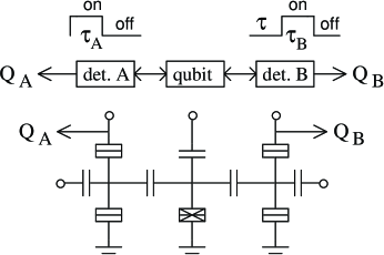
FIG. 2.: Schematic of two-detector correlation experiment using Cooper-pair box and two single-electron transistors.

Here we propose an experiment which is even easier to realize, and which can test the Bayesian formalism (3)–(5). The main idea is to use two detectors ($A$ and $B$) connected to the same qubit (Fig. 2). The detectors are switched on for short periods of time by two shifted in time voltage pulses (one for each detector) with durations $\tau_{A}$ and $\tau_{B}$, supplied from the outside. The output signal from the detector $A$ is the total charge $Q_{A}=\int_{0}^{\tau_{A}}I_{A}(t)\,dt$ passed during the measurement period. Similarly, the output from the detector $B$ is $Q_{B}=\int_{\tau}^{\tau+\tau_{B}}I_{B}(t)\,dt$, where $\tau$ is the time shift between pulses. If the measurement by the detector $A$ changes the qubit density matrix, it will affect the result of measurement $B$. Repeating the experiment many times (with the same initial qubit state) we can obtain the probability distribution $P(Q_{A},Q_{B}|\tau)$ of different outcomes, which contains the information about the effect of the quantum measurement on the qubit density matrix. In comparison with previous suggestions, the advantage of this correlation experiment is that the wide signal bandwidth is required only for input pulses (that is relatively simple) while the outputs are essentially low frequency signals. The experiment can be called “Bell-type” because of some similarity with the famous proposal of Ref. [31].

Fig. 2 shows the realization of the experiment using single-electron transistors (two small tunnel junctions in series [26]) as detectors. Qubit is realized by the Cooper-pair box [32, 17] so that the electric charge of the central island can be in coherent combination of two discrete charge states. Another similar setup is two quantum point contacts measuring the charge state of a double-quantum-dot qubit. One more setup is the 3-SQUID experiment in which the qubit is realized by one SQUID while two other SQUIDs are in the detecting regime. For definiteness we will consider the realization of Fig. 2.

The conventional formalism (1)–(2) does not give any explicit predictions for the resulting probability distribution $P(Q_{A},Q_{B}|\tau)$. However, it implies the absence of correlations between $\rho(t)$ and $I(t)$, so for example the average result of the second measurement $\overline{Q}_{B}(Q_{A},\tau)\equiv\int Q_{B}P(Q_{A},Q_{B}|\tau)\,dQ_{B}$ should not depend on $Q_{A}$. The Bayesian formalism (3)–(5) makes the different prediction: $\overline{Q}_{B}$ does depend on $Q_{A}$.

For simplicity let us assume symmetric qubit, $\varepsilon=0$, which is initially in the ground state, $\rho_{11}=\rho_{22}=\rho_{12}=0.5$, and also assume relatively strong coupling between the qubit and detectors, $(\Delta I_{A})^{2}/HS_{A}\gg 1$, $(\Delta I_{B})^{2}/HS_{B}\gg 1$ (subscripts $A$ and $B$ correspond to two detectors), so that we can neglect the qubit evolution due to finite $H$ during the measurement periods $\tau_{A}$ and $\tau_{B}$, which are assumed to be on the order of $S_{A,B}/(\Delta I_{A,B})^{2}$. Then from Eqs. (3)-(5) if follows that the first measurement only “partially” localizes the qubit state and after obtaining the result $Q_{A}$ from the first measurement the qubit density matrix is

$$2\rho_{11}(\tau_{A})-1=\tanh\frac{(Q_{A}-\tau_{A}I_{2A})^{2}-(Q_{A}-\tau_{A}I_{1A})^{2}}{2S_{A}\tau_{A}}\,,$$ (7)

$$\rho_{12}(\tau_{A})=[\rho_{11}(\tau_{A})\,\rho_{22}(\tau_{A})]^{1/2}\exp(-\gamma_{A}\tau_{A})\,,$$ (8)

where Eq. (7) is actually the classical Bayes formula which was used in Ref. [14] to derive the formalism (3)–(5). [The probability to get $Q_{A}$ has the distribution $P(Q_{A})=(p_{1}+p_{2})/2$ where $p_{i}=(\pi S_{A}\tau_{A})^{-1/2}\exp(-(Q_{A}-\tau_{A}I_{iA})^{2}/S_{A}\tau_{A})$.] The qubit performs the free evolution during the time $\tau-\tau_{A}$ between measurements (here we neglect $\tau_{A}\ll\tau$) and the average result of the second measurement $\overline{Q}_{B}=\tau_{B}(I_{2B}+\rho_{11}(\tau)\Delta I_{B})$ depends on $Q_{A}$ in the following way (Fig. 3a):

$$\delta_{B}= \frac{1}{2}\tanh\frac{(Q_{A}-\tau_{A}I_{2A})^{2}-(Q_{A}-\tau_{A}I_{1A})^{2}}{2S_{A}\tau_{A}}$$ (10)

$$\times\frac{2H}{\Omega}\cos\left(\Omega\tau-\arcsin\frac{\gamma_{f}}{4H}\right)\exp(-\gamma_{f}\tau/2)\,,$$

where $\delta_{B}\equiv(\overline{Q}_{B}-\tau_{B}I_{0B})/\tau_{B}\Delta I_{B}$, $\gamma_{f}$ is the dephasing with both detectors switched off, and $\Omega=(4H^{2}-\gamma_{f}^{2}/4)^{1/2}$ is the frequency of quantum oscillations (underdamped case is assumed). Notice that $\delta_{B}$ changes sign together with the sign of $Q_{A}-\tau_{A}I_{0A}$, while the phase of oscillations is a piece-constant function of $Q_{A}$.

    

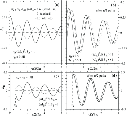
FIG. 3.: The normalized average result $\delta_{B}$ of the second measurement for several selected results $Q_{A}$ of the first measurement, as a function of the time $\tau$ between measurements. Panels (a)–(b) are for strong coupling and panels (c)–(d) for moderate coupling between the qubit and detectors (other parameters are the same). The calculations are done by Bayesian formalism while the conventional formalism does not predict any nontrivial dependence.

The dependence becomes quite different if the $\pi/2$ pulse is applied to the qubit immediately after the first measurement, that multiplies $\rho_{12}(\tau_{A})$ given by Eq. (8) by the imaginary unit. In this case (Fig. 3b)

$$\delta_{B} =A\sin(\Omega\tau+\arcsin z/A)\exp(-\gamma_{f}\tau/2)\,,$$ (12)

$$A=[(z^{2}+y^{2}-yz\gamma_{f}/2H)/(1-\gamma_{f}^{2}/16H^{2})]^{1/2},$$

where $z=\rho_{11}(\tau_{A})-1/2$ and $y=\mbox{Im}\rho_{12}(\tau_{A}+0)=\mbox{Re}\rho_{12}(\tau_{A}-0)$ are given by Eqs. (7)–(8). This expression considerably simplifies for weak dephasing, $\gamma_{A}\tau_{A}\ll 1$ and $\gamma_{f}\ll H$, when

$$\delta_{B}=\frac{1}{2}\sin[\Omega\tau+\arcsin(2\rho_{11}(\tau_{A})-1)]\exp(-\frac{\gamma_{f}\tau}{2}).$$ (13)

In contrast to Eq. (10) now the phase of oscillations $\delta_{B}(\tau)$ depends on the result $Q_{A}$ of the first measurement, while the amplitude is maximal possible and independent of $Q_{A}$. This fact is very important since it proves that after the first measurement (by an ideal detector) the qubit remains in the pure state for any result $Q_{A}$. This state depends on $Q_{A}$ and is not one of the localized states as somebody could naively expect. [Notice that Eq. (10) can in principle be interpreted in terms of such “classical” localization, as indicated by its independence on $\eta_{A}$.]

In a realistic experimental situation the assumption of strong coupling with detectors may be inapplicable. In this case the full probability distribution $P(Q_{A},Q_{B}|\tau)$ as well as the dependence $\overline{Q}_{B}(Q_{A},\tau)$ can be calculated numerically using Eqs. (3)–(6). The results of these calculations for $(\Delta I_{A})^{2}/HS_{A}=(\Delta I_{B})^{2}/HS_{B}=1$ are shown in Figs. 3c and 3d. Weak coupling as well as the nonideality of the detectors decrease the correlation between the results of two measurements, however, for moderate values of the coupling and nonideality the correlation is still significant.

The successful experimental demonstration of the correlation and quantitative agreement with the results of the Bayesian formalism would prove the validity of this formalism and therefore prove its other predictions. Besides the clarification of the relation between the measurement result and qubit evolution, the important for practice prediction is the gradual qubit purification due to continuous measurement which can be useful for a quantum computer.

All quantum algorithms require the supply of “fresh” qubits with well-defined initial states. This supply is not a trivial problem since the qubit left alone for some time deteriorates due to interaction with environment. The usual idea is to use the ground state which should be eventually reached and does not deteriorate. However, to speed up the qubit initialization we need to increase the coupling with environment that should be avoided. The other possible idea is to perform the projective measurement after which the state becomes well-defined. However, in the realistic case the coupling with the detector is finite that makes projective measurements impossible. Here we propose a different way: to tune qubit continuously in order to overcome the dephasing due to environment and so keep qubit “fresh”.

   

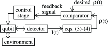
FIG. 4.: Schematic of the continuous qubit purification using the quantum feedback loop.

The idea of such state purification is shown in Fig. 4. The qubit is continuously measured by weakly coupled detector, and the detector signal is plugged into Eqs. (3)–(5) which allow us to monitor the evolution (in particular, due to interaction with environment) of qubit density matrix $\rho_{ij}(t)$. This evolution is compared with the desired evolution and the difference is used to generate the feedback signal which controls the qubit parameters $H$ and $\varepsilon$ in order to reduce the difference with the desired qubit state. We have performed the Monte-Carlo simulation of the qubit purification by feedback loop (in the regime of well-pronounced quantum oscillations) and found strong suppression of the qubit dephasing due to environment in the case when the dephasing rate $\gamma$ is comparable or weaker than the “measurement rate” $(\Delta I)^{2}/4S$.

In conclusion, we have proposed the Bell-type experiment which can test the Bayesian formalism predictions for the evolution of an individual qubit due to continuous quantum measurement. The next (and much more difficult) step is the experimental realization of the qubit purification using quantum feedback loop.

The author thanks L. P. Rokhinson, D. V. Averin, M. H. Devoret, C. M. Marcus, and K. K. Likharev for useful discussions.

REFERENCES

- [1] C. Bennett, Phys. Today, Oct. 1995, 24 (1995).
- [2] B. E. Kane, Nature 393, 133 (1998).
- [3] D. V. Averin, Solid State Comm. 105, 659 (1998).
- [4] Yu. Makhlin, G. Schön, and A. Shnirman, Nature 398, 305 (1999).
- [5] J. E. Mooij, T. P. Orlando, L. Levitov, L. Tian, C. H. van der Wal, and S. Lloyd, Science 285, 1036 (1999).
- [6] J. von Neumann, Mathematical Foundations of Quantum Mechanics (Princeton Univ. Press, Princeton, 1955).
- [7] A. O. Caldeira and A. J. Leggett, Ann. Phys. (N.Y.) 149, 374 (1983).
- [8] W. H. Zurek, Phys. Today, 44 (10), 36 (1991).
- [9] N. Gisin, Phys. Rev. Lett. 52, 1657 (1984).
- [10] H. J. Carmichael, An open system approach to quantum optics, Lecture notes in physics (Springer, Berlin, 1993).
- [11] M. J. Gagen, H. M. Wiseman, and G. J. Milburn, Phys. Rev. A 48, 132 (1993).
- [12] M. B. Plenio and P. L. Knight, Rev. Mod. Phys. 70, 101 (1998).
- [13] M. B. Mensky, Phys. Usp. 41, 923 (1998).
- [14] A. N. Korotkov, Phys. Rev. B 60, 5737 (1999).
- [15] A. N. Korotkov, Physica B 280, 412 (2000).
- [16] E. Buks, R. Schuster, M. Heiblum, D. Mahalu, and V. Umansky, Nature 391, 871 (1998); D. Sprinzak, E. Buks, M. Heiblum, and H. Shtrikman, Phys. Rev. Lett. 84, 5820 (2000).
- [17] Y. Nakamura, Yu. A Pashkin, and J. S. Tsai, Nature 398, 786 (1999).
- [18] J. R. Friedman, V. Patel, W. Chen, S. K. Tolpygo, and J. E. Lukens, Nature 406, 43 (2000); S. Han, J. Lapointe, and J. E. Lukens, Phys. Rev. Lett. 66, 810 (1991).
- [19] C. H. van der Wal, A. C. J. ter Haar, F. K. Wilheim, R. N. Schouten, C. J. P. M. Harmans, T. P. Orlando, S. Lloyd, and J. E. Mooij, to be published.
- [20] S. A. Gurvitz, Phys. Rev. B 56, 15215 (1997); quant-ph/9808058.
- [21] I. L. Aleiner, N. S. Wingreen, and Y. Meir, Phys. Rev. Lett. 79, 3740 (1997).
- [22] Y. Levinson, Europhys. Lett. 39, 299 (1997).
- [23] L. Stodolsky, Phys. Lett. B 459, 193 (1999).
- [24] A. Shnirman and G. Schön, Phys. Rev B 57, 15400 (1998).
- [25] A. N. Korotkov and D. V. Averin, e-print cond-mat/0002203.
- [26] D. V. Averin and K. K. Likharev, in Mesoscopic Phenomena in Solids, edited by B. L. Altshuler, P. A. Lee, and R. A. Webb (Elsevier, Amsterdam, 1991), p. 173.
- [27] A. N. Korotkov, e-print cond-mat/0003225.
- [28] V. V. Danilov, K. K. Likharev, and A. B. Zorin, IEEE Trans. Magn. MAG-19, 572 (1983).
- [29] D. V. Averin, e-print cond-mat/0004364.
- [30] B. Øksendal, Stochastic differential equations (Springer, Berlin, 1992).
- [31] J. S. Bell, Physics 1, 195 (1964).
- [32] P. Lafarge, P. Joyez, D. Esteve, C. Urbina, and M. H. Devoret, Phys. Rev. Lett. 70, 994 (1993).