We present exact calculations of partition function $Z$ of the $q$-state Potts model with next-nearest-neighbor spin-spin couplings, both for the ferromagnetic and antiferromagnetic case, for arbitrary temperature, on $n$-vertex strip graphs of width $L_{y}=2$ of the square lattice with free, cyclic, and Möbius longitudinal boundary conditions. The free energy is calculated exactly for the infinite-length limit of these strip graphs and the thermodynamics is discussed. Considering the full generalization to arbitrary complex $q$ and temperature, we determine the singular locus ${\cal B}$ in the corresponding ${\mathbb{C}}^{2}$ space, arising as the accumulation set of partition function zeros as $n\to\infty$.

1 Introduction

The $q$-state Potts model has served as a valuable model for the study of phase transitions and critical phenomena [1, 2]. On a lattice, or, more generally, on a (connected) graph $G$, at temperature $T$, this model is defined by the partition function

$$Z(G,q,v)=\sum_{\{\sigma_{n}\}}e^{-\beta{\cal H}}$$ (1.1)

with the (zero-field) Hamiltonian

$${\cal H}=-J\sum_{\langle ij\rangle}\delta_{\sigma_{i}\sigma_{j}}$$ (1.2)

where $\sigma_{i}=1,...,q$ are the spin variables on each vertex $i\in G$; $\beta=(k_{B}T)^{-1}$; and $\langle ij\rangle$ denotes pairs of adjacent vertices. The graph $G=G(V,E)$ is defined by its vertex set $V$ and its edge (=bond) set $E$; we denote the number of vertices of $G$ as $n=n(G)=|V|$ and the number of edges of $G$ as $e(G)=|E|$. We use the notation

$$K=\beta J\ ,\quad a=u^{-1}=e^{K}\ ,\quad v=a-1$$ (1.3)

so that the physical ranges are (i) $a\geq 1$, i.e., $v\geq 0$ corresponding to $\infty\geq T\geq 0$ for the Potts ferromagnet, and (ii) $0\leq a\leq 1$, i.e., $-1\leq v\leq 0$, corresponding to $0\leq T\leq\infty$ for the Potts antiferromagnet. One defines the (reduced) free energy per site $f=-\beta F$, where $F$ is the actual free energy, via

$$f(\{G\},q,v)=\lim_{n\to\infty}\ln[Z(G,q,v)^{1/n}]\ .$$ (1.4)

where we use the symbol $\{G\}$ to denote $\lim_{n\to\infty}G$ for a given family of graphs.

Let $G^{\prime}=(V,E^{\prime})$ be a spanning subgraph of $G$, i.e. a subgraph having the same vertex set $V$ and an edge set $E^{\prime}\subseteq E$. Then $Z(G,q,v)$ can be written as the sum [3]-[5]

$$Z(G,q,v) = \sum_{G^{\prime}\subseteq G}q^{k(G^{\prime})}v^{e(G^{\prime})}$$ (1.5)

$$= \sum_{r=k(G)}^{n(G)}\sum_{s=0}^{e(G)}z_{rs}q^{r}v^{s}$$ (1.8)

where $k(G^{\prime})$ denotes the number of connected components of $G^{\prime}$ and $z_{rs}\geq 0$. Since we only consider connected graphs $G$, we have $k(G)=1$. The formula (1.5) enables one to generalize $q$ from ${\mathbb{Z}}_{+}$ to ${\mathbb{R}}_{+}$ (keeping $v$ in its physical range). This generalization is sometimes denoted the random cluster model [5]; here we shall use the term “Potts model” to include both positive integral $q$ as in the original formulation in eqs. (1.1) and (1.2), and the generalization to real (or complex) $q$, via eq. (1.5). The formula (1.5) shows that $Z(G,q,v)$ is a polynomial in $q$ and $v$ (equivalently, $a$) with maximum and minimum degrees indicated in eq. (1.8). The Potts model partition function on a graph $G$ is essentially equivalent to the Tutte polynomial [6]-[10] and Whitney rank polynomial [4], [2], [11]-[13] for this graph, as was discussed in [15] and is briefly noted in the appendix of this paper.

In this paper we shall present exact calculations of the Potts model partition function for strips of the square lattice with next-nearest-neighbor (NNN) spin-spin interactions. Specifically, we consider strips with width $L_{y}=2$ vertices and arbitrarily great length $L_{x}$ with various boundary conditions. To avoid increasing the number of parameters, we take the nearest-neighbor and next-nearest-neighbor coupling strengths to be equal. This study is a natural continuation of our previous analogous calculations for strips of the square and triangular lattices [14, 15, 16], and the reader is referred to these papers for background and further references (see also [17, 18]). We envision the strip as being formed by starting with a ladder graph, i.e. a $2\times L_{x}$ strip of the square lattice, and then adding an edge joining the lower left and upper right vertices of each square, and an edge joining the upper left and lower right vertices of each square (these two added edges do not intersect each other). Following our previous papers [19, 20], we shall denote this lattice as $sq_{d}$, where the subscript $d$ refers to the added diagonal bonds for each square. The Potts model with NNN spin-spin couplings on the square lattice and strips thereof can equivalently be considered as the Potts model with nearest-neighbor couplings on the $sq_{d}$ lattice with these diagonal bonds present. For our strip calculations, we take the longitudinal (transverse) direction on the strip to be the horizontal, $x$ (vertical, $y$) direction, respectively. We use free transverse boundary conditions and consider free, periodic (= cyclic), and Möbius longitudinal boundary conditions. As we showed before [20], for a given value of $L_{x}=m$, the $L_{y}=2$ cyclic $sq_{d}$ strip graph is identical to the corresponding strip with Möbius boundary conditions; hence, we shall refer to them both as $L_{m}=sq_{d}((L_{y}=2)_{m},FBC_{y},(T)PBC_{x})$, where the $L$ here stands for “ladder” (with diagonal bonds added). The open strip will be denoted $S_{m}$. Following our labelling conventions in [21, 22], $L_{x}=m+1$ edges for an open strip $S_{m}$ and $L_{x}=m$ edges for the cyclic/Möbius strip $L_{m}$. One has $n(S_{m})=2(m+2)$, $n(L_{m})=2m$, $e(S_{m})=6+5m$, and $e(L_{m})=5m$. Each vertex on the cyclic/Möbius strip $L_{m}$ has degree (coordination number) $\Delta=5$; this is also true of the interior vertices on the open strip $S_{m}$, while the corner vertices have $\Delta=3$. Hence, the cyclic/Möbius strips $L_{m}$ are $\Delta$-regular graphs with $\Delta=5$, where a $\Delta$-regular graph is defined as one in which each vertex has the same degree, $\Delta$. For the infinite $sq_{d}$ lattice, $\Delta=8$. Note that, regarded as graphs, the cyclic/Möbius strips of the $sq_{d}$ lattice considered here, like the full 2D $sq_{d}$ lattice, are nonplanar (except for $L_{m}$ with $m=1,2$). In contrast, the open strips $S_{m}$ of the $sq_{d}$ lattice are planar graphs.

One interesting special case is provided by the zero-temperature Potts antiferromagnet. In general, for sufficiently large $q$, on a given lattice or graph $G$, the Potts antiferromagnet exhibits nonzero ground state entropy (without frustration). This is equivalent to a ground state degeneracy per site (vertex), $W>1$, since $S_{0}=k_{B}\ln W$. The $T=0$ (i.e., $v=-1$) partition function of the above-mentioned $q$-state Potts antiferromagnet (PAF) on $G$ satisfies

$$Z(G,q,-1)=P(G,q)$$ (1.9)

where $P(G,q)$ is the chromatic polynomial (in the variable $q$) expressing the number of ways of coloring the vertices of the graph $G$ with $q$ colors such that no two adjacent vertices have the same color [3, 11, 23, 24]. The minimum number of colors necessary for this coloring is the chromatic number of $G$, denoted $\chi(G)$. We have

$$W(\{G\},q)=\lim_{n\to\infty}P(G,q)^{1/n}\ .$$ (1.10)

There are several motivations for the present study. Clearly, new exact calculations of Potts model partition functions are of value in their own right. A specific motivation is that this study provides exact results that reveal the effects of next-nearest-neighbor spin-spin interactions on the properties of the Potts model. It is of considerable physical interest what these effects are, since models with strictly nearest-neighbor interactions are only an approximation (albeit often a good one) to nature. For ferromagnetic spin-spin interactions ($J>0$), the addition of (ferromagnetic) NNN interactions clearly enhances the tendency, at a given temperature, toward ferromagnetic ordering. For antiferromagnetic (AF) spin-spin interactions ($J<0$), the effect of the addition of (antiferromagnetic) NNN can be investigated by starting with the simple case of zero temperature. In the case $q=2$, i.e., the Ising antiferromagnet, if one considers the square lattice at $T=0$, there is complete antiferromagnetic long range order. However, in contrast, on the $sq_{d}$ lattice, the Ising model is frustrated. Closely related to this, on the $sq_{d}$ lattice, the chromatic number is $\chi(sq_{d})=4$, rather than the value 2 for the square (or any bipartite) lattice.

For a regular lattice, as one increases the lattice coordination number, the ground state entropy of the $q$-state Potts antiferromagnet (if nonzero for the given value of $q$), decreases. This can be understood as a consequence of the fact that as one increases the lattice coordination number, one is increasing the constraints on the coloring of a given vertex subject to the condition that other vertices of the lattice adjacent to this one (i.e. connected with a bond of the lattice) have different colors. The addition of NNN spin-spin couplings to the Hamiltonian for the Potts antiferromagnet on the square lattice has a similar effect of increasing the constraints on the values that any given spin can take on, and hence decreasing the ground state entropy. Our exact calculations for the strips of the square lattice with NNN couplings give a quantitative measure of this effect. In a different but related direction, owing to the correspondence with the Tutte polynomial, our calculations yield several quantities of relevance to mathematical graph theory.

Using the formula (1.5) for $Z(G,q,v)$, one can generalize $q$ from ${\mathbb{Z}}_{+}$ not just to ${\mathbb{R}}_{+}$ but to ${\mathbb{C}}$ and $a$ from its physical ferromagnetic and antiferromagnetic ranges $1\leq a\leq\infty$ and $0\leq a\leq 1$ to $a\in{\mathbb{C}}$. A subset of the zeros of $Z$ in the two-complex dimensional space ${\mathbb{C}}^{2}$ defined by the pair of variables $(q,a)$ can form an accumulation set in the $n\to\infty$ limit, denoted ${\cal B}$, which is the continuous locus of points where the free energy is nonanalytic. This locus is determined as the solution to a certain $\{G\}$-dependent equation in the two complex variables $q$ and $a$ [14, 15]. For a given value of $a$, one can consider this locus in the $q$ plane, and we denote it as ${\cal B}_{q}(\{G\},a)$. In the special case $a=0$ (i.e., $v=-1$) where the partition function is equal to the chromatic polynomial, the zeros in $q$ are the chromatic zeros, and ${\cal B}_{q}(\{G\},a=0)$ is their continuous accumulation set in the $n\to\infty$ limit [25]-[28]. In a series of papers starting with [29] we have given exact calculations of the chromatic polynomials and nonanalytic loci ${\cal B}_{q}$ for various families of graphs (for references on this $a=0$ special case, see [15, 16, 31, 20]). In particular, in [20] we gave an exact determination of ${\cal B}_{q}$ for the ($L_{x}\to\infty$ limit of the) $L_{y}=2$ $sq_{d}$ strip. A motivation for the present study is that it shows how the locus ${\cal B}_{q}$ that we calculated for the zero-temperature Potts antiferromagnet generalizes to finite temperature, as well as to the case of the Potts ferromagnet. With the exact Potts partition function for arbitrary temperature, one can study ${\cal B}_{q}$ for $a\neq 0$ and, for a given value of $q$, one can study the continuous accumulation set of the zeros of $Z(G,q,v)$ in the $a$ plane; this will be denoted ${\cal B}_{a}(\{G\},q)$. It will often be convenient to consider the equivalent locus in the $u=1/a$ plane, namely ${\cal B}_{u}(\{G\},q)$. We shall sometimes write ${\cal B}_{q}(\{G\},a)$ simply as ${\cal B}_{q}$ when $\{G\}$ and $a$ are clear from the context, and similarly with ${\cal B}_{a}$ and ${\cal B}_{u}$. One gains a unified understanding of the separate loci ${\cal B}_{q}(\{G\})$ for fixed $a$ and ${\cal B}_{a}(\{G\})$ for fixed $q$ by relating these as different slices of the locus ${\cal B}$ in the ${\mathbb{C}}^{2}$ space defined by $(q,a)$ as we shall do here.

Following the notation in [29] and our other earlier works on ${\cal B}_{q}(\{G\})$ for $a=0$, we denote the maximal region in the complex $q$ plane to which one can analytically continue the function $W(\{G\},q)$ from physical values where there is nonzero ground state entropy as $R_{1}$ . The maximal value of $q$ where ${\cal B}_{q}$ intersects the (positive) real axis was labelled $q_{c}(\{G\})$. Thus, region $R_{1}$ includes the positive real axis for $q>q_{c}(\{G\})$. Correspondingly, in our works on complex-temperature properties of spin models, we had labelled the complex-temperature extension (CTE) of the physical paramagnetic phase as (CTE)PM, which will simply be denoted PM here, the extension being understood, and similarly with ferromagnetic (FM) and antiferromagnetic (AFM); other complex-temperature phases, having no overlap with any physical phase, were denoted $O_{j}$ (for “other”), with $j$ indexing the particular phase [32]. Here we shall continue to use this notation for the respective slices of ${\cal B}$ in the $q$ and $a$ or $u$ planes. Another motivation for our present study is that it yields a deeper insight into the singular locus ${\cal B}_{q}$ for the zero-temperature Potts antiferromagnet that we found for the $L_{x}\to\infty$ limit of the $L_{y}=2$ $sq_{d}$ strip [20] by showing how this locus changes as one increases the temperature from zero to finite values.

We note some values of chromatic numbers for the strip graphs considered here:

$$\chi(S_{m})=4$$ (1.11)

$$\chi(L_{m})=\cases{4&for even $m\geq 2$\cr 5&for odd $m\geq 5$\cr}$$ (1.12)

Two degenerate cases are as follows: for $L_{x}=m=2$, the cyclic strip reduces to the complete graph $K_{4}$, while for $m=3$ it reduces to $K_{6}$, with $\chi(K_{p})=p$.

We record some special values of $Z(G,q,v)$ below. First,

$$Z(G,q=0,v)=0\ .$$ (1.13)

This implies that $Z(G,q,v)$ has an overall factor of $q$ and, in general (and for all the graphs considered here), this is the only overall factor that it has. We also have

$$Z(G,q=1,v)=\sum_{G^{\prime}\subseteq G}v^{e(G^{\prime})}=a^{e(G)}\ .$$ (1.14)

For temperature $T=\infty$, i.e., $v=0$,

$$Z(G,q,v=0)=q^{n(G)}\ .$$ (1.15)

$$Z(G,q,v=-1)=P(G,q)=\biggl{[}\prod_{s=0}^{\chi(G)-1}(q-s)\biggr{]}U(G,q)$$ (1.16)

where $U(G,q)$ is a polynomial in $q$ of degree $n(G)-\chi(G)$. Hence,

$$Z(G,q,v=-1)=P(G,q)=0\quad{\rm for}\quad G=S_{m},\ L_{m}\quad{\rm and}\quad q=1,2,3\ .$$ (1.17)

The result (1.17) implies that for $q=2$ and 3, the partition functions $Z(G,q=2,v)$ and $Z(G,q=3,v)$ each contain at least one power of the factor $(v+1)=a$; for $q=1$, one already knows the form of $Z(G,q=1,v)$ from (1.14). For the graphs $L_{m}$ with odd $m$, $\chi(L_{m})=5$, so that $Z(G,4,v)$ contains at least one power of $(v+1)$ as a factor.

Another basic property, evident from eq. (1.5), is that (i) the zeros of $Z(G,q,v)$ in $q$ for real $v$ and hence also the continuous accumulation set ${\cal B}_{q}$ are invariant under the complex conjugation $q\to q^{*}$; (ii) the zeros of $Z(G,q,v)$ in $v$ or equivalently $a$ for real $q$ and hence also the continuous accumulation set ${\cal B}_{a}$ are invariant under the complex conjugation $a\to a^{*}$.

Just as the importance of noncommutative limits was shown in (eq. (1.9) of) [29] on chromatic polynomials, so also one encounters an analogous noncommutativity here for the general partition function (1.5) of the Potts model for nonintegral $q$: at certain special points $q_{s}$ (typically $q_{s}=0,1...,\chi(G)$) one has

$$\lim_{n\to\infty}\lim_{q\to q_{s}}Z(G,q,v)^{1/n}\neq\lim_{q\to q_{s}}\lim_{n\to\infty}Z(G,q,v)^{1/n}\ .$$ (1.18)

Because of this noncommutativity, the formal definition (1.4) is, in general, insufficient to define the free energy $f$ at these special points $q_{s}$; it is necessary to specify the order of the limits that one uses in eq. (1.18). We denote the two definitions using different orders of limits as $f_{nq}$ and $f_{qn}$:

$$f_{nq}(\{G\},q,v)=\lim_{n\to\infty}\lim_{q\to q_{s}}n^{-1}\ln Z(G,q,v)$$ (1.19)

$$f_{qn}(\{G\},q,v)=\lim_{q\to q_{s}}\lim_{n\to\infty}n^{-1}\ln Z(G,q,v)\ .$$ (1.20)

In Ref. [29] and our subsequent works on chromatic polynomials and the above-mentioned zero-temperature antiferromagnetic limit, it was convenient to use the ordering $W(\{G\},q_{s})=\lim_{q\to q_{s}}\lim_{n\to\infty}P(G,q)^{1/n}$ since this avoids certain discontinuities in $W$ that would be present with the opposite order of limits. In the present work on the full temperature-dependent Potts model partition function, we shall consider both orders of limits and comment on the differences where appropriate. Of course in discussions of the usual $q$-state Potts model (with positive integer $q$), one automatically uses the definition in eq. (1.1) with (1.2) and no issue of orders of limits arises, as it does in the Potts model with real $q$. As a consequence of the noncommutativity (1.18), it follows that for the special set of points $q=q_{s}$ one must distinguish between (i) $({\cal B}_{a}(\{G\},q_{s}))_{nq}$, the continuous accumulation set of the zeros of $Z(G,q,v)$ obtained by first setting $q=q_{s}$ and then taking $n\to\infty$, and (ii) $({\cal B}_{a}(\{G\},q_{s}))_{qn}$, the continuous accumulation set of the zeros of $Z(G,q,v)$ obtained by first taking $n\to\infty$, and then taking $q\to q_{s}$. For these special points,

$$({\cal B}_{a}(\{G\},q_{s}))_{nq}\neq({\cal B}_{a}(\{G\},q_{s}))_{qn}\ .$$ (1.21)

From eq. (1.13), it follows that for any $G$,

$$\exp(f_{nq})=0\quad{\rm for}\quad q=0$$ (1.22)

and thus

$$({\cal B}_{a})_{nq}=\emptyset\quad{\rm for}\quad q=0\ .$$ (1.23)

However, for many families of graphs, including the circuit graph $C_{n}$, and cyclic and Möbius strips of the square or triangular lattice, if we take $n\to\infty$ first and then $q\to 0$, we find that $({\cal B}_{u})_{qn}$ is nontrivial. Similarly, from (1.14) we have, for any $G$,

$$({\cal B}_{a})_{nq}=\emptyset\quad{\rm for}\quad q=1$$ (1.24)

since all of the zeros of $Z$ occur at the single discrete point $a=0$ (and in the case of a graph $G$ with no edges, $Z=1$ with no zeros). However, as the simple case of the circuit graph shows [15], $({\cal B}_{u})_{qn}$ is, in general, nontrivial.

As derived in [15], a general form for the Potts model partition function for the strip graphs considered here, or more generally, for recursively defined families of graphs comprised of $m$ repeated subunits (e.g. the columns of squares of height $L_{y}$ vertices that are repeated $L_{x}$ times to form an $L_{x}\times L_{y}$ strip of a regular lattice with some specified boundary conditions), is

$$Z(G,q,v)=\sum_{j=1}^{N_{\lambda}}c_{G,j}(\lambda_{G,j}(q,v))^{m}$$ (1.25)

where $N_{\lambda}$ depends on $G$. This is a generalization of the result of [26] for the chromatic polynomial $P(G,q)$ to the full Potts model partition function or equivalently, Tutte polynomial.

The Potts ferromagnet has a zero-temperature phase transition in the $L_{x}\to\infty$ limit of the strip graphs considered here, and this has the consequence that for cyclic and Möbius boundary conditions, ${\cal B}$ passes through the $T=0$ point $u=0$. It follows that ${\cal B}$ is noncompact in the $a$ plane. Hence, it is usually more convenient to study the slice of ${\cal B}$ in the $u=1/a$ plane rather than the $a$ plane. Since $a\to\infty$ as $T\to 0$ and $Z$ diverges like $a^{e(G)}$ in this limit, we shall use the reduced partition function $Z_{r}$ defined by

$$Z_{r}(G,q,v)=a^{-e(G)}Z(G,q,v)=u^{e(G)}Z(G,q,v)$$ (1.26)

which has the finite limit $Z_{r}\to 1$ as $T\to 0$. For a general strip graph $(G_{s})_{m}$ of type $G_{s}$ and length $L_{x}=m$, we can write

$$Z_{r}((G_{s})_{m},q,v) = u^{e((G_{s})_{m})}\sum_{j=1}^{N_{\lambda}}c_{G_{s},j}(\lambda_{G_{s},j})^{m}\equiv\sum_{j=1}^{N_{\lambda}}c_{G_{s},j}(\lambda_{G_{s},j,u})^{m}$$ (1.27)

with

$$\lambda_{G_{s},j,u}=u^{e((G_{s})_{m})/m}\lambda_{G_{s},j}\ .$$ (1.28)

For the $L_{y}=2$ strips of the $sq_{d}$ lattice of interest here, the prefactor on the right-hand side of (1.28) is $u^{5}$.

2 Case of Free Longitudinal Boundary Conditions

In this section we present the Potts model partition function $Z(S_{m},q,v)$ for the $L_{y}=2$ strip $S_{m}$ with arbitrary length $L_{x}=m+1$ (i.e., containing $m+1$ squares) and free transverse and longitudinal boundary conditions. One convenient way to express the results is in terms of a generating function:

$$\Gamma(S,q,v,z)=\sum_{m=0}^{\infty}Z(S_{m},q,v)z^{m}\ .$$ (2.1)

We have calculated this generating function using the deletion-contraction theorem for the corresponding Tutte polynomial $T(S_{m},x,y)$ and then expressing the result in terms of the variables $q$ and $v$. We find

$$\Gamma(S,q,v,z)=\frac{{\cal N}(S,q,v,z)}{{\cal D}(S,q,v,z)}$$ (2.2)

where

$${\cal N}(S,q,v,z)=A_{S,0}+A_{S,1}z$$ (2.3)

with

$$A_{S,0}=q(16v^{3}+15qv^{2}+15v^{4}+4v^{3}q+6vq^{2}+6v^{5}+v^{6}+q^{3})$$ (2.4)

$$A_{S,1}=-qv^{2}(v+q)(v+1)(4qv+4v^{3}q+4v^{3}+2v^{4}+2q^{2}+4vq^{2}+v^{2}q^{2}+11qv^{2})$$ (2.5)

and

$${\cal D}(S,q,v,z) = 1-(12v^{2}+5qv+q^{2}+5v^{4}+10v^{3}+v^{5})z$$ (2.6)

$$+ v^{2}(v+1)(2v^{4}+4v^{3}+4qv^{3}+v^{2}q^{2}+11qv^{2}+4vq+4vq^{2}+2q^{2})z^{2}\ .$$ (2.8)

(The generating function for the Tutte polynomial $T(S_{m},x,y)$ is given in the appendix.) Writing

$${\cal D}(S,q,v,z)=\prod_{j=1}^{2}(1-\lambda_{S,j}z)$$ (2.9)

we have

$$\lambda_{S,(1,2)}=\frac{1}{2}\biggl{[}T_{S12}\pm\sqrt{R_{S12}}\ \biggr{]}$$ (2.10)

where

$$T_{S12}=12v^{2}+5qv+q^{2}+5v^{4}+10v^{3}+v^{5}$$ (2.11)

and

$$R_{S12} = 45v^{8}+116v^{7}+196v^{6}+144v^{4}+224v^{5}+104qv^{3}+40qv^{4}-4v^{3}q^{2}$$ (2.12)

$$+ 41v^{2}q^{2}-6v^{6}q-10v^{5}q+q^{4}-2v^{5}q^{2}-10v^{4}q^{2}+10vq^{3}+v^{10}+10v^{9}$$ (2.14)

In [22] we presented a formula to obtain the chromatic polynomial for a recursive family of graphs in the form of powers of $\lambda_{j}$’s starting from the generating function, and the generalization of this to the full Potts model partition function was given in [15]. Using this, we have

$$Z(S_{m},q,v)=\frac{(A_{S,0}\lambda_{S,1}+A_{S,1})}{(\lambda_{S,1}-\lambda_{S,2})}\lambda_{S,1}^{m}+\frac{(A_{S,0}\lambda_{S,2}+A_{S,1})}{(\lambda_{S,2}-\lambda_{S,1})}\lambda_{S,2}^{m}$$ (2.15)

(which is symmetric under $\lambda_{S,1}\leftrightarrow\lambda_{S,2}$). Although both the $\lambda_{S,j}$’s and the coefficient functions involve the square root $\sqrt{R_{S12}}$ and are not polynomials in $q$ and $v$, the theorem on symmetric functions of the roots of an algebraic equation [33, 34] guarantees that $Z(S_{m},q,v)$ is a polynomial in $q$ and $v$ (as it must be by (1.5) since the coefficients of the powers of $z$ in the equation (2.8) defining these $\lambda_{S,j}$’s are polynomials in these variables $q$ and $v$).

As will be shown below, in the limit $m\to\infty$ of this strip, the singular locus ${\cal B}_{u}$ consists of arcs that do not separate the $u$ plane into different regions, so that the PM phase and its complex-temperature extension occupy all of this plane, except for these arcs. For physical temperature and positive integer $q$, the (reduced) free energy of the Potts model in the limit $n\to\infty$ is given by

$$f=\frac{1}{2}\ln\lambda_{S,1}\ .$$ (2.16)

This is analytic for all finite temperature, for both the ferromagnetic and antiferromagnetic sign of the spin-spin coupling $J$. The internal energy and specific heat can be calculated in a straightforward manner from the free energy (2.16); since the resultant expressions are somewhat cumbersome, we do not list them here. In the $T=0$ Potts antiferromagnet limit $v=-1$, $\lambda_{S,1}=(q-2)(q-3)$ and $\lambda_{S,2}=0$, so that eq. (2.2) reduces to the generating function for the chromatic polynomial for this open strip

$$\Gamma(S,q,v=-1;z)=\frac{q(q-1)(q-2)(q-3)}{1-(q-2)(q-3)z}\ .$$ (2.17)

Equivalently, the chromatic polynomial is

$$P(S_{m},q)=q(q-1)[(q-2)(q-3)]^{(m+1)}\ .$$ (2.18)

For the ferromagnetic case with general $q$, in the low-temperature limit $v\to\infty$,

$$\lambda_{S,1}=v^{5}+5v^{4}+O(v^{3})\,\quad\lambda_{S,2}=2v^{2}+O(v)\quad{\rm as}\quad v\to\infty$$ (2.19)

so that $|\lambda_{S,1}|$ is never equal to $|\lambda_{S,2}|$ in this limit, and hence ${\cal B}_{u}$ does not pass through the origin of the $u$ plane for the $n\to\infty$ limit of this open $sq_{d}$ strip:

$$u=0\not\in{\cal B}_{u}(\{S\}).$$ (2.20)

In contrast, as will be shown below, ${\cal B}_{u}$ does pass through $u=0$ for this strip with cyclic or Möbius boundary conditions.

2.1 ${\cal B}_{q}(\{S\})$ for fixed $a$

We start with the value $a=0$ corresponding to the Potts antiferromagnet at zero temperature. In this case, $Z(S_{m},q,v=-1)=P(S_{m},q)$, where this chromatic polynomial was given in eq. (2.18), and the continuous locus ${\cal B}_{q}=\emptyset$. For $a$ in the finite-temperature antiferromagnetic range $0<a<0.0790075$, ${\cal B}_{q}$ consists of two self-conjugate arcs which cross the real $q$ axis between 2 and 3. For $0.0790075<a<0.704942$, ${\cal B}_{q}$ consists of two arcs which are complex conjugates of each other and do not cross the real $q$ axis. The endpoints of the arcs occur at the branch points where the function $R_{S12}$ in the square root is zero. As $a$ increases through the value $0.704942$, the two arcs pinch the real $q$ axis with $q$ smaller than 1, and ${\cal B}_{q}$ consists of a single self-conjugate arc crossing the positive real $q$ axis and a short line segment on the $q$ axis. As $a$ reaches the infinite-temperature value 1, ${\cal B}_{q}$ shrinks to a point at the origin. In the ferromagnetic range $a>1$, the self-conjugate arc crosses the negative real axis. In Figs. 1, 2 and 3 we show ${\cal B}_{q}$ and associated zeros of $Z$ in the $q$ plane for the antiferromagnetic values $a=0.5$ and $a=0.9$, and the ferromagnetic value $a=2$. Since the line segment in Fig. 2 is too small to be seen clearly, we note that it extends outward from the point at which ${\cal B}_{q}$ crosses the real axis and covers the interval $0.378027<q<0.379970$. The line segment is sufficiently long to be visible in Fig. 3.

Figure 1: Locus ${\cal B}_{q}$ for the $n\to\infty$ limit of the $L_{y}=2$ $sq_{d}$ strip $\{S\}$ with free longitudinal boundary conditions, for $a=v+1=0.5$. Zeros of $Z(S_{m},q,v=-0.5)$ for $m=20$ (i.e., $n=44$ vertices, so that $Z$ is a polynomial of degree 44 in $q$) are shown for comparison.

Figure 2: Locus ${\cal B}_{q}$: same as Fig. 1 for $a=0.9$ (i.e., $v=-0.1$).

Figure 3: Locus ${\cal B}_{q}$: same as Fig. 1 for $a=2$ (i.e., $v=1$).

2.2 ${\cal B}_{u}(\{S\})$ for fixed $q$

We show several plots of the locus ${\cal B}_{u}$ for various values of $q$ in Figs. 4 - 9. In this section, for values of $q$ where noncommutativity occurs, we display ${\cal B}_{qn}$. Given the algebraic structure of $\lambda_{S,j}$, $j=1,2$, the degeneracy of magnitudes $|\lambda_{S,1}|=|\lambda_{S,2}|$ and hence the locus ${\cal B}_{u}$ occurs where (i) $T_{S12}=0$, (ii) $R_{S12}=0$, (iii) if $q$ is real, where $R_{S12}<0$ so that the square root is pure imaginary, and (iv) elsewhere for complex $u$, where the degeneracy condition is satisfied. The locus ${\cal B}_{u}$ does not enclose regions, and $\lambda_{S,1}$ is dominant everywhere in the $u$ plane and degenerate in magnitude with $\lambda_{S,2}$ on ${\cal B}_{u}$.

For large values of $q$, we find that ${\cal B}_{u}$ consists of two pairs of complex conjugate arcs, and a line segment on the negative $u$ axis. The ten endpoints are the branch point zeros of $\sqrt{R_{S12}}$, and the line segment is the solution to the condition (iii) above. As $q$ decreases, the locus ${\cal B}$ changes to consist of two self-conjugate arcs, as shown in Figs. 5 and 6. For $2<q<3$, one self-conjugate arc crosses the positive $u$ axis at the point where the condition (i) is satisfied. At $q=2$, there is only one pair of complex conjugate arcs and a self-conjugate arc, the latter of which crosses the negative $u$ axis. For $1<q<2$, ${\cal B}_{u}$ consists of five disjoint arcs, as illustrated for the value $q=3/2$ in Fig. 8. At $q=1$, $({\cal B}_{u})_{qn}$ is an oval (the solution to the degeneracy equation $2|u^{3}(u-1)^{2}|=1$) that crosses the real axis at approximately 1.418 and $-0.584$.

For $0<q<1$, ${\cal B}$ consists of two self-conjugate arcs, one pair of complex conjugate arcs, and a short line segment on the real $u$ axis as illustrated for the value $q=1/2$ in Fig. 9 (the line segment is too short to be clearly visible in this figure; it covers the interval $1.15474<q<1.15598$). For $q=0$, the locus $({\cal B}_{u})_{qn}$ consists of two pairs of complex conjugate arcs.

Figure 4: Locus ${\cal B}_{u}$ for the $n\to\infty$ limit of the $L_{y}=2$ $sq_{d}$ strip, with free longitudinal boundary conditions, $\{S\}$ with $q=10$. Zeros of $Z(S_{m},q=10,v)$ in $u$ for $m=20$ are shown for comparison.

Figure 5: Locus ${\cal B}_{u}$: same as in Fig. 4 for $q=4$.

Figure 6: Locus ${\cal B}_{u}$: same as in Fig. 4 for $q=3$.

Figure 7: Locus ${\cal B}_{u}$: same as in Fig. 4 for $q=2$.

Figure 8: Locus ${\cal B}_{u}$: same as in Fig. 4 for $q=1.5$.

Figure 9: Locus ${\cal B}_{u}$: same as in Fig. 4 for $q=0.5$.

3 Cyclic and Möbius Strips of the $sq_{d}$ Lattice

3.1 Results for $Z$

By using either an iterative application of the deletion-contraction theorem for Tutte polynomials and converting the result to $Z$, or a transfer matrix method, one can calculate the partition function for the cyclic strip graphs of arbitrary length, $Z(G,q,v)$, $G=L_{m}$. We have used both methods as checks on the calculation. Our results have the general form (1.25) with $N_{\lambda}=5$ and are

$$\lambda_{L,1}=2v^{2}$$ (3.1.1)

$$\lambda_{L,(2,3)}=\frac{v}{2}\biggl{[}T_{23}\pm\sqrt{R_{23}}\ \biggr{]}$$ (3.1.2)

where

$$T_{23}=v^{4}+5v^{3}+10v^{2}+12v+2q$$ (3.1.3)

$$R_{23}=144v^{2}+32qv+4q^{2}+v^{8}+10v^{7}+45v^{6}+196v^{4}+116v^{5}-12qv^{3}-4qv^{4}+224v^{3}$$ (3.1.4)

and

$$\lambda_{L,4}=\lambda_{S,1}\ ,\quad\lambda_{L,5}=\lambda_{S,2}$$ (3.1.5)

where $\lambda_{S,j}$, $j=1,2$, were given above in (2.10).

The coefficients are

$$c_{L,1}=\frac{q(q-3)}{2}$$ (3.1.6)

$$c_{L,2}=c_{L,3}=q-1$$ (3.1.7)

$$c_{L,4}=c_{L,5}=1$$ (3.1.8)

These can be expressed in terms of Chebyshev polynomials [35]:

$$c^{(d)}=U_{2d}\Bigl{(}\frac{\sqrt{q}}{2}\Bigr{)}$$ (3.1.9)

where $U_{n}(x)$ is the Chebyshev polynomial of the second kind, defined by

$$U_{n}(x)=\sum_{j=0}^{[\frac{n}{2}]}(-1)^{j}{n-j\choose j}(2x)^{n-2j}$$ (3.1.10)

where the notation $[\frac{n}{2}]$ in the upper limit on the summand means the integral part of $\frac{n}{2}$. The first few of the $c^{(d)}$’s are $c^{(0)}=1$, $c^{(1)}=q-1$, and $c^{(2)}=q^{2}-3q+1$. Thus, for the present case we have

$$c_{L,1}=\frac{1}{2}(c^{(2)}-c^{(0)})$$ (3.1.11)

$c_{L,2}=c_{L,3}=c^{(1)}$, and $c_{L,4}=c_{L,5}=c^{(0)}$. The partition function $Z(L_{m},q,v)$ satisfies the general relations (1.13)-(1.15) and (1.17).

Our main interest here is in large $m$ and the $m\to\infty$ limit. However, for completeness, we make the following remark. If $m\geq 3$, then $L_{m}$ is a (proper) graph, but the $m=1$ and $m=2$ cases requires special consideration; in these cases, $L_{m}$ degenerates and is not a proper graph. $L_{2}$ is the multigraph obtained from the complete graph $K_{4}$ by doubling all edges except two edges that do not have a common vertex. $L_{1}$ is the pseudograph obtained by connecting two vertices with three edges and adding a loop to each vertex. Our calculation of $Z(L_{m},q,v)$ and the corresponding Tutte polynomial $T(L_{m},x,y)$ applies not just for the uniform cases $m\geq 3$ but also for the special cases $m=1,2$ if for $m=2$ one includes the multiple edges and for $m=1$ the multiple edges and loops in the evaluation of (1.1), (1.2), and (1.5). Note that in the $T=0$ case for the antiferromagnet, the resulting partition function, or equivalently, the chromatic polynomial, is not sensitive to multiple edges, i.e. is the same for a graph in which two vertices are connected by one edge or multiple edges; however, the general partition function (Tutte polynomial) is sensitive to multiple edges. The chromatic polynomial is sensitive to loops and vanishes identically when a pseudograph has any loops.

3.2 Special values and expansions of $\lambda$’s

We discuss some special cases here. First, for the zero-temperature Potts antiferromagnet, i.e. the case $a=0$ ($v=-1$), the partition function $Z(L_{m},q,v)$ reduces, in accordance with the general result (1.9), to the chromatic polynomial $P(L_{m},q)$ calculated in [27]. In this special case

$$\lambda_{L,1}=2$$ (3.2.1)

$$\lambda_{L,2}=2(3-q)$$ (3.2.2)

$$\lambda_{L,3}=0$$ (3.2.3)

$$\lambda_{L,4}=(q-2)(q-3)$$ (3.2.4)

$$\lambda_{L,5}=0$$ (3.2.5)

(where these presume certain choices of branch cuts for square roots, so that, e.g., $\sqrt{(3-q)^{2}}=3-q$, etc.).

For the infinite-temperature value $a=1$, we have $\lambda_{L,j}=0$ for $j=1,2,3,5$, while $\lambda_{L,4}=q^{2}$, so that $Z(L_{m},q,a=1)=q^{2m}=q^{n}$, in accord with the general result (1.15).

At $q=0$, we find (with appropriate choices of branch cuts)

$$\lambda_{L,1}=2v^{2}$$ (3.2.6)

$$\lambda_{L,2}=\lambda_{L,4}=\frac{1}{2}\Bigl{[}(v+3)(v^{2}+2v+4)+\sqrt{144+v^{6}+10v^{5}+45v^{4}+196v^{2}+116v^{3}+224v}\ \Bigr{]}$$ (3.2.7)

$$\lambda_{L,3}=\lambda_{L,5}=\frac{1}{2}\Bigl{[}(v+3)(v^{2}+2v+4)-\sqrt{144+v^{6}+10v^{5}+45v^{4}+196v^{2}+116v^{3}+224v}\ \Bigr{]}$$ (3.2.8)

Since there are two degenerate dominant terms, namely $\lambda_{2}=\lambda_{4}$, it follows that

$$q=0\quad{\rm is\ on}\quad{\cal B}_{q}(\{L\})\quad\forall\ a\ .$$ (3.2.9)

This was also true of the circuit graph and cyclic and Möbius square and triangular strips with $L_{y}=2$ for which the general Potts model partition function (Tutte polynomial) was calculated in [15]. For $q=0$, the coefficients $c_{L_{1}}=0$, $c_{L_{2}}=c_{L_{3}}=-1$, and $c_{L,4}=c_{L,5}=1$ so that the equal terms cancel each other pairwise, yielding $Z(L_{m},q=0,v)=0$, in accordance with the general result (1.13). The noncommutativity (1.18) occurs here: $\exp(f_{nq})=0$, while $|\exp(f_{qn})|=|\lambda_{L,4}|^{1/2}$.

At $q=1,2$ we again encounter noncommutativity in the calculation of the free energy: for $q=1$, eq. (1.14) yields the result $Z(L_{m},q=1,a)=a^{5m}$, whence

$$\exp(f_{nq}(\{L\},q=1,a))=a^{5/2}$$ (3.2.10)

while $f_{qn}$ depends on which phase one is in for a given value of $a$.

To discuss the special case $q=2$, we first observe that

$$\lim_{q\to 2}\lim_{v\to-1}\lambda_{L,3}\neq\lim_{v\to-1}\lim_{q\to 2}\lambda_{L,3}$$ (3.2.11)

Specifically,

$$\lambda_{L,3}(v=-1)=0\quad{\rm if}\ \ q\neq 2$$ (3.2.12)

so that the left-hand side of (3.2.11) is zero, while

$$\lambda_{L,3}(q=2)=2v^{2}\quad{\rm if}\ \ v\neq-1$$ (3.2.13)

so that the right-hand side of (3.2.11) is 2. Similarly, $\lambda_{L,5}(v=-1)=0$ if $q\neq 2$, but $\lambda_{L,5}(q=2)$ is nonzero if $v\neq-1$ as given below. Thus, for the special case $q=2$, with the understanding that in cases where the noncommutativity (3.2.11) holds, we take the limit $q=2$ first for general $v$, with $v\neq-1$, we have

$$\lambda_{L,1}=\lambda_{L,3}=2v^{2}$$ (3.2.14)

$$\lambda_{L,2}=v(v+1)(v+2)(v^{2}+2v+2)$$ (3.2.15)

$$\lambda_{L,(4,5)}=\frac{(v+1)(v+2)}{2}\biggl{[}v^{3}+2v^{2}+2v+2\pm\sqrt{v^{6}+4v^{5}+8v^{4}+4v^{3}+4v^{2}+8v+4}\biggr{]}$$ (3.2.16)

Further, for $q=2$, $c_{L,1}=-1$, while $c_{L,j}=1$ for $2\leq j\leq 5$; hence, the $(\lambda_{L,1})^{m}$ and $(\lambda_{L,3})^{m}$ terms cancel each other and make no contribution to $Z$, which reduces to

$$Z(L_{m},q=2,v)=\sum_{j=2,4,5}(\lambda_{L,j})^{m}$$ (3.2.17)

Hence also, $f_{qn}\neq f_{nq}$ at $q=2$.

In order to study the zero-temperature critical point in the ferromagnetic case and also the properties of the complex-temperature phase diagram, we calculate the $\lambda_{L,j,u}$’s corresponding to the $\lambda_{L,j}$’s, using eq. (1.28). In the vicinity of the point $u=0$ we have

$$\lambda_{L,1,u}=2u^{3}(1-u)^{2}$$ (3.2.18)

and the Taylor series expansions

$$\lambda_{L,2,u}=1-u^{4}+2(q-2)u^{5}+O(u^{7})$$ (3.2.19)

$$\lambda_{L,3,u}=2u^{3}+2(q-4)u^{5}+O(u^{7})$$ (3.2.20)

$$\lambda_{L,4,u}=1+(q-1)u^{4}+4(q-1)u^{5}+O(u^{7})$$ (3.2.21)

$$\lambda_{L,5,u}=2u^{3}+4(q-2)u^{4}+O(u^{5})\ .$$ (3.2.22)

Therefore, at $u=0$, $\lambda_{L,2,u}$ and $\lambda_{L,4,u}$ are dominant and the boundary ${\cal B}_{u}$ is determined as the solution to the degeneracy of magnitudes of these dominant $\lambda_{L,j,u}$’s, i.e., $|\lambda_{L,2,u}|=|\lambda_{L,4,u}|$, so that the point $u=0$ is on ${\cal B}_{u}$ for any $q$, with the understanding that for the values of $q$ where the noncommutativity (1.18) and (1.21) occurs, we are referring to ${\cal B}_{qn}$ rather than ${\cal B}_{nq}$.

To determine the angles at which the branches of ${\cal B}_{u}$ cross each other at $u=0$, we write $u$ in polar coordinates as $u=re^{i\theta}$, expand the degeneracy equation $|\lambda_{L,2,u}|=|\lambda_{L,4,u}|$, for small $r$, and obtain $qr^{4}\cos(4\theta)=0$, which implies that (for $q\neq 0$) in the limit as $r=|u|\to 0$,

$$\theta=\frac{(2j+1)\pi}{8}\ ,\quad j=0,1,...,7$$ (3.2.23)

or equivalently, $\theta=\pm\pi/8$, $\pm 3\pi/8$, $\pm 5\pi/8$, and $\pm 7\pi/8$. Hence there are eight curves forming four branches on ${\cal B}_{u}$ intersecting at $u=0$, with an angle of $\pi/4$ between each adjacent pair of curves at $u=0$. The point $u=0$ is thus a multiple point on the algebraic curve ${\cal B}_{u}$, in the technical terminology of algebraic geometry (i.e., a point where several branches of an algebraic curve cross [36]). In the vicinity of the origin, $u=0$, these branches define eight corresponding complex-temperature phases: the paramagnetic (PM) phase for $-\pi/8\leq\theta\leq\pi/8$, together with seven $O_{j}$ phases extending outward in the wedges $(2j-1)\pi/8\leq\theta\leq(2j+1)\pi/8$ for $j=1,..,7$. These form one self-conjugate phase, $O_{4}=O_{4}^{*}$, and the complex conjugate pairs of phases $O_{1}=O_{7}^{*}$, $O_{2}=O_{6}^{*}$, and $O_{3}=O_{5}^{*}$.

For $q=2$ and for $q=4$ the Potts antiferromagnet on the infinite-length, width $L_{y}=2$ strip of the $sq_{d}$ lattice has a zero-temperature critical point. In the $q=2$ Ising case, this involves frustration. In order to study the $T=0$ critical point for the $L_{y}=2$ strip for these two values of $q$, it is useful to calculate expansions of the $\lambda_{L,j}$’s. Only $\lambda_{L,4}$ and $\lambda_{L,2}$ are necessary for physical thermodynamic properties, while the full set of $\lambda_{L,j}$, $j=1,2,..,5$ is, in general, necessary for the study of the singular locus ${\cal B}$.

For $q=2$, besides the exact expressions $\lambda_{L,1}=\lambda_{L,3}=2(a-1)^{2}$ and $\lambda_{L,2}=-a+a^{5}$, we have the expansions

$$\lambda_{L,4}=a+4a^{4}+9a^{5}+O(a^{6})$$ (3.2.24)

$$\lambda_{L,5}=2a^{2}-4a^{4}-8a^{5}+O(a^{6})$$ (3.2.25)

As shown above, for $f_{nq}$ and ${\cal B}_{nq}$, where one sets $q=2$ first and then takes $n\to\infty$, $\lambda_{L,j}$, $j=1,3$, make no contribution, and ${\cal B}_{nq}$ is determined by the degeneracy in magnitude of the dominant terms among $\lambda_{L,j}$, $j=2,4,5$. From the expansions (3.2.24) and (3.2.25), it follows that in the neighborhood of the point $a=0$, $({\cal B}_{a})_{nq}$ is determined by the equation $|\lambda_{L,2}|=|\lambda_{L,4}|$. Writing $a=\rho e^{i\phi}$ and expanding the degeneracy equation $|\lambda_{L,2}|=|\lambda_{L,4}|$ for small $r$, we obtain $8\rho^{5}\cos(3\phi)=0$, which implies that in the limit as $r=|a|\to 0$,

$$\phi=\frac{(2j+1)\pi}{6}\ ,\quad j=0,1,...,5$$ (3.2.26)

or equivalently, $\phi=\pm\pi/6$, $\phi=\pm\pi/2$, and $\phi=\pm 5\pi/6$. Hence there are six curves forming three branches of ${\cal B}_{a}$ intersecting at $a=0$ and the angles between successive branches as they cross at this point are $\pi/3$. The point $a=0$ is thus a multiple point on ${\cal B}_{u}$. In the vicinity of the origin, $a=0$, these branches define six complex-temperature phases: the paramagnetic (PM) phase for $-\pi/6\leq\theta\leq\pi/6$, together with the phases $O_{j}$ for $1\leq j\leq 5$, with $O_{j}$ occupying the sector $(2j-1)\pi/6\leq\theta\leq(2j+1)\pi/6$. Note that $O_{3}=O_{3}^{*}$, $O_{4}=O_{2}^{*}$, and $O_{5}=O_{1}^{*}$. $\lambda_{L,4}$ is dominant in the PM phase and in the $O_{2}$ and $O_{2}^{*}$ phases, while $\lambda_{L,2}$ is dominant in the $O_{1}$, $O_{1}^{*}$, and $O_{3}$ phases.

For $q=4$, besides the exact expression $\lambda_{L,1}=2(a-1)^{2}$, we calculate the expansions

$$\lambda_{L,2}=-2-2a+3a^{2}+O(a^{3})$$ (3.2.27)

$$\lambda_{L,3}=a-a^{2}+O(a^{3})$$ (3.2.28)

$$\lambda_{L,4}=2+14a-31a^{2}+O(a^{3})$$ (3.2.29)

$$\lambda_{L,5}=-3a+33a^{2}+O(a^{3})\ .$$ (3.2.30)

It follows that in the neighborhood of the point $a=0$, $({\cal B}_{a})_{nq}$ is determined by the equation $|\lambda_{L,1}|=|\lambda_{L,4}|$ and passes through $a=0$ vertically on the imaginary axis.

3.3 ${\cal B}_{q}(\{L\})$ for fixed $a$

3.3.1 Antiferromagnetic case $0\leq a\leq 1$

For $a=0$, i.e., the $T=0$ limit of the Potts antiferromagnet, the locus ${\cal B}_{q}$ consists of the union of the two circles

$${\cal B}_{q}:\ |q-2|=2\ \cup\ |q-3|=1\quad{\rm for}\quad a=0$$ (3.3.1)

so that there ${\cal B}_{q}$ crosses the real $q$ axis at $q=0,2,4$, so that $q_{c}=4$; furthermore, the point $q=4$ is a multiple point on ${\cal B}_{q}$, where the smaller and larger circles intersect (shown in Fig. 4 in [20]). This multiple point is a tacnode, i.e. the curves that intersect at this point have the same (vertical) slopes. In region $R_{1}$ forming the exterior of the larger circle, $|q-2|>2$, $\lambda_{L,4}$ is dominant. In region $R_{2}$ forming the interior of the smaller circle, $|q-3|<1$, $\lambda_{L,1}$ is dominant, while in region $R_{3}$ comprised of the crescent-shaped area inside the larger circle and outside the smaller circle, i.e., with $|q-2|<2$ and $|q-3|>1$, $\lambda_{L,2}$ is dominant.

As the temperature increases from 0 to infinity for the antiferromagnet, i.e., as $a$ increases from 0 to 1, ${\cal B}_{q}$ contracts in to the origin, $q=0$. Using our exact calculation of the Potts partition function for arbitrary $T$, we have determined ${\cal B}_{q}$ for general $a$. In Figs. 10-13 we show some illustrative plots for the Potts antiferromagnet. As $a$ increases from 0, the tacnodal multiple point that existed on ${\cal B}_{q}$ for $a=0$ disappears and the locus has the appearance illustrated by Fig. 10. This is qualitatively similar to what we found for ${\cal B}_{q}$ for the ($L_{x}\to\infty$ limit of the) $L_{y}=2$ strip of the triangular lattice [16] as $a$ increased from 0. The middle crossing point at $q=2$ remains fixed, independent of $a$, for $a$ in the range $0<a<a_{m}$, where

$$a_{m}\simeq 0.4294445$$ (3.3.2)

is the real solution of the equation

$$2a^{3}+3a^{2}+3a-2=0$$ (3.3.3)

The reason for this is that this point is determined by the degeneracy equation $|\lambda_{L,1}|=|\lambda_{L,2}|$ where these are leading terms, and they cease to be leading at $q=2$ as the right boundary sweeps leftward past this point; in turn, this occurs as $q_{c}=2$, which yields the equation (3.3.3). As $a$ increases from 0 to $a_{m}$, region $R_{2}$ contracts in size, and finally disappears altogether as $a$ increases through the value $a_{m}$. For $a>a_{m}$, $\lambda_{L,4}$ is dominant in the neighborhood of $q=2$ as well as for $q>2$. Again, this feature, that the crossing at $q=2$ remains fixed as $a$ increases until the right-most part of ${\cal B}$ sweeps past it, thereby removing the region $R_{2}$, is qualitatively the same as what we found for the $L_{y}=2$ strip of the triangular lattice [16]. The value of $a$ at which $R_{2}$ disappears in that case was $(-3+\sqrt{17})/4=0.280776...$. Note that ${\cal B}$ for the $L_{y}=2$ square lattice strip is different in that in the $a=0$ case, $q_{c}=2$ and there are only two regions that contain intervals on the real axis: $R_{1}$ for $q<0$ and $q>q_{c}=2$, and $R_{2}$ for $0\leq q\leq 2$; since there is no third region including a line segment along the real axis, this, of course, precludes the phenomenon of the disappearance of such a region as $a$ increases [14, 15].

The right-most point at which ${\cal B}_{q}$ crosses the real axis is given by the solution of the equation of degeneracy of leading terms $|\lambda_{L,1}|=|\lambda_{L,4}|$ for $0<a<a_{m}$,

$$q_{c}=\frac{4(1-a)(a^{2}+2a+2)}{(a+1)(a+2)}\quad{\rm for}\quad 0<a<a_{m}\ ,$$ (3.3.4)

and is given by the solution of the equation $|\lambda_{L,2}|=|\lambda_{L,4}|$ for $a>a_{m}$. The value of $q_{c}$ decreases monotonically from 4 to 0 as $a$ increases from 0 to 1. For comparison, for the $L_{x}\to\infty$ limits of the $L_{y}=2$ cyclic or Möbius strips of the square and triangular lattices, we found [14, 15, 16]

$$q_{c}(sq,2\times\infty,cyc)=(1-a)(2+a)$$ (3.3.5)

for all $a$, and

$$q_{c}(tri,2\times\infty,cyc)=\frac{(1-a)(3+2a)}{1+a}$$ (3.3.6)

for $0\leq a\leq(1/4)(-3+\sqrt{17})\simeq 0.280776$ (with a more complicated form holding for larger $a$). These all have the same property of monotonically decreasing to 0 as $a$ increases from 0 to 1.

Figure 10: Locus ${\cal B}_{q}(\{L\})$ for the $n\to\infty$ limit of the $L_{y}=2$ $sq_{d}$ strip for $a=0.1$.

Figure 11: Locus ${\cal B}_{q}(\{L\})$: same as Fig. 10 for $a=0.25$.

Figure 12: Locus ${\cal B}_{q}(\{L\})$: same as Fig. 10 for $a=0.4$.

Figure 13: Locus ${\cal B}_{q}(\{L\})$: same as Fig. 10 for $a=0.5$.

3.3.2 Ferromagnetic range $a\geq 1$

For the Potts ferromagnet, as $T$ decreases from infinity, i.e. $a$ increases above 1, the locus ${\cal B}_{q}$ forms a lima-bean shaped curve shown for a typical value, $a=2$, in Fig. 14. Besides the generally present crossing at $q=0$, the point $q_{c}(\{L\})$ at which ${\cal B}_{q}$ crosses the real $q$ axis now occurs at negative $q$ values. As was true of the model on the width $L_{y}=2$ cyclic and Möbius strips of the square and triangular lattice [15, 16], for physical temperatures, the locus ${\cal B}_{q}$ for the Potts ferromagnet does not cross the positive real $q$ axis. Note that this locus does have some support in the $Re(q)>0$ half plane, away from the real axis, which was also true of the analogous loci for the $L_{y}=2$ cyclic and Möbius square and triangular strips. Finally, one could discuss the complex-temperature range $a<0$; however, for the sake of brevity, we shall not do this here.

Figure 14: Locus ${\cal B}_{q}$ for the $n\to\infty$ limit of the $sq_{d}$ strip with $a=2$.

3.4 ${\cal B}_{u}(\{L\})$ for Fixed $q$

We next proceed to the slices of ${\cal B}$ in the plane defined by the temperature Boltzmann variable $u$, for given values of $q$, starting with large $q$. In the limit $q\to\infty$, the locus ${\cal B}_{u}(\{L\})$ is reduced to $\emptyset$. This follows because for large $q$, there is only a single dominant term, namely

$$\lambda_{L,4}\sim q^{2}+5qv+O(1)\quad{\rm as}\quad q\to\infty\ .$$ (3.4.1)

Note that in this case, one gets the same result whether one takes $q\to\infty$ first and then $n=2m\to\infty$, or $n\to\infty$ and then $q\to\infty$, so that these limits commute as regards the determination of ${\cal B}_{u}$.

We first consider values of $q\neq 0,1,2$, so that no noncommutativity occurs, and $({\cal B}_{u})_{nq}=({\cal B}_{u})_{qn}\equiv{\cal B}_{u}$. As discussed above, it is convenient to use the $u$ plane since ${\cal B}_{u}$ is compact in this plane, except for the cases $q=2$, and $q=4$, whereas ${\cal B}_{u}$ is noncompact because of the antiferromagnetic zero-temperature critical point at $a=1/u=0$. Extending the discussion in [15] to the case of the strip of the $sq_{d}$ lattice, we observe that the property that the singular locus ${\cal B}_{u}$ passes through the $T=0$ point $u=0$ for the Potts model with $PBC_{x}$ but not with $FBC_{x}$, i.e., with periodic, but not free, longitudinal boundary conditions, means that the use of $PBC_{x}$ yields a singular locus that manifestly incorporates the zero-temperature critical point, while this is not manifest in ${\cal B}_{u}$ when calculated using $FBC_{x}$.

For $q=10$, the locus ${\cal B}_{u}$ is shown in Fig. 15. Eight curves forming four branches on ${\cal B}_{u}$ run into the origin, $u=0$, at the angles given in general in eq. (3.2.23). The $\lambda_{L,j}$’s that are dominant in these phases are $\lambda_{L,2}$ and $\lambda_{L,4}$, in an alternating manner as one makes a circuit around the origin. The PM phase includes the positive real $u$ axis and evidently extends all the way around the curves forming ${\cal B}_{u}$. The locus ${\cal B}_{u}$ also includes a line segment on the negative real $u$ axis along which $\lambda_{L,4}$ and $\lambda_{L,5}$ are dominant and are equal in magnitude as complex conjugates of each other. In the two closed, complex-temperature O phases at the ends of the line segment, the dominant term is $\lambda_{L,2}$. As is evident in Fig. 15, although the complex-temperature (Fisher [37]) zeros computed for a long finite strip lie reasonably close to the asymptotic $L_{x}\to\infty$ curve ${\cal B}_{u}$ in general, these zeros have lower density on the curves running into the origin.

For the $q=2$ Ising case, the locus $({\cal B}_{u})_{nq}$ is shown in Fig. 16. One sees that, in addition to the eight curves intersecting at the ferromagnetic zero-temperature critical point $u=0$, there is evidently another $O$ phase that includes the negative real axis for $u<-1$, and two complex conjugate pairs of $O$ phases extending toward the upper and lower left, and upper and lower right. The complex-temperature phases in the vicinity of $u=0$ were determined above after eq. (3.2.23). Since the Ising antiferromagnet on the $L_{x}\to\infty$ limit of this strip has a zero-temperature critical point, it is useful to display the singular locus ${\cal B}_{a}$ in the $a$ plane; here the critical point occurs at $a=0$. We show this in Fig. 17. Six curves forming three branches on ${\cal B}_{a}$ pass through $a=0$ at the angles given in eqs. (3.2.26).

For $q=3$, the locus ${\cal B}_{u}$ is shown in Fig. 18. In this case, in addition to the eight phases that are contiguous at $u=0$, there is a line segment on the real $u$ axis from $-0.573$ to $-\infty$ and a small $O$ phase at the right end of this segment. There are also two complex conjugate pairs of $O$ phases with the property that one pair is contiguous with the $O_{2}$ and $O_{2}^{*}$ phases while another pair is contiguous with the $O_{3}$, $O_{3}^{*}$ and $O_{4}$ phases. Normally, the fact that part of ${\cal B}$ extends to the point $a=0$, as is the case here, means that for the given value of $q$ the Potts antiferromagnet has a zero-temperature critical point. However, here one encounters noncommutativity in the definition of the free energy; if one sets $a=0$ (i.e., $v=-1$) first, then $\lambda_{L,5}$ vanishes and there is no such semi-infinite line segment on ${\cal B}$.

For $q=4$, the locus ${\cal B}_{u}$ is shown in Fig. 19. There is evidently another $O$ phase that includes the negative real axis for $u<-1$. The line segment $-1<u<-0.5$ on the negative real $u$ axis and the small $O$ phase at the right end of it are also present here. To show the behavior in the vicinity of the zero-temperature critical point of this $q=4$ Potts antiferromagnet, we display the singular locus ${\cal B}_{a}$ in the $a$ plane in Fig. 20. The locus ${\cal B}_{a}$ passes vertically through the origin, $a=0$ and then curves into the $Re(a)<0$ half-plane.

Figure 15: Locus ${\cal B}_{u}(\{L\})$ for the $n\to\infty$ limit of the cyclic $sq_{d}$ strip with $q=10$. Partition function zeros are shown for $m=20$, so that $Z$ is a polynomial of degree $e=5m=100$ in $v$ and hence, up to an overall factor, in $u$).

Figure 16: Locus ${\cal B}_{u}(\{L\})$: same as Fig. 15 for $q=2$.

Figure 17: Locus ${\cal B}_{a}$ for the $n\to\infty$ limit of the $sq_{d}$ strip with $q=2$.

Figure 18: Locus ${\cal B}_{u}(\{L\})$: same as Fig. 15 for $q=3$.

Figure 19: Locus ${\cal B}_{u}(\{L\})$: same as Fig. 15 for $q=4$.

Figure 20: Locus ${\cal B}_{a}$ for the $n\to\infty$ limit of the $sq_{d}$ strip with $q=4$.

3.5 Thermodynamics of the Potts Model on the $L_{y}=2$ Strip of the $sq_{d}$ Lattice

3.5.1 Ferromagnetic Case

The Potts ferromagnet (with real $q>0$) on an arbitrary graph has $v>0$ so, as is clear from eq. (1.5), the partition function satisfies the constraint of positivity. In contrast, the specific heat $C$ is positive for the model on the (infinite-length limit of the) $L_{y}=2$ $sq_{d}$ strip if and only if $q>1$. For $q=1$, $f_{nq}=2.5\ln a=2.5K$ and $C$ vanishes identically. Since a negative specific heat is unphysical, we therefore restrict to real $q\geq 1$. For general $q$ in this range, the reduced free energy is given for all temperatures by $f=(1/2)\ln\lambda_{S,1}$ as in (2.16). Recall that $\lambda_{S,1}\equiv\lambda_{L,4}$. It is straightforward to obtain the internal energy $U$ and specific heat from this free energy; since the expressions are somewhat complicated, we do not list them here. We show a plot of the specific heat (with $k_{B}=1$) in Fig. 21. One can observe that the value of the maximum is a monotonically increasing function of $q$.

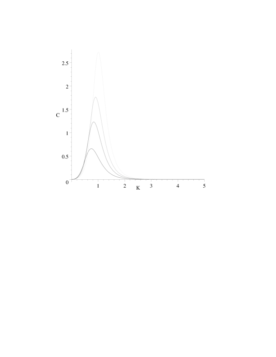
Figure 21: Specific heat (with $k_{B}\equiv 1$) for the Potts ferromagnet on the infinite-length, width $L_{y}=2$ strip of the $sq_{d}$ lattice, as a function of $K=J/(k_{B}T)$. Going from bottom to top in order of the heights of the maxima, the curves are for $q=2,3,4,6$.

The high-temperature expansion of $U$ is

$$U=-\frac{5J}{2q}\biggl{[}1+\frac{(q-1)}{q}K+O(K^{2})\biggr{]}\ .$$ (3.5.1)

For the specific heat we have

$$C=\frac{5k_{B}(q-1)K^{2}}{2q^{2}}\biggl{[}1+\frac{(5q+14)}{5q}K+O(K^{2})\biggr{]}\ .$$ (3.5.2)

The low-temperature expansions ($K\to\infty$) are

$$U=J\Biggl{[}-\frac{5}{2}+2(q-1)e^{-4K}\biggl{[}1+5e^{-K}+7(q-2)e^{-2K}+O(e^{-3K})\biggr{]}\Biggr{]}\quad{\rm as}\quad K\to\infty$$ (3.5.3)

and

$$C=8k_{B}K^{2}(q-1)e^{-4K}\biggl{[}1+\frac{25}{4}e^{-K}+\frac{49}{4}(q-2)e^{-3K}+O(e^{-4K})\biggr{]}\quad{\rm as}\quad K\to\infty$$ (3.5.4)

Comparing with our corresponding calculations for the ($L_{x}\to\infty$ limits of the) strips of the square and triangular lattices with the same $L_{y}=2$ width, we can remark on some common features. In all of these cases, the high-temperature expansions have the leading forms

$$U=-\frac{\Delta J}{2q}\biggl{[}1+\frac{(q-1)}{q}K+O(K^{2})\biggr{]}$$ (3.5.5)

where we recall that the coordination number is $\Delta=3,4$ and 5 for these infinite-length strips of the square, triangular, and $sq_{d}$ lattices with width 2. (In the infinite-length limit, the longitudinal boundary conditions do not affect the coordination number.) Further,

$$C=\frac{\Delta k_{B}(q-1)K^{2}}{2q^{2}}\biggl{[}1+O(K)\biggr{]}\ .$$ (3.5.6)

For the low-temperature expansions for these strips,

$$U=J\Biggl{[}-\frac{\Delta}{2}+O((q-1)e^{-(\Delta-1)K})\Biggr{]}\quad{\rm as}\quad K\to\infty$$ (3.5.7)

and

$$C\propto k_{B}K^{2}(q-1)e^{-(\Delta-1)K}\biggl{[}1+O(e^{-K})\biggr{]}\quad{\rm as}\quad K\to\infty\ .$$ (3.5.8)

In general, the ratio $\rho$ of the largest subdominant to the dominant $\lambda_{j}$’s determines the asymptotic decay of the connected spin-spin correlation function and hence the correlation length

$$\xi=-\frac{1}{\ln\rho}$$ (3.5.9)

Since $\lambda_{L,4}$ and $\lambda_{L,2}$ are the dominant and leading subdominant $\lambda_{j}$’s, respectively, we have

$$\rho_{FM}=\frac{\lambda_{L,2}}{\lambda_{L,4}}$$ (3.5.10)

and hence for the ferromagnetic zero-temperature critical point we find that the correlation length diverges, as $T\to 0$, as

$$\xi_{FM}\sim q^{-1}e^{4K}\quad{\rm as}\quad K\to\infty$$ (3.5.11)

Comparing with the divergences in the correlation length at the ferromagnetic $T=0$ critical point that we have calculated for the infinite-length limits of the square and triangular strips with the same $L_{y}=2$ width [15, 16], we see that all of these can be fit by the formula

$$\xi_{FM}\sim q^{-1}e^{(\Delta-1)K}\quad{\rm as}\quad K\to\infty\ .$$ (3.5.12)

3.5.2 Antiferromagnetic Case

In this section we first restrict to the real range $q\geq 4$ and the additional integer values $q=2$ (Ising case) and $q=3$ where the Potts antiferromagnet exhibits physically acceptable behavior and then consider the remaining interval $0<q<4$, $q\neq 2,3$, where it exhibits unphysical properties. For $q\geq 4$, the free energy is given for all temperatures by (2.16), as in the ferromagnetic case but with $J$ negative, and is the same independent of the different longitudinal boundary conditions, as is necessary for there to exist a thermodynamic limit.

We show plots of the specific heat, for several values of $q$, for the Potts antiferromagnet on the (infinite-length limit of the) $L_{y}=2$ strip of the $sq_{d}$ lattice in Fig 22. In contrast to the ferromagnetic case, where the positions of the maxima of $C$ in the variable $K$ increase monotonically as functions of $q$, the positions of the maxima of $C$ in the antiferromagnetic do not have a monotonic dependence on $q$; they occur at $K=-0.82$ for $q=2$, $K=-0.42$ for $q=3$ and $K=-0.75$ for $q=4$, after which the values of the maxima occur at smaller values of $-K$ with increasing integral $q$, e.g., $K=-0.47$ for $q=5$ and $K=-0.34$ for $q=6$). Recall that the antiferromagnetic Potts model with $q=2$ and $q=3$ involves frustration, and one can observe a rather different behavior in the specific heat for these values of $q$ as contrasted with $q\geq 4$ in the plot.

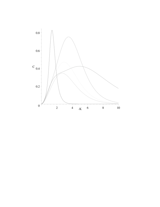
Figure 22: Specific heat (with $k_{B}\equiv 1$) for the Potts antiferromagnet on the infinite-length, width $L_{y}=2$ strip of the $sq_{d}$ lattice, as a function of $-K=-J/(k_{B}T)$. Going downward in order of the heights of the maxima, the curves are for $q=2,4,5,3,6$.

The high-temperature expansions of $U$ and $C$ are given by (3.5.1) and (3.5.2); more generally, these expansions also apply in the range $0<q<4$. As discussed above, the Ising case $q=2$ is one of the cases where one must take account of noncommutativity in the definition of the free energy and hence of thermodynamic quantities. If one sets $q=2$ first and then takes $n\to\infty$, then $f=f_{nq}=(1/2)\ln\lambda_{L,4}(q=2)$ where $\lambda_{L,4}(q=2)$ was given in eq. (3.2.16), and the low-temperature expansions are

$$U(q=2)=-\frac{J}{2}\biggl{[}1+12e^{3K}+36e^{4K}+80e^{5K}+O(e^{6K})\biggr{]}\quad{\rm as}\quad K\to-\infty$$ (3.5.13)

and

$$C(q=2)=18k_{B}K^{2}e^{3K}\biggl{[}1+4e^{K}+\frac{100}{9}e^{2K}+\frac{72}{9}e^{3K}+O(e^{4K})\biggr{]}\quad{\rm as}\quad K\to-\infty\ .$$ (3.5.14)

For $q=3$, if one sets $q=3$ first and then takes $n\to\infty$, then $f=f_{nq}=(1/2)\ln\lambda_{L,4}(q=3)$, and the low-temperature expansions are

$$U(q=3)=-\frac{J}{4}\biggl{[}1+\frac{3\sqrt{2}}{2}e^{K/2}-4e^{K}+\frac{57\sqrt{2}}{8}e^{3K/2}+O(e^{2K})\biggr{]}\quad{\rm as}\quad K\to-\infty$$ (3.5.15)

and

$$C(q=3)=\frac{3\sqrt{2}}{16}k_{B}K^{2}e^{K/2}\biggl{[}1-\frac{8\sqrt{2}}{3}e^{K/2}+\frac{57}{4}e^{K}-16\sqrt{2}e^{3K/2}+O(e^{2K})\biggr{]}\quad{\rm as}\quad K\to-\infty\ .$$ (3.5.16)

For the range $q\geq 4$, the low-temperature expansions are given by

$$U=\frac{(-J)e^{K}}{2(q-3)^{2}}\biggl{[}(5q-13)-\frac{29q^{3}-190q^{2}+405q-276}{(q-3)^{2}(q-2)}e^{K}+O(e^{2K})\biggr{]}\quad{\rm as}\quad K\to-\infty$$ (3.5.17)

and

$$C=\frac{k_{B}K^{2}e^{K}}{2(q-3)^{2}}\biggl{[}(5q-13)-\frac{2(29q^{3}-190q^{2}+405q-276)}{(q-3)^{2}(q-2)}e^{K}+O(e^{2K})\biggr{]}\quad{\rm as}\quad K\to-\infty\ .$$ (3.5.18)

Note that for the antiferromagnetic case, $U(T=0)=0$ for $q\geq 4$, but $U(T=0)=-J/2=+|J|/2$ for $q=2$ and $U(T=0)=-J/4=+|J|/4$ for $q=3$. The vanishing value of $U$ at $T=0$ for $q\geq 4$ means that the Potts model can achieve its preferred ground state for this range of $q$, while the nonzero value of $U(T=0)$ for the Ising and $q=3$ antiferromagnet is a consequence of the frustration that is present in this case. Note that the apparent divergences that occur as $q\to 2$ and $q\to 3$ in eqs. (3.5.17) and (3.5.18) are not actually reached here since these expressions apply only in the region $q\geq 4$ (the discrete integral cases $q=2$ and $q=3$ were dealt with above).

For the zero-temperature critical points in the $q=2$ and $q=4$ Potts antiferromagnet,

$$\rho_{AFM,q=2,4}=\frac{\lambda_{L,2}}{\lambda_{L,4}}$$ (3.5.19)

Using the respective expansions (3.2.24)-(3.2.25) and (3.2.27)-(3.2.30), we find that the correlation lengths defined as in (3.5.9) diverges, as $T\to 0$, as

$$\xi_{AFM,q=2}\sim e^{-3K}\ ,\quad{\rm as}\quad K\to-\infty$$ (3.5.20)

and

$$\xi_{AFM,q=4}\sim e^{-K}\ ,\quad{\rm as}\quad K\to-\infty\ .$$ (3.5.21)

Next, we consider the range of real $0<q<4$ aside from the integral case $q=2,3$. The first pathology is that the Potts antiferromagnet on the infinite-length limit of the cyclic $L_{y}=2$ $sq_{d}$ strip has a phase transition at a finite temperature, call it $T_{p,L}$, while, in contrast, if one uses free boundary conditions, then either (i) there is no phase transition at any finite temperature, for $3<q<4$ or $1<q<2$, or (ii) there is a phase transition at a finite temperature $T_{p,S}$ for $2<q<3$ or $0<q<1$, but $T_{p,L}\neq T_{p,S}$, so that there is no well-defined thermodynamic limit for the Potts antiferromagnet with non-integral $q$ in the interval $0<q<4$. The Ising case $q=2$ and $q=3$ case have been dealt with in the preceding subsection. Concerning the value $q=1$, as discussed earlier, one encounters noncommutativity in defining the free energy. If one takes $q=1$ to start with and then $n\to\infty$, the thermodynamic limit does exist, independent of boundary conditions, and $f=f_{nq}=2.5K$, $U=-2.5J=2.5|J|$, and $C=0$. If one starts with $q\neq 1$, takes $n\to\infty$, calculates $f_{qn}$, and then takes $q\to 1$, the thermodynamic limit does not exist since the result differs depending on whether one uses free longitudinal boundary conditions or cyclic longitudinal boundary conditions. In the high-temperature phase, $f_{qn}=(1/2)\ln\lambda_{L,4}$, independent of longitudinal boundary conditions, but in the low-temperature phase, the expression for $f_{qn}$ is different for the open and cyclic strips. There are also other unphysical properties, such as a negative specific heat and a negative partition function for certain ranges of temperature.

Acknowledgment: The research of R. S. was supported in part at Stony Brook by the U. S. NSF grant PHY-97-22101 and at Brookhaven by the U.S. DOE contract DE-AC02-98CH10886.

4 Appendix

4.1 General

The Potts model partition function $Z(G,q,v)$ is related to the Tutte polynomial $T(G,x,y)$ as follows. The graph $G$ has vertex set $V$ and edge set $E$, denoted $G=(V,E)$. A spanning subgraph $G^{\prime}$ is defined as a subgraph that has the same vertex set and a subset of the edge set: $G^{\prime}=(V,E^{\prime})$ with $E^{\prime}\subseteq E$. The Tutte polynomial of $G$, $T(G,x,y)$, is then given by [6]-[8]

$$T(G,x,y)=\sum_{G^{\prime}\subseteq G}(x-1)^{k(G^{\prime})-k(G)}(y-1)^{c(G^{\prime})}$$ (4.1.1)

where $k(G^{\prime})$, $e(G^{\prime})$, and $n(G^{\prime})=n(G)$ denote the number of components, edges, and vertices of $G^{\prime}$, and

$$c(G^{\prime})=e(G^{\prime})+k(G^{\prime})-n(G^{\prime})$$ (4.1.2)

is the number of independent circuits in $G^{\prime}$ (sometimes called the co-rank of $G^{\prime}$). Note that the first factor can also be written as $(x-1)^{r(G)-r(G^{\prime})}$, where

$$r(G)=n(G)-k(G)$$ (4.1.3)

is called the rank of $G$. The graphs $G$ that we consider here are connected, so that $k(G)=1$. Now let

$$x=1+\frac{q}{v}$$ (4.1.4)

and

$$y=a=v+1$$ (4.1.5)

so that

$$q=(x-1)(y-1)\ .$$ (4.1.6)

Then

$$Z(G,q,v)=(x-1)^{k(G)}(y-1)^{n(G)}T(G,x,y)\ .$$ (4.1.7)

Note that the chromatic polynomial is a special case of the Tutte polynomial:

$$P(G,q)=q^{k(G)}(-1)^{k(G)+n(G)}T(G,x=1-q,y=0)$$ (4.1.8)

(recall eq. (1.9)).

Corresponding to the form (1.25) we find that the Tutte polynomial for recursively defined graphs comprised of $m$ repetitions of some subgraph has the form

$$T(G_{m},x,y)=\sum_{j=1}^{N_{\lambda}}c_{T,G,j}(\lambda_{T,G,j})^{m}$$ (4.1.9)

4.2 $sq_{d}$ Strip with Free Longitudinal Boundary Conditions

The generating function representation for the Tutte polynomial for the open strip of the $sq_{d}$ lattice comprised of $m+1$ squares with edges joining the lower-left to upper-right vertices and the upper-left to lower-right vertices of each square, denoted $S_{m}$, is

$$\Gamma_{T}(S_{m},x,y;z)=\sum_{m=0}^{\infty}T(S_{m},x,y)z^{m}\ .$$ (4.2.1)

We have

$$\Gamma_{T}(S,x,y;z)=\frac{{\cal N}_{T}(S,x,y;z)}{{\cal D}_{T}(S,x,y;z)}$$ (4.2.2)

where

$${\cal N}_{T}(S,x,y;z)=A_{T,S,0}+A_{T,S,1}z$$ (4.2.3)

with

$$A_{T,S,0}=2x+4xy+3x^{2}+2y+3y^{2}+y^{3}+x^{3}$$ (4.2.4)

$$A_{T,S,1}=xy(y+y^{2}+x-2xy^{2}+xy+x^{2}-2yx^{2}-x^{2}y^{2})$$ (4.2.5)

and

$${\cal D}_{T}(S,x,y;z)=\prod_{j=1}^{2}(1-\lambda_{T,S,j}z)$$ (4.2.6)

with

$$\lambda_{T,S,(1,2)}=\frac{1}{2}\biggl{[}x(x+3)+y(y^{2}+2y+3)+2\pm\sqrt{R_{T}}\ \biggr{]}$$ (4.2.7)

where

$$R_{T} = 4+12x+12y+22xy+13x^{2}+21y^{2}+6x^{3}+20y^{3}+16xy^{2}$$ (4.2.10)

$$+10x^{2}y+x^{4}+10y^{4}-4x^{2}y^{2}-2y^{3}x+4y^{5}-2x^{2}y^{3}+y^{6}\ .$$

The corresponding closed-form expression is given by the general formula from [22], as applied to Tutte, rather than chromatic, polynomials, namely

$$T(S_{m},x,y)=\biggl{[}\frac{A_{T,S,0}\lambda_{T,S,1}+A_{T,S,1}}{\lambda_{T,S,1}-\lambda_{T,S,2}}\biggr{]}(\lambda_{T,S,1})^{m}+\biggl{[}\frac{A_{T,S,0}\lambda_{T,S,2}+A_{T,S,1}}{\lambda_{T,S,2}-\lambda_{T,S,1}}\biggr{]}(\lambda_{T,S,2})^{m}\ .$$ (4.2.11)

It is easily checked that this is a symmetric function of the $\lambda_{S,j}$, $j=1,2$.

4.3 Cyclic and Möbius Strips

We write the Tutte polynomials for the cyclic and Möbius strips of the $sq_{d}$ lattice with width $L_{y}=2$ as

$$T(L_{m},x,y)=\sum_{j=1}^{5}c_{T,L,j}(\lambda_{T,L,j})^{m}$$ (4.3.1)

where it is convenient to extract a common factor from the coefficients:

$$c_{T,L,j}\equiv\frac{\bar{c}_{T,L,j}}{x-1}\ .$$ (4.3.2)

Of course, although the individual terms contributing to the Tutte polynomial are thus rational functions of $x$ rather than polynomials in $x$, the full Tutte polynomial is a polynomial in both $x$ and $y$. We have

$$\lambda_{T,L,1}=2$$ (4.3.3)

and, with

$$T_{T,23}=y^{3}+2y^{2}+3y+2x+4$$ (4.3.4)

$$R_{T,23}=16+16x+32y+12xy+33y^{2}-4xy^{3}+10y^{4}+4x^{2}+20y^{3}+4y^{5}+y^{6}$$ (4.3.5)

the results

$$\lambda_{T,L,(2,3)}=\frac{1}{2}\biggl{[}T_{T,23}\pm\sqrt{R_{T,23}}\ \biggr{]}$$ (4.3.6)

and

$$\lambda_{T,L,(4,5)}=\lambda_{T,S,(1,2)}$$ (4.3.7)

The coefficients are

$$\bar{c}_{T,L,1}=\frac{1}{2}(x-1)(y-1)(xy-x-y-2)$$ (4.3.8)

$$\bar{c}_{T,L,2}=\bar{c}_{T,L,3}=xy-x-y$$ (4.3.9)

$$\bar{c}_{T,L,4}=\bar{c}_{T,L,5}=1\ .$$ (4.3.10)

These are symmetric under interchange of $x\leftrightarrow y$, which is a consequence of the fact that the $c_{L,j}$ are functions only of $q$.

4.4 Special Values of Tutte Polynomials for Strips of the $sq_{d}$ Lattice

For a given graph $G=(V,E)$, at certain special values of the arguments $x$ and $y$, the Tutte polynomial $T(G,x,y)$ yields quantities of basic graph-theoretic interest [8]-[13], [39]. We recall some definitions: a spanning subgraph $G^{\prime}=(V,E^{\prime})$ of $G$ is a graph with the same vertex set $V$ and a subset of the edge set, $E^{\prime}\subseteq E$. Furthermore, a tree is a graph with no cycles, and a forest is a graph containing one or more trees. Then the number of spanning trees of $G$, $N_{ST}(G)$, is

$$N_{ST}(G)=T(G,1,1)\ ,$$ (4.4.1)

the number of spanning forests of $G$, $N_{SF}(G)$, is

$$N_{SF}(G)=T(G,2,1)\ ,$$ (4.4.2)

the number of connected spanning subgraphs of $G$, $N_{CSSG}(G)$, is

$$N_{CSSG}(G)=T(G,1,2)\ ,$$ (4.4.3)

and the number of spanning subgraphs of $G$, $N_{SSG}(G)$, is

$$N_{SSG}(G)=T(G,2,2)\ .$$ (4.4.4)

From our calculations of Tutte polynomials, we find that

$$N_{ST}(S_{m})=2^{2(m+2)}\cdot 3^{m}$$ (4.4.5)

$$N_{SF}(S_{m})=(19+11\sqrt{3}\ )(9+5\sqrt{3}\ )^{m}+(19-11\sqrt{3}\ )(9-5\sqrt{3}\ )^{m}$$ (4.4.6)

$$N_{CSSG}(S_{m})=\Bigl{(}19+\frac{65\sqrt{46}}{23}\ \Bigr{)}[2(7+\sqrt{46}\ )]^{m}+\Bigl{(}19-\frac{65\sqrt{46}}{23}\ \Bigr{)}[2(7-\sqrt{46}\ )]^{m}$$ (4.4.7)

$$N_{SSG}(S_{m})=2^{5m+6}\ .$$ (4.4.8)

For the cyclic $L_{y}=2$ strip of the $sq_{d}$ lattice, $L_{m}$, we first note that for $m\geq 3$, $L_{m}$ is a (proper) graph, but for $m=1$ and $m=2$, $L_{m}$ is not a proper graph, but instead, is a multigraph, with multiple edges (and, for $m=1$, loops). The following formulas apply for all $m\geq 1$:

$$N_{ST}(L_{m})=2^{2(m-1)}\cdot 3^{m}m$$ (4.4.9)

$$N_{SF}(L_{m})=\biggl{[}\Bigl{(}9+5\sqrt{3}\ \Bigr{)}^{m}+\Bigl{(}9-5\sqrt{3}\ \Bigr{)}^{m}\biggl{]}-\biggl{[}\Bigl{(}7+3\sqrt{5}\ \Bigr{)}^{m}+\Bigl{(}7-3\sqrt{5}\ \Bigr{)}^{m}\biggl{]}$$ (4.4.10)

$$N_{CSSG}(L_{m})=-3\cdot 2^{m-1}+\biggl{[}2\Bigl{(}7+\sqrt{46}\ \Bigr{)}\biggr{]}^{m}+\biggl{[}2\Bigl{(}7-\sqrt{46}\ \Bigr{)}\biggr{]}^{m}+$$ (4.4.11)

(4.4.12)

$$\frac{m}{2}\Biggl{[}\Bigl{(}3+\frac{7\sqrt{46}}{23}\ \Bigr{)}\biggl{[}2\Bigl{(}7+\sqrt{46}\ \Bigr{)}\biggr{]}^{m-1}+\Bigl{(}3-\frac{7\sqrt{46}}{23}\ \Bigr{)}\biggl{[}2\Bigl{(}7-\sqrt{46}\ \Bigr{)}\biggr{]}^{m-1}\Biggr{]}$$ (4.4.13)

$$N_{SSG}(L_{m})=2^{5m}\ .$$ (4.4.14)

This result, eq. (4.4.14), is a special case of a more general elementary theorem, namely

$$N_{SSG}(G)=2^{e(G)}$$ (4.4.15)

This is proved by noting that a spanning subgraph $G^{\prime}\subseteq G$ consists of the same vertex set $V$ as $G$ and a subset of the edge set $E$ of $G$. One can enumerate all such spanning subgraphs as follows: for each edge in $E$, one has the option of including or excluding it, keeping the other edges fixed. This is a twofold choice for each edge, and the result (4.4.15) therefore holds. This general result subsumes the previous specific relations $N_{SSG}=2^{3m}$ and $N_{SSG}=2^{4m}$ for the cyclic strips of length $L_{x}=m$ and width $L_{y}=2$ of the square and triangular lattices. We recall that the number of edges is given by $e(G)=$ (i) $3m$, (ii) $4m$, and (iii) $5m$ for the $L_{x}=m$, $L_{y}=2$ strips of the (i) square (ii) triangular, (iii) $sq_{d}$ strips, respectively, while the number of vertices is given by $n=v(G)=2m$ for all of these strips. Let us denote $r_{e}=e(G)/n(G)$, whence $r_{e}(G)=$ (i) 3/2, (ii) 2, (iii) $5/2$ and $N_{SSG}(L_{G,m})=2^{r_{e}(G)n}$ for these strips.

Since $T(G_{m},x,y)$ grows exponentially as $m\to\infty$ for the families $G_{m}=S_{m}$ and $L_{m}$ for $(x,y)=(1,1)$, (2,1), (1,2), and (2,2), one defines the corresponding constants

$$z_{set}(\{G\})=\lim_{n(G)\to\infty}n(G)^{-1}\ln N_{set}(G)\ ,\quad set=ST,\ SF,\ CSSG,\ SSG$$ (4.4.16)

where, as above, the symbol $\{G\}$ denotes the limit of the graph family $G$ as $n(G)\to\infty$ (and the $z$ here should not be confused with the auxiliary expansion variable in the generating function (4.2.1) or the Potts partition function $Z(G,q,v)$.) General inequalities for these were given in [15].

Our results yield

$$z_{ST}(\{G\})=\ln 2+\frac{1}{2}\ln 3\simeq 1.242453..\quad{\rm for}\quad G=S,L$$ (4.4.17)

$$z_{SF}(\{G\})=\frac{1}{2}\ln(9+5\sqrt{3}\ )\simeq 1.435658\quad{\rm for}\quad G=S,L$$ (4.4.18)

$$z_{CSSG}(\{G\})=\frac{1}{2}\ln[2(7+\sqrt{46}\ )]\simeq 1.658267\quad{\rm for}\quad G=S,L$$ (4.4.19)

and

$$z_{SSG}(\{G\})=\frac{5}{2}\ln 2\simeq 1.732868\quad{\rm for}\quad G=S,L$$ (4.4.20)

In Table I we summarize the results for $z_{s}(\{G\})$ for the infinite-length limit of the width $L_{y}=2$ strips of the square, triangular, and $sq_{d}$ strips (which are independent of the longitudinal boundary conditions). In this table we include a comparison of the exact values of $z_{ST}$ that we have calculated with the upper bound (u.b.) for a $k$-regular graph [38]

$$z_{ST}<z_{ST,u.b.}\ ,\quad z_{ST,u.b.}=\ln\Biggl{(}\frac{(k-1)^{k-1}}{[k(k-2)]^{(k/2)-1}}\Biggr{)}$$ (4.4.21)

The cyclic $L_{y}=2$ strips of the square, triangular, and $sq_{d}$ lattices are $k$-regular, with $k=3,4,5$, respectively. One thus has

$$z_{ST,u.b.}(sq(L_{y}=2))=\ln(4/\sqrt{3})$$ (4.4.22)

$$z_{ST,u.b.}(tri(L_{y}=2))=3\ln(3/2)$$ (4.4.23)

$$z_{ST,u.b.}(sq_{d}(L_{y}=2))=8\ln 2-\frac{3}{2}\ln 15$$ (4.4.24)

For this table we define

$$r_{ST}(\{G\})=\frac{z_{ST}(\{G\})}{z_{ST,u.b.}(\{G\})}\ .$$ (4.4.25)

As is evident from the table, $z_{ST}(\{G\})$, $z_{SF}(\{G\})$, and $z_{CSSG}(\{G\})$ increase as one goes from the $L_{y}=2$ strip of the square strip to that of the triangular, and $sq_{d}$ strip, as the degree increases from 3 to 4 to 5. This also follows from (4.4.15) for $z_{SSG}$. A similar dependence on degree (coordination number) was found for $z_{ST}$ in [39, 40].

Table 1: $z_{s}(\{G\})$ for the $L_{x}\to\infty$ limit of the width $L_{y}=2$ strips of the (i) square lattice, (ii) triangular lattice (constructed by starting with a square strip and adding edges joining the lower left to upper right vertex of each square, and (iii) $sq_{d}$ lattice, i.e., square lattice with next-nearest-neighbor couplings.

$z_{s}(\{G\})$	$\{G\}=sq$	$\{G\}=tri$	$\{G\}=sq_{d}$
$z_{ST}(\{G\})$	$(1/2)\ln(2+\sqrt{3}\ )$	$(1/2)\ln[(7+3\sqrt{5}\ )/2]$	$\ln(2\sqrt{3}\ )$
	$=0.658479$	$=0.962424$	$=1.242453$
$r_{ST}(\{G\})$	0.7867	0.7912	0.8377
$z_{SF}(\{G\})$	$(1/2)\ln[2(2+\sqrt{3}\ )]$	$(1/2)\ln[2(3+2\sqrt{2}\ )]$	$(1/2)\ln(9+5\sqrt{3}\ )$
	$=1.005053$	$=1.227947$	$=1.435658$
$z_{CSSG}(\{G\})$	$(1/2)\ln[(5+\sqrt{17}\ )/2]$	$(1/2)\ln[2(3+2\sqrt{2}\ )]$	$(1/2)\ln[2(7+\sqrt{46}\ )]$
	$=0.758832$	$=1.227947$	$=1.658267$
$z_{SSG}(\{G\})$	$(3/2)\ln 2$	$2\ln 2$	$(5/2)\ln 2$
	$1.039721$	$=1.386294$	$=1.732868$

References

• [1] R. B. Potts, Proc. Camb. Phil. Soc. 48, 106 (1952).
• [2] F. Y. Wu, Rev. Mod. Phys. 54, 235 (1982).
• [3] G. D. Birkhoff, Ann. of Math. 14, 42 (1912).
• [4] H. Whitney, Ann. of Math. 33, 688 (1932).
• [5] P. W. Kasteleyn and C. M. Fortuin, J. Phys. Soc. Jpn. (Suppl.) 26, 11 (1969); C. M. Fortuin and P. W. Kasteleyn, Physica 57, 536 (1972).
• [6] W. T. Tutte, Can. J. Math. 6, 80 (1954).
• [7] W. T. Tutte, J. Combin. Theory 2, 301 (1967).
• [8] W. T. Tutte, J. Combin. Theory 2, 301 (1967).
• [9] W. T. Tutte, β€œChromials”, in Lecture Notes in Math. v. 411, p. 243 (1974).
• [10] W. T. Tutte, Graph Theory, vol. 21 of Encyclopedia of Mathematics and Applications (Addison-Wesley, Menlo Park, 1984).
• [11] N. L. Biggs, Algebraic Graph Theory (2nd ed., Cambridge Univ. Press, Cambridge, 1993).
• [12] D. J. A. Welsh, Complexity: Knots, Colourings, and Counting, London Math. Soc. Lect. Note Ser. 186 (Cambridge University Press, Cambridge, 1993).
• [13] B. BollobΓ‘s, Modern Graph Theory (Springer, New York, 1998).
• [14] R. Shrock, in Proceedings of the 1999 British Combinatorial Conference, BCC99, Discrete Math., in press.
• [15] R. Shrock, Physica A 283, 388 (2000).
• [16] S.-C. Chang and R. Shrock, Physica A, in press (cond-mat/0004181).
• [17] R. Shrock and S.-H. Tsai, Phys. Rev. E55, 5184 (1997).
• [18] H. Kluepfel and R. Shrock, to appear; H. Kluepfel, Stony Brook thesis (July, 1999).
• [19] R. Shrock and S.-H. Tsai, Phys. Rev. E56, 2733 (1997).
• [20] S.-C. Chang and R. Shrock, Phys. Rev. E, in press (cond-mat/0005236).
• [21] M. Roček, R. Shrock, and S.-H. Tsai, Physica A252, 505 (1998).
• [22] R. Shrock and S.-H. Tsai, Physica A259, 315 (1998).
• [23] R. C. Read, J. Combin. Theory 4, 52 (1968).
• [24] R. C. Read and W. T. Tutte, β€œChromatic Polynomials”, in Selected Topics in Graph Theory, 3, eds. L. W. Beineke and R. J. Wilson (Academic Press, New York, 1988.).
• [25] N. L. Biggs, R. M. Damerell, and D. A. Sands, J. Combin. Theory B 12, 123 (1972).
• [26] S. Beraha, J. Kahane, and N. Weiss, J. Combin. Theory B 28, 52 (1980).
• [27] R. C. Read, in Proc. 5th Caribbean Conf. on Combin. and Computing (1988).
• [28] R. C. Read and G. F. Royle, in Graph Theory, Combinatorics, and Applications (Wiley, NY, 1991), vol. 2, p. 1009.
• [29] R. Shrock and S.-H. Tsai, Phys. Rev. E55, 5165 (1997).
• [30] M. E. Fisher, Lectures in Theoretical Physics (Univ. of Colorado Press, Boulder, 1965), vol. 7C, p. 1.
• [31] S.-C. Chang and R. Shrock, Physica A, in press (cond-mat/0004161).
• [32] V. Matveev and R. Shrock, J. Phys. A 28, 1557 (1995).
• [33] R. Shrock, Phys. Lett. A261, 57 (1999).
• [34] J. V. Uspensky, Theory of Equations (McGraw-Hill, NY 1948), 264.
• [35] S.-C. Chang and R. Shrock, cond-mat/0005232.
• [36] R. J. Walker, Algebraic Curves (Princeton Univ. Press, Princeton, 1950); R. Hartshorne, Algebraic Geometry (Springer, New York, 1977).
• [37] M. E. Fisher, Lectures in Theoretical Physics (Univ. of Colorado Press, Boulder, 1965), vol. 7C, p. 1.
• [38] B. McKay, J. Combinatorics 4, 149 (1983); F. Chung and S.-T. Yau, www.combinatorics.org R12, 6 (1999).
• [39] F. Y. Wu, J. Phys. A 10, L113 (1977).
• [40] W.-J. Tzeng and F. Y. Wu, cond-mat/0001408; R. Shrock, F. Y. Wu, J. Phys. A 33 3881 (2000).